Minimum bias multiple taper spectral estimation

Minimum bias multiple taper spectral

estimation

∗

Kurt S. Riedel and Alexander Sidorenko

Courant Institute of Mathematical Sciences, New York University

New York, New York 10012-1185

EDICS: SP 3.1.1

Abstract

Two families of orthonormal tapers are proposed for multitaper spectral analysis: minimum bias tapers, and sinusoidal tapers {v(k)}, where v(nk) =

q

2

N+1sin

πkn

N+1, and N is the number of points. The

re-sulting sinusoidal multitaper spectral estimate is ˆS(f) = _2K(N1₊₁₎PK

j=1|y(f+

j

2N+2)−y(f−

j

2N+2)|

2_{, wherey(f) is the Fourier transform of the}

sta-tionary time series,S(f) is the spectral density, andK is the number of tapers. For fixedj, the sinusoidal tapers converge to the minimum bias tapers like 1/N. Since the sinusoidal tapers have analytic ex-pressions, no numerical eigenvalue decomposition is necessary. Both the minimum bias and sinusoidal tapers have no additional parame-ter for the spectral bandwidth. The bandwidth of the jth taper is simply _N1 centered about the frequencies _2N±₊₂j . Thus the bandwidth of the multitaper spectral estimate can be adjusted locally by simply adding or deleting tapers. The band limited spectral concentration,

Rw

−w|V(f)|2df, of both the minimum bias and sinusoidal tapers is very

close to the optimal concentration achieved by the Slepian tapers. In contrast, the Slepian tapers can have the local bias,R1/2

−1/2f

2_|V(f)|2_df,

much larger than of the minimum bias tapers and the sinusoidal ta-pers.

∗_{The authors thank D. J. Thomson and the referees for useful comments. Research}

funded by the U.S. Department of Energy.

1

Introduction

We consider a stationary time series, {xn, n = 1. . . N} with a spectral

den-sity, S(f). A common estimator of the spectral density is to smooth the

square of the discrete Fourier transform (DFT) locally: ˆ S(f) = 1 (2L+ 1)N L X j=−L |y(f + j N)| 2_{, (1)}

where y(f) is the Fourier transform (FT) of the stationary time series:

y(f) ≡ PN

n=1xne−i2πnf . Since (1) is quadratic in the FT, y(f), it is

natural to consider a more general class of quadratic spectral estimators. We examine quadratic estimators where the underlying self-adjoint matrix has rank K, where K is prescribed. Using the eigenvector representation, the

resulting quadratic spectral estimator can be recast as a weighted sum of K

orthonormal rank one spectral estimators. This class of spectral estimators was originally proposed by Thomson [19] under the name of multiple taper spectral analysis (MTSA). We refer the reader to [3, 8, 11, 12, 16, 18, 19] for excellent expositions and generalizations of Thomson’s theory.

In MTSA, a rankK quadratic spectral estimate is constructed by

choos-ing an orthonormal family of tapers/spectral windows and then averagchoos-ing

the K estimates of the spectral density. In practice, only the Slepian tapers

(also known as discrete prolate spheroidal sequences [17]) are routinely used for MTSA.

In the present paper, we propose and analyze two new orthonormal fam-ilies of tapers: minimum bias (MB) tapers and sinusoidal tapers. The MB

tapers minimize the local frequency bias, R

f2_|V(f)|2_{df, subject to}

orthonor-mality constraints, whereV(f) is the DFT of the taper. For continuous time,

the MB tapers have simple analytic expressions. The first taper in the fam-ily is Papoulis’ optimal taper [9]. For discrete time, the MB tapers satisfy a selfadjoint eigenvalue problem and may be computed numerically.

In the case of discrete time, we define the kth sinusoidal taper, v(k)_{, as}

v(k)

n =

q ₂

N+1sin

πkn

N+1, where N is the sequence length. The sinusoidal tapers

are an orthonormal family that converge to the MB tapers with rate 1/N as

N → ∞. These results are given in Section 3. Section 4 compares the local

bias, R1/2

−1/2f

2_|V(f)|2_{df, and the spectral concentration,} Rw

−w|V(f)|2df, of the

In Section 5, we show that the quadratic spectral estimator which mini-mizes the expected square local error is weighted multitaper estimate using the MB tapers. A local error analysis is given and the optimal number of tapers is determined. At frequencies where the spectral density is chang-ing rapidly, fewer tapers should be used. In Section 6, we show that kernel smoother spectral estimates [4, 10] are multitaper estimates and we show that smoothing the logarithm of the multitaper estimate significantly re-duces the variance in comparison with smoothing athe logarithm of a single taper estimate. We also describe our data adaptive method for estimating the spectrum. In Section 7, we apply our spectral estimation techniques to real data and show that our tapers outperform the Slepian tapers whenever a variable bandwidth is needed. In the Appendix, we show that the leading principal components of kernel smoother spectral estimates resemble the MB tapers.

2

Quadratic Estimators of the Power

Spec-trum

Let N discrete measurements, x1, x2, . . . , xN, be given as a realization of

a stationary stochastic process. We normalize the time interval between measurements to unity. The Cramer representation of a discrete stationary stochastic process [4, 12] is

x(t) =

Z 1/2

−1/2

e2πinfdZ(f),

wheredZ has independent spectral increments: E[dZ(f)dZ(g)] = S(f)δ(f−

g)df dg. We assume that the spectral density, S(f), is twice continuously differentiable.

The spectral inverse problem is to estimate the spectral density, S(f),

given {xn}. As shown in [3, 8], every quadratic, modulation-invariant power

spectrum estimator has the form:

b S(f) = N X n,m=1 qnme2πi(m−n)fxnxm , (2)

where Q = [qnm] is a symmetric matrix of order N and does not depend on

frequency. Consider the eigenvector decomposition: Q =PK

k=1µkv(k)

where K is the rank of Q, and v(1)_,v(2)_{, . . . ,v}(K) _{is an orthogonal system}

of eigenvectors. The multitaper representation of the quadratic spectral es-timator is b S(f) = K X k=1 µk N X n=1 v_n(k)xne−2πinf 2 . (3)

In the case K = 1, estimator (3) turns out atapered periodogram estimator:

b Sv(f) = N X n=1 vnxne−2πinf 2 , (4)

with a taper v= (v1, v2, . . . , vN)T. If the tapering is uniform (i.e. v1 =v2 =

. . .=vN = √1_N), we name (4) the periodogram estimator. The estimator (3)

is a linear combination of K orthogonal tapered periodogram estimators. In

MTSA, K is normally chosen to be much less than N. The multiple taper

spectral estimate can be thought of as a low rank, “principal components” approximation of a general quadratic estimator. Multiple taper analysis has also been applied to nonstationary spectral analysis [13, 1].

In practice, one does not begin the analysis with a given quadratic

es-timator, Q. Instead, one usually specifies a family of orthonormal tapers

{v(1), . . . ,v(K)} with desirable properties. Previously, only the family of Slepian tapers were used in practice. The goal of this article is to intro-duce other families of tapers.

We define the kth spectral window, V(k), to be the FT of the kth taper:

V(k)(f) =

N

X

n=1

v_n(k)e−i2πnf . (5)

The tapers are normally chosen to have their spectral density localized near zero frequency. We define two common measures of frequency localization.

The local bias of a spectral window V is R1/2

−1/2f2|V(f)|2df. The term

“local bias” is used because it is proportional to the leading order term in

the bias error of a taper estimate as N → ∞.

The spectral concentration in band [−w, w] is defined as Rw

−w|V(f)|2df.

The bandwidth,w, is a free parameter. The Slepian tapers are the unique

se-quences which maximize the spectral concentration subject to the constraint that they form an orthonormal family. Detailed analysis of the Slepian se-quences is given in [17]. We stress that the Slepian tapers depend on the

bandwidth parameter, w, and that the first 2N w spectral windows are

con-centrated in the band [−w, w] while the remaining windows are concentrated

outside.

3

Minimum Bias Tapers

3.1

Continuous Time Case

We consider time-limited signals; the time interval is normalized to [0,1]. In

the time domain, the taper ν(t) is a function inL2[0,1] which we normalize

to R1

0 ν2(t)dt = 1. The functions {sin(πkt), k = 1,2, . . .} form a complete

orthogonal basis on [0,1]. (Completeness can be proven by extending ν(t)

to be an odd function on [−1,1] and using the completeness of the complex

exponentials on [−1,1]. See [5].) Setting ak = 2 R1 0 ν(t) sin(πkt)dt, then PK k=1aksin(πkt)dt converges to

ν(t) inL2[0,1] asK → ∞. The taper normalization is equivalent to₂1P∞k=1a2k =

1. The Fourier transform of the taper is the complex-valued, spectral window function:

V(f) =

Z 1

0

ν(t)e−i2πf tdt . (6)

V(f) is defined on the frequency domain [−∞,∞], belongs to L2[−∞,∞],

and satisfies R∞

−∞|V(f)|2df = 2π

R1

0 ν

2_{(t)dt= 2π.}

The local bias of a taper spectral estimate [4, 9, 10] is E[S(f)]b −S(f) = Z ∞ −∞|V(g−f)| 2_{(S(g)−S(f))dg ≈} S 00_(f) 2 Z ∞ −∞|V(h)| 2_h2_{dh .} (7) We consider tapers which minimize the leading order term:

Z ∞ −∞|V(f)| 2_f2_{df =} Z 1 0 1 2π d dt ∞ X k=1 aksin(πkt) !2 dt = 1 4 Z 1 0 ∞ X k=1 akksin(πkt) !2 dt = 1 8 ∞ X k=1 a2_kk2 . (8)

The last expression attains the global minimum when a2

1 = 2, a2 = a3 =

. . .= 0. Hence, the leading order term in the bias expression (7) is minimal

for the taper √2 sin(πt) (This result was obtained by Papoulis [9]). In [9],

integral representation of ν(t). We have extended ν(t) to be periodic and

vanish at each integer value. Since ν(t) is optimized for t ∈ [0,1], both

representations are valid.

Equation (8) implies the more general result:

Theorem 3.1 vk(t) =

√

2 sin(πkt) (k= 1,2, . . .) is the only system of func-tions in L2[0,1] which satisfy the requirements:

(i) R1

0 v2k(t)dt = 1, and (ii) vk minimizes

R∞

−∞|V(k)(f)|2f2df in the subspace of

func-tions orthogonal to v1, . . . , vk−1.

The kth minimum value is R∞

−∞|V(k)(f)|2f2df = k

2

4 .

We namevk(t) =

√

2 sin(πkt) (k = 1,2, . . .) thecontinuous time minimum bias tapers. The Fourier transform of vk(t) is

V(k)(f) = e −iπ(f−k 2) i√2    sinhπf − k 2 i πf −k 2 −(−1) ksin h πf +k₂i πf+ k₂    = e−iπ(f−k−21)· k2_{sinπf −}πk 2 4√2π f2₋k 2 2 .

Thus, |V(k)_{(f)|decays as f}−2 _{for large frequencies.}

3.2

Discrete Time Case

We now consider the discrete time domain {1,2, . . . , N} with the

corre-sponding normalized frequency domain [−1

2, 1

2]. A taper is a vector, ν =

(ν1, . . . , νN), normalized by PNn=1(νn)2 = 1. By the same argument as in the

previous section, the leading order term of the bias of a taper spectral

esti-mate is proportional to the local bias, R

1 2

−1 2

|V(f)|2_f2_{df, where the frequency}

window, V(f), is defined in Eq. (5).

Lemma 3.2 For the frequency window of a discrete time taper,

Z 1 2 −1 2 |V(f)|2_f2_{df = νA ν} ∗ ,

where A = [anm] with anm = Z 1 2 −1 2 ei2π(n−m)ff2df = ( 1 12 if n=m; (−1)n−m 2π2_(n−m)2 if n6=m .

Corollary 3.3 The tapers ν(1)_{, ν}(2)_{, . . . ,ν}(N)_{, defined by the requirements}

(i) PN

n=1(νn(k))2 = 1, (ii) ν(k) _minimizesR12

−1 2

|V(k)_(f)|2_f2_{df in the subspace of vectors}

orthogonal to ν(1), . . . ,ν(k−1),

are the eigenvectors of the matrix A sorted in the increasing order of the eigenvalues. The integral R

1 2

−1 2

|V(k)(f)|2_f2_{df is equal to the kth eigenvalue.}

We name ν(1)_,ν(2)_{, . . . ,ν}(N) _{the discrete minimum bias tapers. They}

can be approximated by the sinusoidal tapers, v(1),v(2), . . . ,v(N), which are discrete analogs of the continuous time minimum bias tapers. Namely, we define v(k)= (v₁(k), . . . , v_N(k))T with v(_nk) =q_N2₊₁sin_Nπkn₊₁, k = 1,2, . . . , N.

Lemma 3.4 The sinusoidal tapers, v(1),v(2), . . . ,v(N), form an orthonormal basis in RN _{and the local bias of v}(k) _is k2

4N2

1 +O(_N1).

Corollary 3.5 The multitaper estimate (3) using K sinusoidal tapers has local bias equal to PK

k=1µk k

2

4N2+O(

K2

N3) and has the following representation:

ˆ S(f) = K X j=1 µj 2(N + 1)|y(f + j 2N + 2)−y(f − j 2N + 2)| 2 . (9)

The uniformly weighted estimate, µk = _K1, has local bias equal to K

2

12N2 +

O(K_N23).

From (9), the reason for the low bias of the sinusoidal tapers is apparent:

the frequency sidelobe from y(f+ _2Nj₊₂) cancels the sidelobe of y(f− _2Nj₊₂).

As a result, the sidelobe of y(f + _2Nj₊₂) minus y(f − _2Nj₊₂) is much smaller than that of the periodogram.

Our preferred weighting is the parabolic weighting: µj = C(1−j2/K2)

because the parabolic weighting minimizes the expected square error in kernel

smoothers asK and N tend to infinity. Since the weights decrease smoothly

Corollary 3.6 The uniformly weighted multitaper estimate using K sinu-soidal tapers can be computed in O(NlnN) +O(KN) operations while the generic multitaper estimate requires O(KNlnN) operations plus the cost of computing the K tapers.

The following result demonstrates that the kth spectral window is

con-centrated on h₂₍k_N−₊₁₎1 ,₂₍k_N+1₊₁₎i∪h− k+1 2(N+1),− k−1 2(N+1) i .

Corollary 3.7 The Fourier transform of v(k) equals

V(k)(f) = e −iπ₍(N+1)f−k₂₎ iq2(N + 1)    sinhN πf − k 2(N+1) i sinhπf − k 2(N+1) i −(−1) ksin h N πf+ _2(Nk₊₁₎i sinhπf+ _2(Nk₊₁₎i    = e−iπ((N+1)f−k−21)· sin_Nπk₊₁ q 2(N + 1) · sinh(N + 1)πf − πk 2 i sin2(πf)−sin2 _2(Nπk₊₁₎ . Thus |V(k)_{(f)| =} qN+1 2 for |f| = k 2(N+1), and |V (k)_{(f)| ∼} 1 N3/2 for f = O(1). In particular, |V(k)_{(f)| ≈ √}πk 2N3/2 when f → 1 2. In the intermediate frequencies, _2(Nk₊₁₎ < f 1 2, |V (k)_{(f)| decays as} 1 f2.

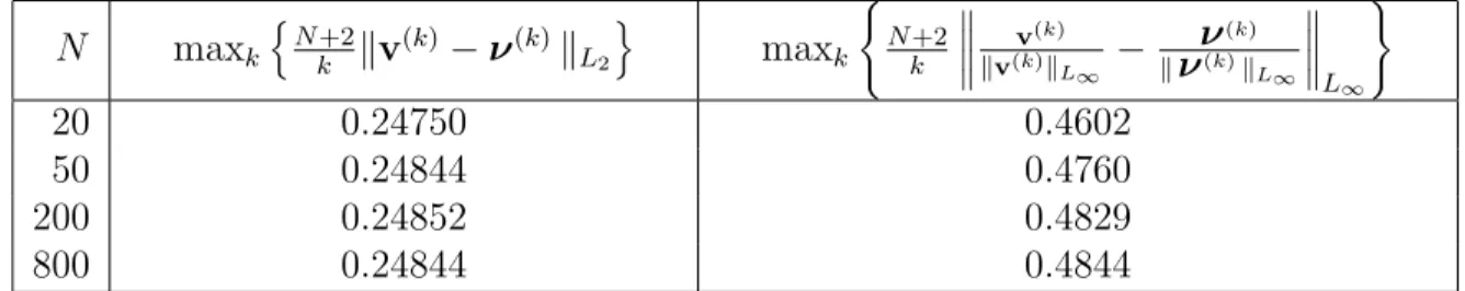
Numerical evaluation (see Table 1) shows that kv(k)_−ν(k)_k

L2 <

k

4(N+2)

for allk. The same rate of convergence is observed inL∞norm:

v(k) kv(k)_k L∞ − ν(k) kν(k)_k L∞ L∞ < k

2(N+2). (k·kL∞is the supremum norm in the time domain.) Figure 1 plots the

envelopes of |V(k)(f)|2 _{for both the minimum bias and sinusoidal tapers with}

N = 200, k = 1. The spectral energy of both tapers is nearly identical for

|f|< .25. Near the Nyquist frequency, the spectral energy of the sinusoidal taper is roughly three times larger than that of the minimum bias taper. In the time domain, the sinusoidal tapers are virtually indistinguishable from the MB tapers.

4

Comparison of Spectral Localizations

We now compare the local bias and the spectral concentration of three fam-ilies of orthonormal tapers: minimum bias (MB) tapers, sinusoidal tapers and Slepian tapers. Both the local bias and the spectral concentration of the

Slepian tapers depend on the bandwidth parameter, w. For properties of the Slepian tapers, we refer the reader to [12, 16, 17, 18, 19].

Since the MB tapers minimize the local bias, clearly the sinusoidal tapers and the Slepian tapers have larger local bias. The only question is whether the difference is large or small. Table 2 gives the local bias,PK

k=1

R1/2

−1/2f2|V(k)(f)|2df,

of the three families of tapers for N = 50. The sinusoidal tapers come within

0.2% of achieving the optimal local bias. In contrast, the local bias of the Slepian tapers can be many times larger.

We compute the local bias for three different values of the bandwidth,w.

The general pattern is that the kth Slepian taper has roughly the same local

bias as the MB taper does whenN w < k <2N w. The ratio of the local bias

of the Slepian tapers to that of the MB tapers is smallest atk ≈1.2N w. As

|k−1.2N w|increases, the local bias rapidly departs from the optimal value.

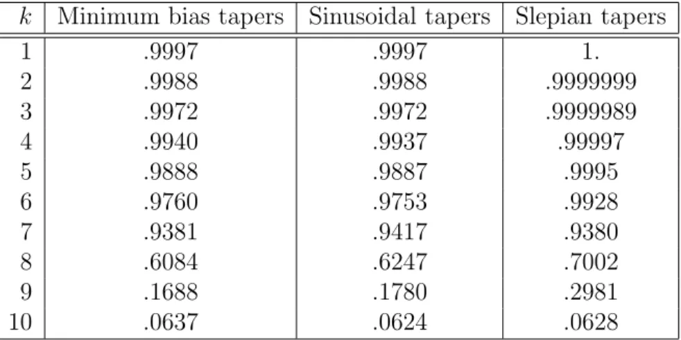
Table 3 compares the spectral concentration of the tapers forN = 50 and

w =.08 . Both the MB tapers and the sinusoidal tapers are within 1.7% of

the optimal value, except for k = 8,9. Notice that 2N w = 8. Although the

ratio of the spectral concentration, Rw

−w|V(f)|2df, for the MB and sinusoidal

tapers to that of the Slepian tapers is usually very close to one, the ratio of the spectral energy outside of the frequency band |f|< w can be quite large.

Thus our conclusions depend on usingRw

−w|V(f)|2df and not 1−

Rw

−w|V(f)|2df

as the measure of frequency concentration.

Figures 1-3 compare|V(k)_(f)|2 _{of the Slepian and MB tapers forN = 200.}

For Figures 1 and 2, we select the Slepian parameter, w, equal to .01 so that

K = 2N w equals four. Figure 2 plots |V1(f)|2 for the frequencies up to

f = 0.14. The central peak of the MB taper is more concentrated around

f = 0 than the Slepian taper is. The first sidelobe of the MB taper is visible

while the first Slepian sidelobe is much smaller.

Figure 1 plots the logarithm of |V1(f)|2 over the entire frequency range.

The MB taper has smaller range bias in the frequency range |f|<0.3w and

in the frequency range|f|>0.13. In the middle frequency range, the Slepian taper is clearly better. The Slepian penalty function maximizes the energy

inside the frequency band, [−w, w], and thus it is natural that the Slepian

tapers do better for f ∼ w. By using a discontinuous penalty function, the

Slepian spectral windows experience Gibbs phenomenon and decay only as

1

f, (|V(f)|

2 _∼ 1

f2). The MB spectral windows decay as

1

f2, and thus, it is

natural that the MB tapers have lower bias for f ∼ O(1).

Figure 3 plots P3

tapers are clearly preferable to the Slepian tapers. For larger frequencies, the

energy of the multitaper estimate, PK

k=1|V(k)(f)|2, is very similar to Fig. 2

on the logarithmic scale provided that K << N.

In summary, the sinusoidal tapers perform nearly as well as the MB tapers while the Slepian tapers have several times larger local bias (except when

k ≈1.2N w). For k 2N w, the Slepian tapers have better broad-band bias

protection than the minimum bias tapers do. For k ∼ 2N w, the minimum

bias tapers provide both smaller local bias and better broad-band protection due to the Gibbs phenomena which the Slepian tapers experience.

5

Local Error Analysis and Optimal

Multita-pering

We now give a local error analysis of MTSA and determine the optimal number of tapers. Our results are the multitaper analog of the local error analysis of the smoothed periodogram [4, 10]. We assume the time series is

a Gaussian processes and do not consider frequencies near f = 0 and f =

1/2. In this case, the variance of the multitaper estimate is approximately Variance[ ˆS(f)]≈S(f)2PK

k=1µ2k due to the orthonormality of the tapers

Asymptotically, the local bias of the multitaper estimate of Eq. (3) is

Bias[ ˆS] = S(f) K X k=1 µk−1 ! + 1 2S 00 (f) K X k=1 λkµk, where λk = R1/2 −1/2f

2_|V(k)_(f)|2_{df. The second term is the MT generalization}

of (7). When PK

k=1µk 6= 1, the MT estimate has bias even in white noise.

When we require PK

k=1µk= 1, the local expected loss simplifies:

Theorem 5.1 For a Gaussian process, away from f = 0 and f = 1/2, the expected square error of the multitaper spectral estimate (3) with PK

k=1µk = 1 is asymptotically (to leading order in K/N)

Bias2+ Variance ≈ " 1 2S 00 (f) K X k=1 λkµk #2 +S(f)2 K X k=1 µ2_k . (10)

Theorem 5.2 The multitaper estimate which minimizes the local loss (10) (with µk ≥0) is constructed with the minimum bias tapers.

Proof: We order theµk such that µ1 ≥µ2 ≥. . .≥µK and defineµK+1 =

0. Since the weights, µk are fixed, we need to minimize PKk=1µkukA u∗k

over all sets of K orthonormal tapers, u1, . . . ,uK. We split the series in K

subseries and minimize each subseries separately: min u1,...,uK K X k=1 µkukA u∗k = _umin 1,...,uK K X k=1 (µk−µk−1)   k X j=1 ujA u∗j   ≥ K X k=1 (µk−µk−1)   min u(₁k),...,u(_kk) k X j=1 u(_jk)A u(_jk)∗   = K X k=1 (µk−µk−1)   k X j=1 λA,j   = K X k=1 µkλA,j, (11)

where the λA,j are the eigenvalues of A, given in increasing order. The

u(_jk) are subject to orthonormality constraints thatu(_jk)·u(_jk0) =δ_j,j0, but are

otherwise independent and minimized separately. In the last line of (11), we use Fan’s Theorem [6]: min

u(₁k),...,u(_kk) Pk j=1u (k) j A u (k)∗ j = Pk

j=1λA,j, where the

u(_jk) are again subject to orthonormality constraints. The theorem is now

proved because the MB tapers are precisely the eigenvectors of A.

Theorem 5.3 The uniformly weighted multitaper estimate using K sinu-soidal tapers has an asymptotic local loss of

Bias2+ Variance ' " S00(f)K2 24N2 #2 + S(f) 2 K . (12)

Corollary 5.4 The asymptotic local loss of (12) is minimized when the num-ber of tapers is chosen as

Kopt ∼ " 12S(f)N2 S00_(f) #2/5 . (13)

Thus, the optimal number of tapers is proportional to N4/5 _{and varies}

with the ratio of S(f) to S00(f). Intuitively (13) shows that fewer tapers

should be used when the spectrum varies more rapidly. A key advantage of the MB and sinusoidal tapers is that the tapers need not be recomputed

as K is changed. In contrast, the Slepian tapers are most efficient when

the bandwidth parameter, w, is chosen such that K ∼ 2N w. Thus, when

the number of tapers is changed, as in (13), the Slepian tapers should be recomputed.

6

Smoothed Multitaper Estimates

In our own comparison of kernel smoothing and multitaper estimation [16], we found that a smoothed multiple taper estimate worked best. We now evaluate the expected error of the kernel smoothed multitaper estimator and show that smoothing the logarithm of the multitaper estimate is useful for

estimating the logarithm of the spectrum.

We begin by evaluating that the quadratic estimator (2) which is

equiv-alent to a kernel smoother estimates of the spectrum [4, 10]. Let ˆS(f) be

the quadratic spectral estimator (2), and smooth it with a kernel κ(·) of

halfwidth w : b b S(f) = Z w −w κ(g w)S(fb +g)dg , (14)

where w is the bandwidth parameter and κ(·) is a kernel smoother with

domain [−1,1]. This can be rewritten as

b_b S(f) = N X n,m=1 ˜ qnmei2π(m−n)fxnxm , (15) where ˜qnm = qnmˆκm−n with ˆκm = Rw

−wκ(g/w)e2πimgdg. Thus

smooth-ing replaces the original quadratic estimator with matrix [qnm] by another

quadratic estimator with matrix ˜Q = [˜qnm]. By Theorem 5.2, this hybrid

method cannot outperform the pure multitaper method with minimum bias tapers.

We now show that combining kernel smoothing with multitapering does

improve the estimation of the logarithm of the spectral density, θ(f) =

log[S(f)]. One standard approach is to kernel smooth the logarithm of the

tapered periodogram. This approach has the disadvantage that|y(f)|2 _{has a}

χ2

2 distribution and log[χ22] has a long lower tail of its distribution. As a

re-sult, log[|y(f)|2_{] has an appreciable bias and its variance is inflated by π}2_/6.

A common alternative is to estimate the spectrum either by kernel smoothing or by multitapering and then to take logarithms. This approach has the dis-advantage that the smoothed spectral estimate tends to be more sensitive to nonlocal bias effects than the corresponding smoothed log-spectral estimate. To robustify the log-spectral estimate while reducing the variance infla-tion from the long tail, we propose the following hybrid estimate: 1) compute

the multitaper estimate using the sinusoidal tapers with µk = _K1 and then

(BK ≡ ψ(K)−lnK whereψ(K) is the digamma function). For white noise,

the variance of ˆθM T(f) = ψ0(K)∼ _K1 + _2K12, so the variance enhancement

from the logarithm tends rapidly to zero.

In [15], we show that the asymptotic error for this scheme is

θ00(f)2 " bkw2+ K2 24N2 #2 + Cκ N w 1 + 1 2K 2 , (16)

wherebκ andCκ are constants which depend on the kernel shape. In (16), we

assume uniformly weighted sinusoidal tapers are used and 1 K N w. In

(16), one factor of (1 +₂1_K) is the variance enhancement from the logarithmic

transformation and one factor of (1 + ₂1_K) arises in the variance calculation

of (15) with sinusoidal tapers. Optimizing (16) with respect to both w and

K yieldw∼N−1/5 _{and K ∼N}8/15_{, thus the smoothing halfwidthwis much}

larger than K/N. The expected error (16) depends weakly on K provided

that 1K N w.

For simplicity, we set K = N8/15 _{and optimize (16) with respect to the}

halfwidth w. The resulting halfwidth depends on θ00(f): wopt(θ00(f)) with

wopt ∼ |θ00(f)|−2/5N−1/5. Thus when the log-spectrum varies rapidly, the

halfwidth should be reduced as |θ00(f)|−2/5_.

Sinceθ00(f) is unknown, we consider two stage estimators which begin by

making a preliminary estimate of θ00(f) prior to estimating θ(f). We then

insert the estimateθ00d(f) into the expression forw_opt: w(f) = w_opt(θc00(f)) and

use a variable halfwidth kernel smoother with halfwidth ˆw(f) to estimate

θ(f). Multiple stage kernel estimators are described in [2, 7, 13, 14, 15].

These multiple stage schemes have a convergence rate of N−4/5 and have a

relative convergence rate of at least N−2/9_{. A more detailed description is}

given in [2, 13, 15].

7

Application

We now compare spectral estimates on an actual data series. We use the microwave scattering data set which is described in [16]. The data measures turbulent plasma fluctuations in the Tokamak Fusion Test Reactor at Prince-ton. The spectrum is dominated by a 1 MHz peak which is quasicoherent. The spectral density varies by over five orders of magnitude.

The bias versus variance trade-off of Sec. 5 shows that fewer tapers should be used near the peak. To make the spectral estimate smooth, a parabolic weighting of the tapers is used as described in Sec. 3. To determine how many tapers to use locally, we use the multiple stage “plug-in” method as described in the previous section; i.e. we determine the number of tapers using a pre-estimate on the same data. To reduce the fluctuations from the estimate of the optimal number, we use a longer data segment to determine the number of tapers at each frequency. We find the optimal number of sinusoidal tapers is roughly 24 for frequencies in the 200 to 800 kHz range. Near the 1 MHz peak, as few as 12 tapers are used to minimize the local bias error. Between 1300 and 2400 kHz, the spectrum is flatter and we use up to 40 tapers.

The dotted line is the sinusoidal multitaper estimate, and the solid, more wiggly, curve is the corresponding Slepian estimate using 24 tapers with

w= 60 kHz. The 1 MHz peak is poorly resolved in the Slepian estimate, and

the regions of high curvature are artificially flattened. For f ≥1.5 MHz, the

Slepian estimate is artificially bumpy due to statistical noise. The variable taper number estimate suppresses these bumps by averaging over a larger frequency halfwidth. We have also used a variable taper number estimate

with the Slepian tapers. Since the Slepian parameter,wwas fixed at 100 kHz

to allow for forty tapers, the artificial broadening was even more exreme.

Comparing with a converged estimate of the spectrum based on N =

45,000 shows that the sinuosidal taper estimate is more accurate. Another

significant difference is that the Slepian multitaper estimate requires much more CPU time than the sinusoidal multitaper estimate.

8

Conclusion

We have proposed and analyzed the minimum bias and the sinusoidal tapers, v(k)

n =

q ₂

N+1sin

πkn

N+1, for multitaper spectral estimation. The resulting

sinu-soidal multitaper spectral estimate is ˆS(f) = _2K(N1₊₁₎PK

j=1|y(f +

j

2N+2)−

y(f − _2Nj₊₂)|2_{. The sinusoidal tapers have low bias because the frequency}

sidelobe from y(f +_2Nj₊₂) cancels the sidelobe of y(f− j

2N+2).

The minimum bias tapers minimize the local bias, R1/2

−1/2f

2_|V(k)_b(f)|2_df,

and have good broad-band bias protection as well. Asymptotically, the

er-ror is a multiple taper estimate using the minimal bias tapers.

The sinusoidal tapers have a simple analytic form and approximate the

minimum bias tapers to O1

N

. The kth sinusoidal taper has its spectral

energy concentrated in the frequency bands ₂₍k_N−₊₁₎1 ≤ |f| ≤ k+1 2(N+1).

The minimum bias and sinusoidal tapers have no auxiliary bandwidth pa-rameter, and the bandwidth of the spectral estimate is determined solely by the number of used tapers. By adaptively adding and deleting tapers, a mul-titaper estimate with the optimal convergence properties of kernel smoothers can be constructed. In contrast, the Slepian tapers need to be recomputed with a different bandwidth. Thus the Slepian tapers are only practical for fixed bandwidth estimation and this is inherently inefficient.

9

Appendix: Multitaper decomposition of

ker-nel estimates

In Sec. 6, we showed that kernel smoother estimators (14) have an equivalent multitaper representation (3) We now show that the equivalent multitapers of some popular kernel smoother estimates of the spectrum strongly resemble the MB/sinusoidal tapers. In one special case, this corresondence is exact; i.e. the smoothed periodogram can be exactly decomposed into MB tapers.

Theorem 9.1 Let w= 1₂ and κ(f) be the parabolic kernel, κ(f) = 3₂ −6f2_.

The eigenvectors of the kernel smoothed periodogram are exactly the discrete minimum bias tapers.

Proof: The ˜Q matrix in (15) can be calculated explicitly for this case.

We find ˜Q = [bnm] = _N1(3₂I −6A) where A is the matrix from Lemma 3.2.

Thus ˜Q and A have the same eigenvectors.

To illustrate that this result is typical even when we apply a taper and smooth over a small band, we consider a smoothed tapered periodogram

with N = 200. We use Tukey’s split-cosine taper [16] and then smooth the

estimate with a square box kernel with a halfwidth of .01. We then evaluate

the corresponding ˜Q matrix and compute its eigenvectors. Figure 5 displays

the first 4 eigenvectors. They are very close to the sinusoids q_N2₊₁sin_Nπkn₊₁.

spectral estimate. After k > 4, the eigenvalues decrease sharply, and these higher eigenvectors contribute very little to the overall estimate.

References

[1] M. Amin, “Optimal estimation of evolutionary spectra,”

I.E.E.E. Trans. on Signal Processing vol. 42, 2?, 1994.

[2] T. Brockman, Th. Gasser and E. Hermann, “Locally adaptive

bandwidth choice for kernel regression estimators,”J. Amer. Stat.

Assoc. 88, 1302-1309 (1994).

[3] T. P. Bronez, Nonparametric Spectral Estimation of Irregularly

Sampled Multidimensional Random Processes, PhD Thesis, Ari-zona State University, 1985.

[4] U. Grenander and M. Rosenblatt,Statistical Analysis of

Station-ary Time Series, New York: Wiley, 1957.

[5] A. N. Kolmogorov and S. V. Fomin,Reele Funktionen und

Funk-tionalanalysis, Section 7.3.2, Berlin: VEB Deutscher Verlag der Wissenschaften, 1975.

[6] A. W. Marshall and I. Olkin,Inequalities: Theory of Majorization

and its Applications, p. 511, New York: Academic Press 1979.

[7] H.-G. M¨uller and U. Stadtm¨uller, “Variable bandwidth kernel

estimators of regression curves,” Annals of Statistics, vol. 15, pp. 182-201, 1987.

[8] C. T. Mullis and L. L. Scharf, inAdvances in Spectrum Analysis,

S. Haykin, Ed., New York: Prentice-Hall, 1990, Chapter 1, pp. 1-57.

[9] A. Papoulis, “Minimum bias windows for high resolution spectral

estimates,” IEEE Trans. Information Theory, vol. 19, pp. 9-12,

1973.

[10] E. Parzens, “On asymptotically efficient consistent estimates

of the spectral density of a stationary time series,” J. Royal

[11] J. Park, C. R. Lindberg, and F. L. Vernon, “Multitaper Spectral

analysis of high frequency seismograms,” J. Geophys. Res., vol.

92B, pp. 12765-12684, 1987.

[12] D. Percival and A. Walden, Spectral Analysis for Physical

Ap-plications: Multitaper and Conventional Univariate Techniques. Cambridge: Cambridge University Press, 1993.

[13] K. S. Riedel, “Optimal kernel estimation of evolutionary spectra,”

I.E.E.E. Trans. on Signal Processing vol. 41, 2439-2447, 1993. [14] K.S. Riedel and A. Sidorenko, “Function estimation using data

adaptive kernel smoothers- How much smoothing?” Computers

in Physics vol. 8, 402-409, 1994.

[15] K. S. Riedel and A. Sidorenko, “Smoothed log-multitaper spec-tral estimation and data adaptive implementation,” submitted for publication.

[16] K. S. Riedel, A. Sidorenko, and D. J. Thomson, “Spectral density estimation for plasma fluctuations I: Comparison of methods,”

Physics of Plasmas vol. 1, pp. 485-500.

[17] D. Slepian, “Prolate spheroidal wave functions, Fourier analysis,

and uncertainty - V: the discrete case,”Bell System Tech. J., vol.

5, pp. 1371-1429, 1978.

[18] D. J. Thomson, “Spectrum estimation and harmonic analysis,”

Proc. IEEE, vol. 70, pp. 1055-1096, 1982.

[19] D. J. Thomson, “Quadratic inverse spectrum estimates:

appli-cations to paleoclimatology,” Phil. Trans. R. Soc. Lond. A, vol.

Table Captions:

Table 1: Convergence of the sinusoidal tapers to the minimum bias tapers.

Table 2: Normalized bias term, 4(N + 1)2PK

k=1 R1/2 −1/2f2 PK k=1f2|V(k)(f)|2df, for N = 50.

Table 3: Spectral concentration, Rw

−w

PK

k=1|V(k)(f)|2df, for N = 50.

Table 4: Eigenvectors of the smooth tapered periodogram estimator.

Figure Captions:

Figure 1: Spectral energy of the minimum bias, sinusoidal and Slepian tapers,

N = 200, k = 1, w =.01.

Figure 2: Spectral energy of the minimum bias and sinusoidal tapers,N = 200, k= 1.

Figure 3 Spectral energy,P3

k=1

R1/2

−1/2f

2_|V(k)_(f)|2_{df, of the minimum bias and}

Slepian tapers, N = 200, K = 3, w =.01.

Figure 4: Estimated spectral density of the plasma fluctuations. Dashed line is sinusoidal multitaper estimate and solid line is estimate using Slepian

tapers with w= 60 kHz. Because the Slepian tapers have a fixed bandwidth,

the corresponding estimate spectral density at 1 MHz is artificially broadened

while being undersmoothed for f ≥1.5 MHz.

Figure 6: First eigenvectors of the smooth tapered periodogram estima-tor.

Table 1. Convergence of the sinusoidal tapers to the minimum bias tapers N maxk n_N+2 k kv (k)_−ν(k)_k L2 o maxk ( N+2 k v(k) kv(k)_k L∞ − ν(k) kν(k)_k L∞ _L ∞ ) 20 0.24750 0.4602 50 0.24844 0.4760 200 0.24852 0.4829 800 0.24844 0.4844

Table 2. Normalized bias term, 4(N + 1)2PK

k=1

R1/2

−1/2f

2_|V(k)_(f)|2_{df, for}

N = 50

K Minimum Sinusoidal Slepian tapers

bias tapers tapers w=0.04 w=0.08 w=0.16

1 1.0095 1.0116 1.3439 2.6316 5.1039 2 5.0475 5.0580 5.7724 10.5484 20.4670 3 14.1328 14.1622 18.0651 23.8086 46.1953 4 30.2846 30.3475 58.9520 42.5181 82.4018 5 55.5217 55.6366 154.4818 66.9996 129.2087 6 91.8634 92.0528 305.4382 99.1800 186.7507 7 141.3284 141.6185 496.7959 150.0103 255.1797 8 205.9362 206.3570 721.1743 251.8833 334.6717 9 287.7056 288.2899 976.5088 437.5993 425.4379 10 388.6562 389.4409 1262.4251 702.1523 527.7433

Table 3. Spectral concentration, Rw

−w|V(f)|2df, forN = 50, w = 0.08

k Minimum bias tapers Sinusoidal tapers Slepian tapers

1 .9997 .9997 1. 2 .9988 .9988 .9999999 3 .9972 .9972 .9999989 4 .9940 .9937 .99997 5 .9888 .9887 .9995 6 .9760 .9753 .9928 7 .9381 .9417 .9380 8 .6084 .6247 .7002 9 .1688 .1780 .2981 10 .0637 .0624 .0628

Table 4. Eigenvectors of the smooth tapered periodogram estimator

k Weight of the eigenvector Normalized local bias Local bias in comparison with

λk(B)/tr(B) 4(N + 1)2R

1/2

−1/2f

2_|V(f)|2_{df the minimum bias taper (ratio)}

1 .2856 1.5138 1.509 2 .2828 4.7371 1.181 3 .2519 9.6254 1.067 4 .1416 19.2095 1.198 5 .0340 33.7118 1.345 6 .0037 51.3616 1.423 7 .0002 72.9747 1.486