Predicting Good Probabilities With Supervised Learning

(1)

Predicting Good Probabilities With Supervised Learning

Alexandru Niculescu-Mizil ALEXN@CS.CORNELL.EDU

Rich Caruana CARUANA@CS.CORNELL.EDU

Department Of Computer Science, Cornell University, Ithaca NY 14853

Abstract

We examine the relationship between the predic-tions made by different learning algorithms and true posterior probabilities. We show that maxi-mum margin methods such as boosted trees and boosted stumps push probability mass away from 0 and 1 yielding a characteristic sigmoid shaped distortion in the predicted probabilities. Mod-els such as Naive Bayes, which make unrealis-tic independence assumptions, push probabilities toward 0 and 1. Other models such as neural nets and bagged trees do not have these biases and predict well calibrated probabilities. We ex-periment with two ways of correcting the biased probabilities predicted by some learning meth-ods: Platt Scaling and Isotonic Regression. We qualitatively examine what kinds of distortions these calibration methods are suitable for and quantitatively examine how much data they need to be effective. The empirical results show that after calibration boosted trees, random forests, and SVMs predict the best probabilities.

1. Introduction

In many applications it is important to predict well cali-brated probabilities; good accuracy or area under the ROC curve are not sufficient. This paper examines the prob-abilities predicted by ten supervised learning algorithms: SVMs, neural nets, decision trees, memory-based learn-ing, bagged trees, random forests, boosted trees, boosted stumps, naive bayes and logistic regression. We show how maximum margin methods such as SVMs, boosted trees, and boosted stumps tend to push predicted probabilities away from 0 and 1. This hurts the quality of the probabili-ties they predict and yields a characteristic sigmoid-shaped distortion in the predicted probabilities. Other methods such as naive bayes have the opposite bias and tend to push predictions closer to 0 and 1. And some learning methods

Appearing in Proceedings of the22nd_{International Conference}

such as bagged trees and neural nets have little or no bias and predict well-calibrated probabilities.

After examining the distortion (or lack of) characteristic to each learning method, we experiment with two calibration methods for correcting these distortions.

Platt Scaling: a method for transforming SVM outputs

from[−∞,+∞]to posterior probabilities (Platt, 1999)

Isotonic Regression: the method used by Zadrozny and

Elkan (2002; 2001) to calibrate predictions from boosted naive bayes, SVM, and decision tree models

Platt Scaling is most effective when the distortion in the predicted probabilities is sigmoid-shaped. Isotonic Regres-sion is a more powerful calibration method that can correct any monotonic distortion. Unfortunately, this extra power comes at a price. A learning curve analysis shows that Iso-tonic Regression is more prone to overfitting, and thus per-forms worse than Platt Scaling, when data is scarce. Finally, we examine how good are the probabilities pre-dicted by each learning method after each method’s predic-tions have been calibrated. Experiments with eight classi-fication problems suggest that random forests, neural nets and bagged decision trees are the best learning methods for predicting well-calibrated probabilities prior to calibration, but after calibration the best methods are boosted trees, ran-dom forests and SVMs.

2. Calibration Methods

In this section we describe the two methods for mapping model predictions to posterior probabilities: Platt Calibra-tion and Isotonic Regression. Unfortunately, these methods are designed for binary classification and it is not trivial to extend them to multiclass problems. One way to deal with multiclass problems is to transform them to binary prob-lems, calibrate the binary models, and recombine the pre-dictions (Zadrozny & Elkan, 2002).

2.1. Platt Calibration

Platt (1999) proposed transforming SVM predictions to posterior probabilities by passing them through a sigmoid. We will see in Section 4 that a sigmoid transformation is

(2)

also justified for boosted trees and boosted stumps. Let the output of a learning method bef(x). To get cali-brated probabilities, pass the output through a sigmoid:

P(y= 1|f) = 1

1 +exp(Af+B) (1)

where the parametersAandB are fitted using maximum likelihood estimation from a fitting training set (fi, yi).

Gradient descent is used to find A andB such that they are the solution to:

argmin

A,B

{−X

i

yilog(pi) + (1−yi)log(1−pi)}, (2)

where

pi=

1

1 +exp(Afi+B)

(3)

Two questions arise: where does the sigmoid train set come from? and how to avoid overfitting to this training set? If we use the same data set that was used to train the model we want to calibrate, we introduce unwanted bias. For ex-ample, if the model learns to discriminate the train set per-fectly and orders all the negative examples before the posi-tive examples, then the sigmoid transformation will output just a 0,1 function. So we need to use an independent cali-bration set in order to get good posterior probabilities. This, however, is not a draw back, since the same set can be used for model and parameter selection.

To avoid overfitting to the sigmoid train set, an out-of-sample model is used. If there areN+positive examples

andN− negative examples in the train set, for each train-ing example Platt Calibration uses target valuesy+andy₋

(instead of 1 and 0, respectively), where y+=

N++ 1

N++ 2

; y−=

1

N₋+ 2 (4)

For a more detailed treatment, and a justification of these particular target values see (Platt, 1999).

2.2. Isotonic Regression

The sigmoid transformation works well for some learning methods, but it is not appropriate for others. Zadrozny and Elkan (2002; 2001) successfully used a more general method based on Isotonic Regression (Robertson et al., 1988) to calibrate predictions from SVMs, Naive Bayes, boosted Naive Bayes, and decision trees. This method is more general in that the only restriction is that the mapping function be isotonic (monotonically increasing). That is, given the predictionsfi from a model and the true targets

yi, the basic assumption in Isotonic Regression is that:

yi=m(fi) +i (5)

Table 1. PAV Algorithm

Algorithm 1. PAV algorithm for estimating posterior

probabilities from uncalibrated model predictions. 1 Input: training set(fi, yi)sorted according tofi

2 Initializemˆi,i=yi,wi,i= 1

3 While∃i s.t.mˆk,i−1≥mˆi,l Setwk,l=wk,i−1+wi,l

Setmˆk,l= (wk,i−1mˆk,i−1+wi,lmˆi,l)/wk,l Replacemˆk,i−1andmˆi,lwithmˆk,l

4 Output the stepwise const. function:

ˆ

m(f) = ˆmi,j, forfi< f≤fj

where m is an isotonic (monotonically increasing) func-tion. Then, given a train set(fi, yi), the Isotonic

Regres-sion problem is finding the isotonic functionmˆ such that

ˆ

m=argminz X

(yi−z(fi))2 (6)

One algorithm that finds a stepwise constant solution for the Isotonic Regression problem is pair-adjacent violators (PAV) algorithm (Ayer et al., 1955) presented in Table 1. As in the case of Platt calibration, if we use the model train-ing set(xi, yi)to get the training set(f(xi), yi)for Isotonic

Regression, we introduce unwanted bias. So we use an in-dependent validation set to train the isotonic function.

3. Data Sets

We compare algorithms on 8 binary classification prob-lems. ADULT, COV TYPE and LETTER are from UCI Repository (Blake & Merz, 1998). COV TYPE has been converted to a binary problem by treating the largest class as positive and the rest as negative. We converted LETTER to boolean two ways. LETTER.p1 treats the letter ”O” as positive and the remaining 25 letters as negative, yielding a very unbalanced problem. LETTER.p2 uses letters A-M as positives and N-Z as negatives, yielding a difficult, but well balanced, problem. HS is the IndianPine92 data set (Gualtieri et al., 1999) where the difficult class Soybean-mintill is the positive class. SLAC is a problem from the Stanford Linear Accelerator. MEDIS and MG are medical data sets. The data sets are summarized in Table 2.

Table 2. Description of problems

PROBLEM #ATTR TRAIN SIZE TEST SIZE %POZ

ADULT 14/104 4000 35222 25%

COV TYPE 54 4000 25000 36%

LETTER.P1 16 4000 14000 3%

LETTER.P2 16 4000 14000 53%

MEDIS 63 4000 8199 11%

MG 124 4000 12807 17%

SLAC 59 4000 25000 50%

(3)

4. Qualitative Analysis of Predictions

In this section we qualitatively examine the calibration of the different learning algorithms. For each algorithm we use many variations and parameter settings to train differ-ent models. For example, we train models using ten de-cision tree styles, neural nets of many sizes, SVMs with many kernels, etc. After training, we apply Platt Scal-ing and Isotonic Regression to calibrate all models. Each model is trained on the same random sample of 4000 cases and calibrated on independent samples of 1000 cases. For the figures in this section we select, for each problem, and for each learning algorithm, the model that has the best cal-ibration before or after scaling.

On real problems where the true conditional probabilities are not known, model calibration can be visualized with re-liability diagrams (DeGroot & Fienberg, 1982). First, the prediction space is discretized into ten bins. Cases with predicted value between 0 and 0.1 fall in the first bin, be-tween 0.1 and 0.2 in the second bin, etc. For each bin, the mean predicted value is plotted against the true fraction of positive cases. If the model is well calibrated the points will fall near the diagonal line.

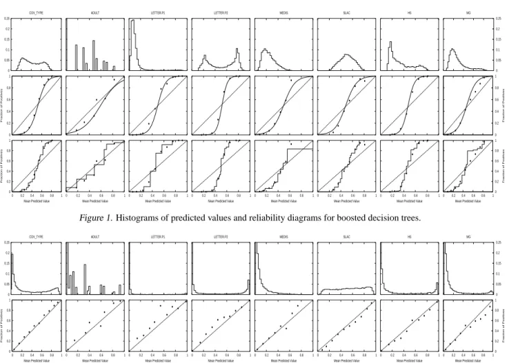
We first examine the predictions made by boosted trees. Figure 1 shows histograms of the predicted values (top row) and reliability diagrams (middle and bottom rows) for boosted trees on the eight test problems on large test sets not used for training or calibration. An interesting aspect of the reliability plots in Figure 1 is that they display a sig-moidal shape on seven of the eight problems1, motivating the use of a sigmoid to transform predictions into calibrated probabilities. The reliability plots in the middle row of the figure show sigmoids fitted using Platt’s method. The reli-ability plots in the bottom of the figure show the function fitted with Isotonic Regression.

Examining the histograms of predicted values (top row in Figure 1), note that almost all the values predicted by boosted trees lie in the central region with few predictions approaching 0 or 1. The one exception is LETTER.P1, a highly skewed data set that has only 3% positive class. On this problem some predicted values do approach 0, though careful examination of the histogram shows that even on this problem there is a sharp drop in the number of cases predicted to have probability near 0. This shifting of the predictions toward the center of the histogram causes the sigmoid-shaped reliability plots of boosted trees.

To show how calibration transforms predictions, we plot histograms and reliability diagrams for the eight problems

1

Because boosting overfits on the ADULT problem, the best performance is achieved after only four iterations of boosting. If boosting is allowed to continue for more iterations, it will display the same sigmoidal shape on ADULT as in the other figures.

for boosted trees after Platt Calibration (Figure 2) and Iso-tonic Regression (Figure 3). The figures show that calibra-tion undoes the shift in probability mass caused by boost-ing: after calibration many more cases have predicted prob-abilities near 0 and 1. The reliability diagrams are closer to diagonal, and the S-shape characteristic of boosted tree predictions is gone. On each problem, transforming pre-dictions using Platt Scaling or Isotonic Regression yields a significant improvement in the predicted probabilities, leading to much lower squared error and log-loss. One difference between Isotonic Regression and Platt Scaling is apparent in the histograms: because Isotonic Regression generates a piecewise constant function, the histograms are coarse, while the histograms generated by Platt Scaling are smoother. See (Niculescu-Mizil & Caruana, 2005) for a more thorough analysis of boosting from the point-of-view of predicting well-calibrated probabilities.

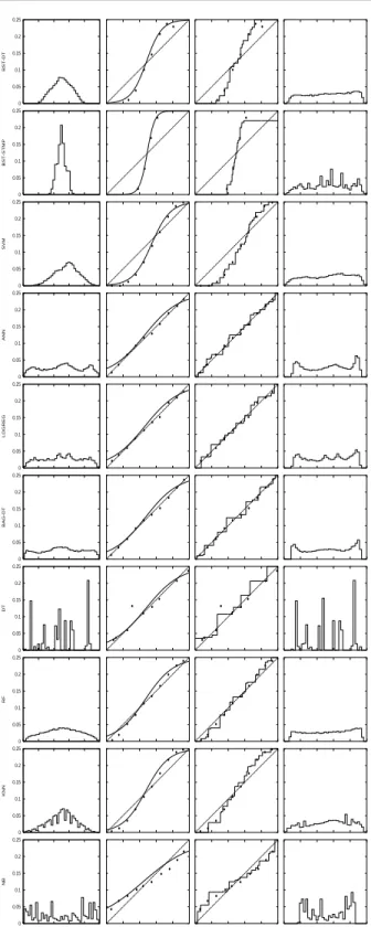
Figure 6 shows the prediction histograms for the ten learn-ing methods on the SLAC problem before calibration, and after calibration with Platt’s method. Reliability diagrams showing the fitted functions for Platt’s method and Iso-tonic Regression also are shown. Boosted stumps and SVMs2 also exhibit distinctive sigmoid-shaped reliability plots (second and third rows, respectively, of Figure 6). Boosted stumps and SVMs exhibit similar behavior on the other seven problems. As in the case of boosted trees, the sigmoidal shape of the reliability plots co-occurs with the concentration of mass in the center of the histograms of predicted values, with boosted stumps being the most ex-treme. It is interesting to note that the learning methods that exhibit this behavior are maximum margin methods. The sigmoid-shaped reliability plot that results from pre-dictions being pushed away from 0 and 1 appears to be characteristic of max margin methods.

Figure 4 which shows histograms of predicted values and reliability plots for neural nets tells a very different story. The reliability plots closely follow the diagonal line indi-cating that neural nets are well calibrated to begin with and do not need post-training calibration. Only the COV TYPE problem appears to benefit a little from calibration. On the other problems both calibration methods appear to be striv-ing to approximate the diagonal line, a task that isn’t nat-ural to either of them. Because of this, scaling might hurt neural net calibration a little. The sigmoids trained with Platt’s method have trouble fitting the tails properly, effec-tively pushing predictions away from 0 and 1 as can be seen in the histograms in Figure 5. The histograms for uncali-brated neural nets in Figure 4 look similar to the histograms for boosted trees after Platt Scaling in Figure 2, giving us confidence that the histograms reflect the underlying

struc-2

SVM predictions are scaled to [0,1] by(x−min)/(max−

(4)

0 0.05 0.1 0.15 0.2 0.25

COV_TYPE ADULT LETTER.P1 LETTER.P2 MEDIS SLAC HS

0 0.05 0.1 0.15 0.2 0.25 MG

0 0.2 0.4 0.6 0.8 1

Fraction of Positives

0 0.2 0.4 0.6 0.8 1

Mean Predicted Value

0 0.2 0.4 0.6 0.8 1 Mean Predicted Value

0 0.2 0.4 0.6 0.8 1 0 0.2 0.4 0.6 0.8 1

Figure 1. Histograms of predicted values and reliability diagrams for boosted decision trees.

0 0.05 0.1 0.15 0.2 0.25

0 0.05 0.1 0.15 0.2 0.25 MG

0 0.2 0.4 0.6 0.8 1

0 0.2 0.4 0.6 0.8 1 0 0.2 0.4 0.6 0.8 1

Figure 2. Histograms of predicted values and reliability diagrams for boosted trees calibrated with Platt’s method.

0 0.05 0.1 0.15 0.2 0.25

0 0.05 0.1 0.15 0.2 0.25 MG

0 0.2 0.4 0.6 0.8 1

0 0.2 0.4 0.6 0.8 1 0 0.2 0.4 0.6 0.8 1

Figure 3. Histograms of predicted values and reliability diagrams for boosted trees calibrated with Isotonic Regression.

ture of the problems. For example, we could conclude that the LETTER and HS problems, given the available fea-tures, have well defined classes with a small number of cases in the “gray” region, while in the SLAC problem the two classes have high overlap with significant uncertainty for most cases. It is interesting to note that neural networks with a single sigmoid output unit can be viewed as a linear classifier (in the span of it’s hidden units) with a sigmoid at the output that calibrates the predictions. In this respect

neural nets are similar to SVMs and boosted trees after they have been calibrated using Platt’s method.

Examining the histograms and reliability diagrams for lo-gistic regression and bagged trees shows that they be-have similar to neural nets. Both learning algorithms are well calibrated initially and post-calibration does not help them on most problems. Bagged trees are helped a little by post-calibration on the MEDIS and LETTER.P2 prob-lems. While it is not surprising that logistic regression

(5)

0 0.05 0.1 0.15 0.2 0.25

0 0.05 0.1 0.15 0.2 0.25 MG

0 0.2 0.4 0.6 0.8 1

0 0.2 0.4 0.6 0.8 1 0 0.2 0.4 0.6 0.8 1

Figure 4. Histograms of predicted values and reliability diagrams for neural nets.

0 0.05 0.1 0.15 0.2 0.25

0 0.05 0.1 0.15 0.2 0.25 MG

0 0.2 0.4 0.6 0.8 1

0 0.2 0.4 0.6 0.8 1 0 0.2 0.4 0.6 0.8 1

Figure 5. Histograms of predicted values and reliability diagrams for neural nets calibrated with Platt’s method.

dicts such well-calibrated probabilities, it is interesting that bagging decision trees also yields well-calibrated models. Given that bagged trees are well calibrated, we can deduce that regular decision trees also are well calibrated on aver-age, in the sense that if decision trees are trained on dif-ferent samples of the data and their predictions averaged, the average will be well calibrated. Unfortunately, a sin-gle decision tree has high variance and this variance affects it’s calibration. Platt Scaling is not able to deal with this high variance, but Isotonic Regression can help fix some of the problems created by variance. Rows five, six and seven in Figure 6 show the histograms (before and after calibration) and reliability diagrams for logistic regression, bagged trees, and decision trees on the SLAC problem. Random forests are less clear cut. RF models are well calibrated on some problems, but are poorly calibrated on LETTER.P2, and not well calibrated on HS, COV TYPE, MEDIS and LETTER.P1. It is interesting that on these problems, RFs seem to exhibit, although to a lesser ex-tent, the same behavior as the max margin methods: pre-dicted values are slightly pushed toward the middle of the histogram and the reliability plots show a sigmoidal shape

(more accentuated on the LETTER problems and less so on COV TYPE, MEDIS and HS). Methods such as bagging and random forests that average predictions from a base set of models can have difficulty making predictions near 0 and 1 because variance in the underlying base models will bias predictions that should be near zero or one away from these values. Because predictions are restricted to the in-terval [0,1], errors caused by variance tend to be one-sided near zero and one. For example, if a model should predict p= 0for a case, the only way bagging can achieve this is if all bagged trees predict zero. If we add noise to the trees that bagging is averaging over, this noise will cause some trees to predict values larger than 0 for this case, thus mov-ing the average prediction of the bagged ensemble away from 0. We observe this effect most strongly with random forests because the base-level trees trained with random forests have relatively high variance due to feature subset-ting. Post-calibration seems to help mitigate this problem. Because Naive Bayes makes the unrealistic assumption that the attributes are conditionally independent given the class, it tends to push predicted values toward 0 and 1. This is the opposite behavior from the max margin methods and

(6)

0 0.05 0.1 0.15 0.2 0.25

BST-DT

0 0.05 0.1 0.15 0.2 0.25

BST-STMP

0 0.05 0.1 0.15 0.2 0.25

SVM

0 0.05 0.1 0.15 0.2 0.25

ANN

0 0.05 0.1 0.15 0.2 0.25

LOGREG

0 0.05 0.1 0.15 0.2 0.25

BAG-DT

0 0.05 0.1 0.15 0.2 0.25

DT

0 0.05 0.1 0.15 0.2 0.25

RF

0 0.05 0.1 0.15 0.2 0.25

KNN

0 0.05 0.1 0.15 0.2 0.25

NB

Figure 6. Histograms and reliability diagrams for SLAC.

ates reliability plots that have an inverted sigmoid shape. While Platt Scaling is still helping to improve calibration, it is clear that a sigmoid is not the right transformation to calibrate Naive Bayes models. Isotonic Regression is a bet-ter choice to calibrate these models.

Returning to Figure 6, we see that the histograms of the pre-dicted values before calibration (first column) from the ten different models display wide variation. The max margin methods (SVM, boosted trees, and boosted stumps) have the predicted values massed in the center of the histograms, causing a sigmoidal shape in the reliability plots. Both Platt Scaling and Isotonic Regression are effective at fitting this sigmoidal shape. After calibration the prediction his-tograms extend further into the tails near predicted values of 0 and 1.

For methods that are well calibrated (neural nets, bagged trees, random forests, and logistic regression), calibration with Platt Scaling actually moves probability mass away from 0 and 1. It is clear from looking at the reliability di-agrams for these methods that the sigmoid has difficulty fitting the predictions in the tails of these well-calibrated methods.

Overall, if one examines the probability histograms before and after calibration, it is clear that the histograms are much more similar to each other after Platt Scaling. Calibration significantly reduces the differences between the probabil-ities predicted by the different models. Of course, calibra-tion is unable to fully correct the prediccalibra-tions from the infe-rior models such as decision trees and naive bayes.

5. Learning Curve Analysis

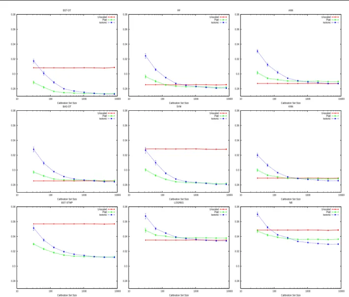
In this section we present a learning curve analysis of the two calibration methods, Platt Scaling and Isotonic Regres-sion. The goal is to determine how effective these calibra-tion methods are as the amount of data available for cali-bration varies. For this analysis we use the same models as in Section 4, but here we vary the size of the calibration set from 32 cases to 8192 cases by factors of two. To measure calibration performance we examine the squared error of the models.

The plots in Figure 7 show the average squared error over the eight test problems. For each problem, we perform ten trials. Error bars are shown on the plots, but are so nar-row that they may be difficult to see. Calibration learning curves are shown for nine of the ten learning methods (de-cision trees are left out).

The nearly horizontal lines in the graphs show the squared error prior to calibration. These lines are not perfectly horizontal only because the test sets change as more data is moved into the calibration sets. Each plot shows the squared error after calibration with Platt’s method or Iso-tonic Regression as the size of the calibration set varies from small to large. When the calibration set is small (less than about 200-1000 cases), Platt Scaling outperforms Iso-tonic Regression with all nine learning methods. This hap-pens because Isotonic Regression is less constrained than

(7)

0.28 0.3 0.32 0.34 0.36 0.38

10 100 1000 10000

Calibration Set Size BST-DT

Unscaled Platt Isotonic

0.28 0.3 0.32 0.34 0.36 0.38

10 100 1000 10000

Calibration Set Size RF

0.28 0.3 0.32 0.34 0.36 0.38

10 100 1000 10000

Calibration Set Size ANN

0.28 0.3 0.32 0.34 0.36 0.38

10 100 1000 10000

Calibration Set Size BAG-DT

0.28 0.3 0.32 0.34 0.36 0.38

10 100 1000 10000

Calibration Set Size SVM

0.28 0.3 0.32 0.34 0.36 0.38

10 100 1000 10000

Calibration Set Size KNN

0.28 0.3 0.32 0.34 0.36 0.38

10 100 1000 10000

Calibration Set Size BST-STMP

0.28 0.3 0.32 0.34 0.36 0.38

10 100 1000 10000

Calibration Set Size LOGREG

0.28 0.3 0.32 0.34 0.36 0.38

10 100 1000 10000

Calibration Set Size NB

Figure 7. Learning Curves for Platt Scaling and Isotonic Regression (averages across 8 problems).

Platt Scaling, so it is easier for it to overfit when the calibra-tion set is small. Platt’s method also has some overfitting control built in (see Section 2). As the size of the calibra-tion set increases, the learning curves for Platt Scaling and Isotonic Regression join, or even cross. When there are 1000 or more points in the calibration set, Isotonic Regres-sion always yields performance as good as, or better than, Platt Scaling.

For learning methods that make well calibrated predictions such as neural nets, bagged trees, and logistic regression, neither Platt Scaling nor Isotonic Regression yields much improvement in performance even when the calibration set is very large. With these methods calibration is not benefi-cial, and actually hurts performance when the the calibra-tion sets are small.

For the max margin methods, boosted trees, boosted stumps and SVMs, calibration provides an improvement

even when the calibration set is small. In Section 4 we saw that a sigmoid is a good match for boosted trees, boosted stumps, and SVMs. As expected, for these methods Platt Scaling performs better than Isotonic Regression for small to medium sized calibration (less than 1000 cases), and is virtually indistinguishable for larger calibration sets. As expected, calibration improves the performance of Naive Bayes models for almost all calibration set sizes, with Isotonic Regression outperforming Platt Scaling when there is more data. For the rest of the models: KNN, RF and DT (not shown) post-calibration helps once the calibration sets are large enough.

6. Empirical Comparison

As before, for each learning algorithm we train differ-ent models using differdiffer-ent parameter settings and calibrate

(8)

0.26 0.28 0.3 0.32 0.34 0.36 0.38

NB LOGREG DT BST-STMP KNN BAG-DT ANN RF SVM BST-DT

Squared Error

Uncalibrated Isotonic Regression Platt Scaling

0.3 0.35 0.4 0.45 0.5 0.55 0.6 0.65 0.7

NB LOGREG DT BST-STMP KNN ANN BAG-DT SVM RF BST-DT

Log-Loss

Uncalibrated Isotonic Regression Platt Scaling

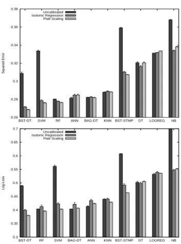
Figure 8. Performance of learning algorithms

each model with Isotonic Regression and Platt Scaling. Models are trained on 4k samples and calibrated on inde-pendent 1k samples. For each data set, learning algorithm, and calibration method, we select the model with the best performance using the same 1k points used for calibration, and report it’s performance on the large final test set. Figure 8 shows the squared error (top) and log-loss (bot-tom) for each learning method before and after calibra-tion. Each bar averages over five trials on each of the eight problems. Error bars representing 1 standard deviation for the means are shown. The probabilities predicted by four learning methods — boosted trees, SVMs, boosted stumps, and naive bayes — are dramatically improved by calibra-tion. Calibration does not help bagged tress, and actually hurts neural nets. Before calibration, the best models are random forests, bagged trees, and neural nets. After cali-bration, however, boosted trees, random forests, and SVMs predict the best probabilities.

7. Conclusions

In this paper we examined the probabilities predicted by ten different learning methods. Maximum margin meth-ods such as boosting and SVMs yield characteristic dis-tortions in their predictions. Other methods such as naive

bayes make predictions with the opposite distortion. And methods such as neural nets and bagged trees predict well-calibrated probabilities. We examined the effectiveness of Platt Scaling and Isotonic Regression for calibrating the predictions made by different learning methods. Platt Scal-ing is most effective when the data is small, but Isotonic Regression is more powerful when there is sufficient data to prevent overfitting. After calibration, the models that pre-dict the best probabilities are boosted trees, random forests, SVMs, uncalibrated bagged trees and uncalibrated neural nets.

ACKNOWLEDGMENTS

Thanks to B. Zadrozny and C. Elkan for the Isotonic Re-gression code, C. Young et al. at Stanford Linear Acceler-ator for the SLAC data, and A. Gualtieri at Goddard Space Center for help with the Indian Pines Data. This work was supported by NSF Award 0412930.

References

Ayer, M., Brunk, H., Ewing, G., Reid, W., & Silverman, E. (1955). An empirical distribution function for sampling with incomplete information. Annals of Mathematical Statistics, 5, 641–647.

Blake, C., & Merz, C. (1998). UCI repository of machine learning databases.

DeGroot, M., & Fienberg, S. (1982). The comparison and evaluation of forecasters. Statistician, 32, 12–22. Gualtieri, A., Chettri, S. R., Cromp, R., & Johnson, L.

(1999). Support vector machine classifiers as applied to aviris data. Proc. Eighth JPL Airborne Geoscience Workshop.

Niculescu-Mizil, A., & Caruana, R. (2005). Obtaining cal-ibrated probabilities from boosting. Proc. 21th Confer-ence on Uncertainty in Artificial IntelligConfer-ence (UAI ’05). AUAI Press.

Platt, J. (1999). Probabilistic outputs for support vector ma-chines and comparison to regularized likelihood meth-ods. Advances in Large Margin Classifiers (pp. 61–74). Robertson, T., Wright, F., & Dykstra, R. (1988). Order

restricted statistical inference. New York: John Wiley and Sons.

Zadrozny, B., & Elkan, C. (2001). Obtaining calibrated probability estimates from decision trees and naive bayesian classifiers. ICML (pp. 609–616).

Zadrozny, B., & Elkan, C. (2002). Transforming classi-fier scores into accurate multiclass probability estimates. KDD (pp. 694–699).