Elliptic Modular Forms and Their Applications

Don Zagier

Max-Planck-Institut für Mathematik, Vivatsgasse 7, 53111 Bonn, Germany E-mail: [email protected]

Foreword

These notes give a brief introduction to a number of topics in the classical theory of modular forms. Some of theses topics are (planned) to be treated in much more detail in a book, currently in preparation, based on various courses held at the Collège de France in the years 2000–2004. Here each topic is treated with the minimum of detail needed to convey the main idea, and longer proofs are omitted.

Classical (or “elliptic”) modular forms are functions in the complex upper half-plane which transform in a certain way under the action of a discrete subgroupΓ of SL(2,R)such as SL(2,Z). From the point of view taken here, there are two cardinal points about them which explain why we are interested. First of all, the space of modular forms of a given weight onΓ is finite dimen-sional and algorithmically computable, so that it is a mechanical procedure to prove any given identity among modular forms. Secondly, modular forms occur naturally in connection with problems arising in many other areas of mathematics. Together, these two facts imply that modular forms have a huge number of applications in other fields. The principal aim of these notes – as also of the notes on Hilbert modular forms by Bruinier and on Siegel modular forms by van der Geer – is to give a feel for some of these applications, rather than emphasizing only the theory. For this reason, we have tried to give as many and as varied examples of interesting applications as possible. These applications are placed in separate mini-subsections following the relevant sections of the main text, and identified both in the text and in the table of contents by the symbol♠. (The end of such a mini-subsection is correspond-ingly indicated by the symbol♥: these aremajor applications.) The subjects they cover range from questions of pure number theory and combinatorics to differential equations, geometry, and mathematical physics.

The notes are organized as follows. Section 1 gives a basic introduction to the theory of modular forms, concentrating on the full modular group

Γ₁ = SL(2,Z). Much of what is presented there can be found in standard textbooks and will be familiar to most readers, but we wanted to make the exposition self-contained. The next two sections describe two of the most im-portant constructions of modular forms, Eisenstein series and theta series. Here too most of the material is quite standard, but we also include a number of concrete examples and applications which may be less well known. Sec-tion 4 gives a brief account of Hecke theory and of the modular forms arising from algebraic number theory or algebraic geometry whoseL-series have Eu-ler products. In the last two sections we turn to topics which, although also classical, are somewhat more specialized; here there is less emphasis on proofs and more on applications. Section 5 treats the aspects of the theory con-nected with differentiation of modular forms, and in particular the differential equations which these functions satisfy. This is perhaps the most important single source of applications of the theory of modular forms, ranging from irrationality and transcendence proofs to the power series arising in mirror symmetry. Section 6 treats the theory of complex multiplication. This too is a classical theory, going back to the turn of the (previous) century, but we try to emphasize aspects that are more recent and less familiar: formulas for the norms and traces of the values of modular functions at CM points, Borcherds products, and explicit Taylor expansions of modular forms. (The last topic is particularly pretty and has applications to quite varied problems of num-ber theory.) A planned seventh section would have treated the integrals, or “periods,” of modular forms, which have a rich combinatorial structure and many applications, but had to be abandoned for reasons of space and time. Apart from the first two, the sections are largely independent of one another and can be read in any order. The text contains 29 numbered “Propositions” whose proofs are given or sketched and 20 unnumbered “Theorems” which are results quoted from the literature whose proofs are too difficult (in many cases,muchtoo difficult) to be given here, though in many cases we have tried to indicate what the main ingredients are. To avoid breaking the flow of the exposition, references and suggestions for further reading have not been given within the main text but collected into a single section at the end. Notations are standard (e.g.,Z,Q,RandCfor the integers, rationals, reals and complex numbers, respectively, andNfor the strictly positive integers). Multiplication precedes division hierarchically, so that, for instance,1/4πmeans1/(4π)and not(1/4)π.

The presentation in Sections 1–5 is based partly on notes taken by Chris-tian Grundh, Magnus Dehli Vigeland and my wife, Silke Wimmer-Zagier, of the lectures which I gave at Nordfjordeid, while that of Section 6 is partly based on the notes taken by John Voight of an earlier course on complex multiplication which I gave in Berekeley in 1992. I would like to thank all of them here, but especially Silke, who read each section of the notes as it was written and made innumerable useful suggestions concerning the exposition. And of course special thanks to Kristian Ranestad for the wonderful week in Nordfjordeid which he organized.

1 Basic Definitions

In this section we introduce the basic objects of study – the group SL(2,R)

and its action on the upper half plane, the modular group, and holomorphic modular forms – and show that the space of modular forms of any weight and level is finite-dimensional. This is the key to the later applications.

1.1 Modular Groups, Modular Functions and Modular Forms The upper half plane, denoted _H, is the set of all complex numbers with positive imaginary part:

H = z∈C|_I(z)>0.

The special linear group SL(2,R) acts on _Hin the standard way byMöbius transformations(or fractional linear transformations):

γ =

a b c d

: _H→_H, z→γz = γ(z) = az+b cz+d.

To see that this action is well-defined, we note that the denominator is non-zero and thatHis mapped toHbecause, as a sinple calculation shows,

I(γz) = I(z)

|cz+d|2. (1)

The transitivity of the action also follows by direct calculations, or alterna-tively we can viewHas the set of classes ofω1

ω2

∈C2_|ω

2= 0,I(ω1/ω2)>0

under the equivalence relation of multiplication by a non-zero scalar, in which case the action is given by ordinary matrix multiplication from the left. Notice that the matrices ±γ act in the same way on_H, so we can, and often will, work instead with the group PSL(2,R) =SL(2,R)/{±1}.

Elliptic modular functions and modular forms are functions in _H which are either invariant or transform in a specific way under the action of a dis-crete subgroup Γ of SL(2,R). In these introductory notes we will consider only the group Γ₁ =SL(2,Z) (the “full modular group”) and its congruence subgroups (subgroups of finite index ofΓ₁which are described by congruence conditions on the entries of the matrices). We should mention, however, that there are other interesting discrete subgroups of SL(2,R), most notably the non-congruence subgroups of SL(2,Z), whose corresponding modular forms have rather different arithmetic properties from those on the congruence sub-groups, and subgroups related to quaternion algebras over Q, which have a compact fundamental domain. The latter are important in the study of both Hilbert and Siegel modular forms, treated in the other contributions in this volume.

The modular group takes its name from the fact that the points of the quotient space Γ₁\Hare moduli (=parameters) for the isomorphism classes of elliptic curves over C. To each point z ∈ Hone can associate the lattice

Λz =Z.z + Z.1⊂Cand the quotient spaceEz =C/Λz, which is an elliptic curve, i.e., it is at the same time a complex curve and an abelian group. Conversely, every elliptic curve overC can be obtained in this way, but not uniquely: if E is such a curve, then E can be written as the quotientC/Λ

for some lattice (discrete rank 2 subgroup) Λ ⊂ C which is unique up to “homotheties”Λ→λΛwithλ∈C∗, and if we choose an oriented basis(ω₁, ω₂)

ofΛ(one withI(ω₁/ω₂)>0) and useλ=ω₂−1for the homothety, then we see thatE ∼=Ez for somez∈H, but choosing a different oriented basis replaces

zbyγzfor someγ∈Γ₁. The quotient spaceΓ₁\His the simplest example of what is called amoduli space, i.e., an algebraic variety whose points classify isomorphism classes of other algebraic varieties of some fixed type. A complex-valued function on this space is called amodular functionand, by virtue of the above discussion, can be seen as any one of four equivalent objects: a function fromΓ₁\HtoC, a functionf :H→Csatisfying the transformation equation

f(γz) =f(z)for everyz∈Hand everyγ∈Γ₁, a function assigning to every elliptic curveEoverCa complex number depending only on the isomorphism type of E, or a function on lattices in C satisfying F(λΛ) = F(Λ) for all latticesΛ and allλ∈ C×, the equivalence between f and F being given in one direction byf(z) = F(Λz)and in the other by F(Λ) =f(ω1/ω2) where (ω₁, ω₂)is any oriented basis ofΛ. Generally the term “modular function”, on

Γ₁or some other discrete subgroupΓ ⊂SL(2,R), is used only for meromorphic modular functions, i.e., Γ-invariant meromorphic functions in H which are of exponential growth at infinity (i.e., f(x+iy) = O(eCy_{) as y → ∞ and}

f(x+iy) =O(eC/y_{)as y →0 for some C >0), this latter condition being} equivalent to the requirement that f extends to a meromorphic function on the compactified spaceΓ\Hobtained by adding finitely many “cusps” toΓ\H

(see below).

It turns out, however, that for the purposes of doing interesting arithmetic the modular functions are not enough and that one needs a more general class of functions called modular forms. The reason is that modular functions have to be allowed to be meromorphic, because there are no global holomorphic functions on a compact Riemann surface, whereas modular forms, which have a more flexible transformation behavior, are holomorphic functions (on_Hand, in a suitable sense, also at the cusps). Every modular function can be repre-sented as a quotient of two modular forms, and one can think of the modular functions and modular forms as in some sense the analogues of rational num-bers and integers, respectively. From the point of view of functions on lattices, modular forms are simply functionsΛ→F(Λ)which transform under homo-theties byF(λΛ) =λ−k_{F(Λ)rather than simply byF(λΛ) =F(Λ)as before,} wherekis a fixed integer called theweightof the modular form. If we translate this back into the language of functions onHviaf(z) =F(Λz)as before, then we see thatf is now required to satisfy the modular transformation property

f

az+b cz+d

= (cz+d)kf(z) (2)

for allz∈_Hand alla b c d

∈Γ₁; conversely, given a functionf :_H→C satis-fying (2), we can define a funcion on lattices, homogeneous of degree−kwith respect to homotheties, byF(Z.ω₁+Z.ω₂) =ω−₂kf(ω₁/ω₂). As with modular functions, there is a standard convention: when the word “modular form” (on some discrete subgroupΓ of SL(2,R)) is used with no further adjectives, one generally means “holomorphic modular form”, i.e., a function f onH satisfy-ing (2) for all a b

c d

∈ Γ which is holomorphic in H and of subexponential growth at infinity (i.e., f satisfies the same estimate as above, but now for all rather than some C > 0). This growth condition, which corresponds to holomorphy at the cusps in a sense which we do not explain now, implies that the growth at infinity is in fact polynomial; more precisely,f automatically satisfiesf(z) =O(1)asy→ ∞andf(x+iy) =O(y−k)as y→0. We denote byMk(Γ)the space of holomorphic modular forms of weightkonΓ. As we will see in detail forΓ =Γ₁, this space is finite-dimensional, effectively com-putable for allk, and zero fork <0, and the algebraM_∗(Γ) :=_kMk(Γ)of all modular forms on Γ is finitely generated overC.

If we specialize (2) to the matrix1 1 0 1

, which belongs toΓ₁, then we see that any modular form onΓ₁ satisfiesf(z+ 1) =f(z)for allz∈H, i.e., it is a periodic function of period 1. It is therefore a function of the quantitye2πiz_, traditionally denotedq; more precisely, we have theFourier development

f(z) = ∞

n=0

ane2πinz =

∞

n=0 anqn

z∈_H, q = e2πiz, (3) where the fact that only termsqn withn≥0 occur is a consequence of (and in the case ofΓ₁, in fact equivalent to) the growth conditions onf just given. It is this Fourier development which is responsible for the great importance of modular forms, because it turns out that there are many examples of modular forms f for which the Fourier coefficients an in (3) are numbers that are of interest in other domains of mathematics.

1.2 The Fundamental Domain of the Full Modular Group

In the rest of §1 we look in more detail at the modular group. Because Γ₁

contains the element −1 = −1 0_{0 −1} which fixes every point of H, we can also consider the action of the quotient groupΓ₁=Γ₁/{±1}=PSL(2,Z)⊂

PSL(2,R)onH. It is clear from (2) that a modular form of odd weight onΓ₁

(or on any subgroup of SL(2,R)containing−1) must vanish, so we can restrict our attention to evenk. But then the “automorphy factor” (cz+d)k _{in (2) is} unchanged when we replaceγ∈Γ₁by−γ, so that we can consider equation (2) forkeven anda b

c d

∈Γ₁. By a slight abuse of notation, we will use the same notation for an elementγofΓ₁ and its image±γ inΓ₁, and, forkeven, will not distinguish between the isomorphic spacesMk(Γ1)andMk(Γ1).

The groupΓ₁is generated by the two elementsT =1 1 0 1

andS=₋0 1_{1 0}, with the relationsS2= (ST)3= 1. The actions of SandT onHare given by

S : z→ −1/z , T : z→z+ 1.

Thereforef is a modular form of weightkonΓ₁precisely whenf is periodic with period1 and satisfies the single further functional equation

f−1/z = zkf(z) (z∈H). (4)

If we know the value of a modular formf on some groupΓ at one point

z∈H, then equation (2) tells us the value at all points in the sameΓ₁-orbit asz. So to be able to completely determinef it is enough to know the value at one point from each orbit. This leads to the concept of afundamental domain forΓ, namely an open subsetF ⊂ Hsuch that no two distinct points of F are equivalent under the action ofΓ and every pointz∈HisΓ-equivalent to some point in the closureF of F.

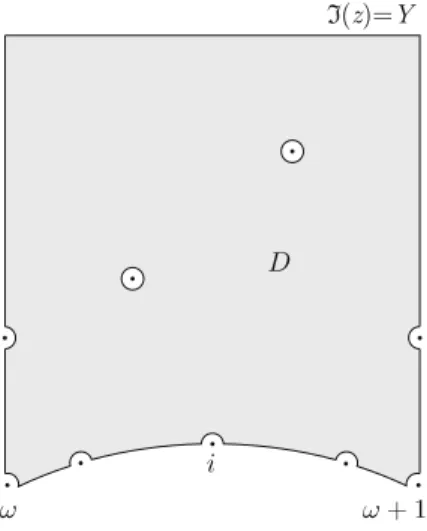
Proposition 1.The set F1 =

z∈H | |z|>1, |(z)| < 1₂

is a fundamental domain for the full modular groupΓ₁.(See Fig. 1A.)

Proof. Take a point z ∈ H. Then {mz+n | m, n ∈ Z} is a lattice in C. Every lattice has a point different from the origin of minimal modulus. Let

cz+dbe such a point. The integers c, dmust be relatively prime (otherwise we could dividecz+dby an integer to get a new point in the lattice of even smaller modulus). So there are integersaandbsuch thatγ₁=a b

c d

∈Γ₁. By the transformation property (1) for the imaginary party=I(z)we get that I(γ₁z)is a maximal member of{I(γz)|γ∈Γ₁}. Setz∗=Tnγ₁z=γ₁z +n,

where n is such that |(z∗)| ≤ ₂1. We cannot have |z∗| < 1, because then we would have I(−1/z∗) = I(z∗)/|z∗|2 > I(z∗) by (1), contradicting the maximality ofI(z∗). Soz∗∈ F₁, and zis equivalent under Γ₁to z∗.

Now suppose that we had twoΓ₁-equivalent pointsz₁andz₂=γz₁inF₁, with γ = ±1. This γ cannot be of the formTn _{since this would contradict} the condition |(z₁)|, |(z₂)| < 1

2, so γ =

_{a b}

c d

with c = 0. Note that I(z)>√3/2 for allz∈ F₁. Hence from (1) we get

√

3

2 < I(z2) =

I(z₁)

|cz₁+d|2 ≤

I(z₁) c2_I(z

1)2 < 2

c2√₃,

which can only be satisfied if c = ±1. Without loss of generality we may assume thatIz₁≤Iz₂. But|±z₁+d| ≥ |z₁|>1, and this gives a contradiction with the transformation property (1).

Remarks. 1. The points on the borders of the fundamental region are Γ₁ -equivalent as follows: First, the points on the two lines(z) =±1₂ are equiva-lent by the action ofT :z→z+ 1. Secondly, the points on the left and right halves of the arc|z|= 1are equivalent under the action of S:z→ −1/z. In fact, these are the only equivalences for the points on the boundary. For this reason we defineF₁to be the semi-closure ofF₁where we have added only the boundary points with non-positive real part (see Fig. 1B). Then every point ofHisΓ₁-equivalent to aunique point of F₁, i.e.,F₁ is astrict fundamental domain for the action of Γ₁. (But terminology varies, and many people use the words “fundamental domain” for the strict fundamental domain or for its closure, rather than for the interior.)

2. The description of the fundamental domain F₁ also implies the above-mentioned fact thatΓ₁ (orΓ₁) is generated byS andT. Indeed, by the very definition of a fundamental domain we know thatF₁and its translatesγF₁by elementsγ of Γ₁ cover _H, disjointly except for their overlapping boundaries (a so-called “tesselation” of the upper half-plane). The neighbors of F₁ are

T−1F₁, SF₁ and TF₁ (see Fig. 1C), so one passes from any translate γF₁

ofF₁ to one of its three neighbors by applying γSγ−1 orγT±1γ−1. In parti-cular, if the elementγ describing the passage fromF₁ to a given translated fundamental domainF₁ = γF₁ can be written as a word in S and T, then so can the element of Γ₁ which describes the motion from F₁ to any of the neighbors of F₁. Therefore by moving from neighbor to neighbor across the whole upper half-plane we see inductively that this property holds for every

γ∈Γ₁, as asserted. More generally, one sees that if one has given a fundamen-tal domainF for any discrete groupΓ, then the elements ofΓ which identify in pairs the sides ofF always generateΓ.

♠ Finiteness of Class Numbers

Let D be a negative discriminant, i.e., a negative integer which is congruent to 0 or 1 modulo 4. We consider binary quadratic forms of the formQ(x, y) =

Ax2+Bxy+Cy2 with A, B, C ∈ Z and B2−4AC = D. Such a form is definite (i.e.,Q(x, y)= 0for non-zero(x, y)∈R2) and hence has a fixed sign, which we take to be positive. (This is equivalent toA >0.) We also assume that Q is primitive, i.e., that gcd(A, B, C) = 1. Denote by QD the set of these forms. The groupΓ₁ (or indeed Γ₁) acts on _QD byQ→Q◦γ, where

(Q◦γ)(x, y) =Q(ax+by, cx+dy)forγ=±a b c d

∈Γ₁. We claim that the number of equivalence classes under this action is finite. This number, called theclass number of D and denoted h(D), also has an interpretation as the number of ideal classes (either for the ring of integers or, ifDis a non-trivial square multiple of some other discriminant, for a non-maximal order) in the imaginary quadratic fieldQ(√D), so this claim is a special case – historically the first one, treated in detail in Gauss’s Disquisitiones Arithmeticae – of the general theorem that the number of ideal classes in any number field is finite. To prove it, we observe that we can associate to any Q ∈ QD the unique rootzQ = (−B+√D)/2AofQ(z,1) = 0in the upper half-plane (here √

D = +i|D| by definition and A > 0 by assumption). One checks easily that _zQ◦γ = γ−1(zQ) for any γ ∈ Γ1, so each Γ1-equivalence class of forms Q∈_QD has a unique representative belonging to the set

QredD =

[A, B, C]∈_QD | −A < B ≤A < C or 0≤B≤A = C

(5) of Q ∈ _QD for which _zQ ∈ F₁ (the so-called reduced quadratic forms of discriminant D), and this set is finite because C ≥ A ≥ |B| implies |D| = 4AC−B2 _≥3A2_{, so that both A and B are bounded in absolute value by}

|D|/3, after whichCis fixed byC= (B2_{−D)/4A. This even gives us a way}

to compute h(D) effectively, e.g., Qred₋₄₇ = {[1,1,12], [2,±1,6], [3,±1,4]}

and hence h(−47) = 5. We remark that the class numbersh(D), or a small modification of them, are themselves the coefficients of a modular form (of weight 3/2), but this will not be discussed further in these notes. ♥

1.3 The Finite Dimensionality ofM_k(Γ)

We end this section by applying the description of the fundamental domain to show that Mk(Γ1) is finite-dimensional for every k and to get an upper

bound for its dimension. In §2 we will see that this upper bound is in fact the correct value.

If f is a modular form of weight k onΓ₁ or any other discrete group Γ, then f is not a well-defined function on the quotient space Γ\H, but the transformation formula (2) implies that the order of vanishing ordz(f) at a pointz∈Hdepends only on the orbitΓ z. We can therefore define a local order of vanishing, ordP(f), for eachP ∈Γ\H. The key assertion is that the total number of zeros of f, i.e., the sum of all of these local orders, depends only onΓ and k. But to make this true, we have to look more carefully at the geometry of the quotient space Γ\H, taking into account the fact that some points (the so-called elliptic fixed points, corresponding to the points

z∈Hwhich have a non-trivial stabilizer for the image ofΓ in PSL(2,R)) are singular and also thatΓ\His not compact, but has to be compactified by the addition of one or more further points calledcusps. We explain this for the caseΓ =Γ₁.

In §1.2 we identified the quotient space Γ₁\H as a set with the semi-closureF₁ ofF₁and as a topological space with the quotient ofF₁obtained by identifying the opposite sides (lines(z) =±1₂ or halves of the arc|z|= 1) of the boundary∂F₁. For a generic point ofF₁the stabilizer subgroup ofΓ₁

is trivial. But the two pointsω= 1₂(−1 +i√3) =e2πi/3 andi are stabilized by the cyclic subgroups of order 3 and 2 generated byST andSrespectively. This means that in the quotient manifoldΓ₁\H,ω andi are singular. (From a metric point of view, they have neighborhoods which are not discs, but quotients of a disc by these cyclic subgroups, with total angle120◦ or 180◦

instead of360◦.) If we define an integernP for everyP ∈Γ1\Has the order

of the stabilizer in Γ₁ of any point in _H representingP, then nP equals 2 or 3 if P is Γ₁-equivalent to i or ω and nP = 1 otherwise. We also have to consider the compactified quotientΓ₁\Hobtained by adding a point at infinity (“cusp”) toΓ₁\H. More precisely, forY >1the image inΓ₁\Hof the part ofH above the lineI(z) =Y can be identified via q =e2πiz _{with the punctured} disc0 < q < e−2πY_{. Equation (3) tells us that a holomorphic modular form} of any weight k onΓ₁ is not only a well-defined function on this punctured disc, but extends holomorphically to the point q = 0. We therefore define

Γ₁\H=Γ₁\H∪ {∞}, where the point “∞” corresponds to q = 0, withq as a local parameter. One can also think ofΓ₁\Has the quotient ofHbyΓ₁, where H=H∪Q∪{∞}is the space obtained by adding the fullΓ₁-orbitQ∪{∞}of ∞to_H. We define theorder of vanishing at infinity off, denoted ord_∞(f), as the smallest integernsuch thatan = 0in the Fourier expansion (3). Proposition 2.Let f be a non-zero modular form of weight kon Γ₁. Then

P_∈Γ_1\H

1 nP

ordP(f) + ord∞(f) =

k

12. (6)

Proof. LetDbe the closed set obtained fromF₁by deletingε-neighborhoods of all zeros off and also the “neighborhood of infinity”_I(z)> Y =ε−1, where

εis chosen sufficiently small that all of these neighborhoods are disjoint (see Fig. 2.) Sincef has no zeros inD, Cauchy’s theorem implies that the integral of dlogf(z)= f

_(z)

f(z) dz over the boundary ofDis 0. This boundary consists

of several parts: the horizontal line from−1₂+iY to 1₂+iY, the two vertical lines fromωto−1₂+iY and fromω+ 1to 1₂+iY (with someε-neighborhoods removed), the arc of the circle |z| = 1 from ω to ω + 1 (again with some

ε-neighborhoods deleted), and the boundaries of the ε-neighborhoods of the zerosP off. These latter have total angle2πifP is not an elliptic fixed point

Fig. 2. The zeros of a modular form

(they consist of a full circle ifPis an interior point ofF₁and of two half-circles ifP corresponds to a boundary point ofF₁different fromω,ω+ 1ori), and total angle πor 2π/3 ifP ∼ior ω. The corresponding contributions to the integral are as follows. The two vertical lines together give 0, becausef takes on the same value on both and the orientations are opposite. The horizontal line from−1

2+iY to 1

2+iY gives a contribution 2πiord∞(f), because d(logf)

is the sum of ord_∞(f)dq/q and a function of q which is holomorphic at 0, and this integral corresponds to an integral around a small circle|q|=e−2πY aroundq= 0. The integral on the boundary of the deletedε-neighborhood of a zeroP off contributes2πiordP(f)ifnP = 1by Cauchy’s theorem, because ordP(f) is the residue of d(logf(z)) at z = P, while for nP > 1 we must divide bynP because we are only integrating over one-half or one-third of the full circle around P. Finally, the integral along the bottom arc contributes

πik/6, as we see by breaking up this arc into its left and right halves and applying the formula dlogf(Sz) =dlogf(z) +kdz/z, which is a consequence of the transformation equation (4). Combining all of these terms with the appropriate signs dictated by the orientation, we obtain (6). The details are left to the reader.

Corollary 1.The dimension of Mk(Γ1) is 0 for k < 0 or k odd, while for

evenk≥0 we have

dimMk(Γ1) ≤

[k/12] + 1 ifk≡2 (mod 12)

[k/12] ifk≡2 (mod 12). (7)

Proof. Let m = [k/12] + 1 and choose m distinct non-elliptic points Pi ∈

combinationf of them which vanishes in allPi, by linear algebra. But then

f ≡0 by the proposition, sincem > k/12, so the fi are linearly dependent. HencedimMk(Γ1)≤m. Ifk≡2 (mod 12)we can improve the estimate by 1

by noticing that the only way to satisfy (6) is to have (at least) a simple zero ati and a double zero atω (contributing a total of 1/2 + 2/3 = 7/6to

ordP(f)/nP) together with k/12−7/6 =m−1further zeros, so that the same argument now givesdimMk(Γ1)≤m−1.

Corollary 2.The space M₁₂(Γ₁) has dimension ≤2, and iff, g ∈M₁₂(Γ₁)

are linearly independent, then the mapz →f(z)/g(z)gives an isomorphism from Γ₁\H∪ {∞} toP1_(C).

Proof. The first statement is a special case of Corollary 1. Suppose that f

andg are linearly independent elements ofM₁₂(Γ₁). For any(0,0)= (λ, μ)∈

C2_{the modular formλf−μgof weight 12 has exactly one zero inΓ}

1\H∪{∞}

by Proposition 2, so the modular function ψ = f /g takes on every value

(μ:λ)∈P1_{(C)exactly once, as claimed.}

We will make an explicit choice off,gandψin §2.4, after we have introduced the “discriminant function” Δ(z)∈M₁₂(Γ₁).

The true interpretation of the factor 1/12 multiplying k in equation (6) is as 1/4π times the volume of Γ₁\H, taken with respect to the hyperbolic metric. We say only a few words about this, since these ideas will not be used again. To give a metric on a manifold is to specify the distance be-tween any two sufficiently near points. Thehyperbolic metric in _His defined by saying that the hyperbolic distance between two points in a small neigh-borhood of a point z =x+iy ∈ H is very nearly 1/y times the Euclidean distance between them, so the volume element, which in Euclidean geometry is given by the 2-formdx dy, is given in hyperbolic geometry bydμ=y−2dx dy. Thus

VolΓ₁\H) =

F1

dμ =

1/2 −1/2

_∞

√ 1−x2

dy y2

dx

=

₁/2 −1/2

dx

√

1−x2 = arcsin(x)

1/2

−1/2 = π

3.

Now we can consider other discrete subgroups of SL(2,R)which have a fun-damental domain of finite volume. (Such groups are usually calledFuchsian groups of the first kind, and sometimes “lattices”, but we will reserve this lat-ter lat-term for discrete cocompact subgroups of Euclidean spaces.) Examples are the subgroupsΓ ⊂Γ₁ of finite index, for which the volume ofΓ\Hisπ/3

times the index ofΓ inΓ₁(or more precisely, of the image ofΓ in PSL(2,R)

in Γ₁). If Γ is any such group, then essentially the same proof as for Pro-position 2 shows that the number of Γ-inequivalent zeros of any non-zero

modular form f ∈ Mk(Γ) equals kVol(Γ\H)/4π, where just as in the case of Γ₁ we must count the zeros at elliptic fixed points or cusps of Γ with appropriate multiplicities. The same argument as for Corollary 1 of Propos-ition 2 then tells usMk(Γ)is finite dimensional and gives an explicit upper bound:

Proposition 3.LetΓ be a discrete subgroup of SL(2,R)for which Γ\H has finite volumeV. Then dimMk(Γ)≤

kV

4π + 1 for allk∈Z.

In particular, we have Mk(Γ) ={0} for k < 0 and M0(Γ) = C, i.e., there

are no holomorphic modular forms of negative weight on any groupΓ, and the only modular forms of weight 0 are the constants. A further consequence is that any three modular forms onΓ are algebraically dependent. (Iff, g, h

were algebraically independent modular forms of positive weights, then for largekthe dimension of Mk(Γ)would be at least the number of monomials inf,g,hof total weightk, which is bigger than some positive multiple ofk2, contradicting the dimension estimate given in the proposition.) Equivalent-ly, any two modular functions onΓ are algebraically dependent, since every modular function is a quotient of two modular forms. This is a special case of the general fact that there cannot be more than nalgebraically indepen-dent algebraic functions on an algebraic variety of dimensionn. But the most important consequence of Proposition 3 from our point of view is that it is the origin of the (unreasonable?) effectiveness of modular forms in number theory: if we have two interesting arithmetic sequences{an}n_≥0and{bn}n_≥0

and conjecture that they are identical (and clearly many results of number theory can be formulated in this way), then if we can show that bothanqn andbnqn are modular forms of the same weight and group, we need only verify the equalityan =bn for a finite number ofn in order to know that it is true in general. There will be many applications of this principle in these notes.

2 First Examples: Eisenstein Series

and the Discriminant Function

In this section we construct our first examples of modular forms: the Eisenstein seriesEk(z)of weightk >2and the discriminant functionΔ(z)of weight 12, whose definition is closely connected to the non-modular Eisenstein series

E₂(z).

2.1 Eisenstein Series and the Ring Structure of M_∗(Γ₁)

There are two natural ways to introduce the Eisenstein series. For the first, we observe that the characteristic transformation equation (2) of a modular

form can be written in the formf|kγ=f forγ ∈Γ, wheref|kγ :H→C is defined by

f_kg(z) = (cz+d)−kf

az+b cz+d

z∈C, g =

a b c d

∈SL(2,R).

(8) One checks easily that for fixedk∈Z, the mapf →f|kgdefines an operation of the group SL(2,R)(i.e., f|k(g₁g₂) = (f|kg₁)|kg₂ for all g₁, g₂∈ SL(2,R)) on the vector space of holomorphic functions in _H having subexponential or polynomial growth. The space Mk(Γ) of holomorphic modular forms of weightk on a groupΓ ⊂SL(2,R)is then simply the subspace of this vector space fixed byΓ.

If we have a linear actionv→v|gof afinitegroupGon a vector spaceV, then an obvious way to construct a G-invariant vector in V is to start with an arbitrary vector v₀ ∈ V and form the sumv =_g∈Gv₀|g (and to hope that the result is non-zero). If the vector v₀ is invariant under some sub-groupG₀⊂G, then the vector v₀|g depends only on the coset G₀g∈G₀\G

and we can form instead the smaller sumv =_g∈G

0\Gv0|g, which again is G-invariant. IfGis infinite, the same method sometimes applies, but we now have to be careful about convergence. If the vectorv₀ is fixed by an infinite subgroupG₀ofG, then this improves our chances because the sum overG₀\G

is much smaller than a sum over all ofG (and in any case_g∈Gv|g has no chance of converging since every term occurs infinitely often). In the context when G = Γ ⊂ SL(2,R) is a Fuchsian group (acting by |k) and v₀ a ra-tional function, the modular forms obtained in this way are called Poincaré series. An especially easy case is that when v₀ is the constant function “1” and Γ₀ = Γ_∞, the stabilizer of the cusp at infinity. In this case the series

Γ∞\Γ1|kγis called anEisenstein series.

Let us look at this series more carefully whenΓ =Γ₁. A matrixa b c d

∈ SL(2,R)sends∞toa/c, and hence belongs to the stabilizer of∞if and only ifc= 0. InΓ₁ these are the matrices±1n

0 1

withn∈Z, i.e., up to sign the matricesTn_{. We can assume thatkis even (since there are no modular forms} of odd weight onΓ₁) and hence work withΓ₁=PSL(2,Z), in which case the stabilizer Γ_∞ is the infinite cyclic group generated byT. If we multiply an arbitrary matrixγ=a b

c d

on the left by1n

0 1

, then the resulting matrixγ=

_{a+nc b+nd}

c d

has the same bottom row asγ. Conversely, ifγ=ab c d

∈Γ₁has the same bottom row asγ, then from(a−a)d−(b−b)c= det(γ)−det(γ) = 0

and(c, d) = 1(the elements of any row or column of a matrix in SL(2,Z)are coprime!) we see thata−a=nc,b−b=ndfor somen∈Z, i.e.,γ=Tn_γ. Since every coprime pair of integers occurs as the bottom row of a matrix in SL(2,Z), these considerations give the formula

Ek(z) =

γ∈Γ∞\Γ1

1_kγ =

γ∈Γ∞\Γ1

1_kγ = 1 2

c, d∈Z

(c,d) = 1 1

for the Eisenstein series (the factor 1₂ arises because (c d)and(−c −d)give the same element of Γ₁\Γ₁). It is easy to see that this sum is absolutely convergent fork >2 (the number of pairs (c, d)with N ≤ |cz+d|< N+ 1

is the number of lattice points in an annulus of areaπ(N + 1)2_−πN2 _and

hence is O(N), so the series is majorized by∞_N=1N1−k_{), and this absolute} convergence guarantees the modularity (and, since it is locally uniform inz, also the holomorphy) of the sum. The function Ek(z)is therefore a modular form of weightkfor all evenk≥4. It is also clear that it is non-zero, since for I(z)→ ∞all the terms in (9) except(c d) = (±1 0)tend to 0, the convergence of the series being sufficiently uniform that their sum also goes to 0 (left to the reader), soEk(z) = 1 +o(1)= 0.

The second natural way of introducing the Eisenstein series comes from the interpretation of modular forms given in the beginning of §1.1, where we identified solutions of the transformation equation (2) with functions on lat-tices Λ ⊂C satisfying the homogeneity condition F(λΛ) = λ−kF(Λ) under homothetiesΛ→λΛ. An obvious way to produce such a homogeneous func-tion – if the series converges – is to form the sumGk(Λ) =1₂

λ∈Λ0λ−

k _of the(−k)th powers of the non-zero elements ofΛ. (The factor “1

2” has again

been introduce to avoid counting the vectors λ and −λ doubly when k is even; if kis odd then the series vanishes anyway.) In terms of z ∈_Hand its associated latticeΛz=Z.z+Z.1, this becomes

Gk(z) =

1 2

m, n_∈Z

(m,n) =(0,0) 1

(mz+n)k (k >2, z∈H), (10)

where the sum is again absolutely and locally uniformly convergent fork >2, guaranteeing thatGk∈Mk(Γ1). The modularity can also be seen directly by

noting that(Gk|kγ)(z) =_m,n(mz+n)−k where (m, n) = (m, n)γ runs over the non-zero vectors ofZ2{(0,0)}as(m, n)does.

In fact, the two functions (9) and (10) are proportional, as is easily seen: any non-zero vector(m, n)∈Z2can be written uniquely asr(c, d)withr(the greatest common divisor ofmandn) a positive integer andcanddcoprime integers, so

Gk(z) = ζ(k)Ek(z), (11)

where ζ(k) = _r≥11/rk _{is the value atk of the Riemann zeta function. It} may therefore seem pointless to have introduced both definitions. But in fact, this is not the case. First of all, each definition gives a distinct point of view and has advantages in certain settings which are encountered at later points in the theory: theEk definition is better in contexts like the famous Rankin-Selberg method where one integrates the product of the Eisenstein series with another modular form over a fundamental domain, while theGk definition is better for analytic calculations and for the Fourier development given in §2.2.

Moreover, if one passes to other groups, then there areσEisenstein series of each type, whereσis the number of cusps, and, although they span the same vector space, they are not individually proportional. In fact, we will actually want to introduce athird normalization

Gk(z) =

(k−1)!

(2πi)k Gk(z) (12)

because, as we will see below, it has Fourier coefficients which are rational numbers (and even, with one exception, integers) and because it is a normal-ized eigenfunction for the Hecke operators discussed in §4.

As a first application, we can now determine the ring structure ofM_∗(Γ₁)

Proposition 4.The ringM_∗(Γ₁)is freely generated by the modular formsE₄

andE₆.

Corollary.The inequality (7)for the dimension ofMk(Γ1)is an equality for

all evenk≥0.

Proof. The essential point is to show that the modular forms E₄(z) and

E₆(z)are algebraically independent. To see this, we first note that the forms

E₄(z)3 _{and E}

6(z)2 of weight 12 cannot be proportional. Indeed, if we had E₆(z)2 = λE₄(z)3 for some (necessarily non-zero) constant λ, then the meromorphic modular form f(z) = E₆(z)/E₄(z) of weight 2 would satisfy

f2=λE₄(and alsof3=λ−1E₆) and would hence be holomorphic (a function whose square is holomorphic cannot have poles), contradicting the inequal-ity dimM₂(Γ₁) ≤ 0 of Corollary 1 of Proposition 2. But any two modular formsf₁andf₂of the same weight which are not proportional are necessarily algebraically independent. Indeed, if P(X, Y) is any polynomial in C[X, Y]

such that P(f₁(z), f₂(z)) ≡ 0, then by considering the weights we see that

Pd(f1, f2)has to vanish identically for each homogeneous componentPdofP. ButPd(f1, f2)/f2d =p(f1/f2)for some polynomial p(t) in one variable, and

sincephas only finitely many roots we can only havePd(f1, f2)≡0iff1/f2

is a constant. It follows thatE3

4 andE62, and hence alsoE4 andE6, are

alge-braically independent. But then an easy calculation shows that the dimension of the weightkpart of the subring ofM_∗(Γ₁)which they generate equals the right-hand side of the inequality (7), so that the proposition and corollary follow from this inequality.

2.2 Fourier Expansions of Eisenstein Series

Recall from (3) that any modular form onΓ₁ has a Fourier expansion of the form∞_n=0anqn, whereq=e2πiz. The coefficientsanoften contain interesting arithmetic information, and it is this that makes modular forms important for classical number theory. For the Eisenstein series, normalized by (12), the coefficients are given by:

Proposition 5.The Fourier expansion of the Eisenstein seriesGk(z) (keven,

k >2) is

Gk(z) = −

Bk

2k + ∞

n=1

σk−1(n)qn, (13)

whereBk is thekth Bernoulli number and where σk−1(n)for n∈Ndenotes the sum of the (k−1)st powers of the positive divisors of n.

We recall that the Bernoulli numbers are defined by the generating function

_∞

k=0Bkxk/k! =x/(ex−1)and that the first values ofBk (k >0 even) are given by B₂ = 1₆, B₄ =−₃₀1, B₆ = ₄₂1, B₈ =−₃₀1, B₁₀ = ₆₆5,B₁₂ =−₂₇₃₀691, andB₁₄= 7₆.

Proof. A well known and easily proved identity of Euler states that

n∈Z

1 z+n =

π tanπz

z∈C\Z, (14)

where the sum on the left, which is not absolutely convergent, is to be inter-preted as a Cauchy principal value (= limN_−M whereM, N tend to infinity withM−N bounded). The function on the right is periodic of period 1 and its Fourier expansion forz∈His given by

π

tanπz = π cosπz sinπz = πi

eπiz_+e−πiz

eπiz_−e−πiz = −πi

1 +q

1−q = −2πi

1 2+ ∞ r=1 qr ,

whereq=e2πiz_{. Substitute this into (14), differentiatek−1times and divide} by(−1)k−1_{(k−1)! to get}

n_∈Z

1 (z+n)k =

(−1)k−1

(k−1)! dk−1

dzk₋₁

π tanπz

=(−2πi)

k

(k−1)! ∞

r=1 rk−1qr (k≥2, z∈H),

an identity known as Lipschitz’s formula. Now the Fourier expansion of Gk (k >2even) is obtained immediately by splitting up the sum in (10) into the terms withm= 0and those withm= 0:

Gk(z) =

1 2

n_∈Z n =0

1 nk +

1 2

m, n_∈Z m ₌₀

1

(mz+n)k =

∞

n=1 1 nk +

∞

m=1 ∞

n=−∞

1 (mz+n)k

= ζ(k) + (2πi)

k

(k−1)! ∞

m=1 ∞

r=1

rk−1qmr

= (2πi)

k

(k−1)!

−Bk

2k + ∞

n=1

σk₋₁(n)qn

,

where in the last line we have used Euler’s evaluation ofζ(k)(k >0 even) in terms of Bernoulli numbers. The result follows.

The first three examples of Proposition 5 are the expansions G4(z) =

1

240 + q + 9q

2 _{+ 28q}3 _{+ 73q}4 _{+ 126q}5 _{+ 252q}6 _{+· · · ,}

G6(z) = − 1

504 + q + 33q

2 _{+ 244q}3 _{+ 1057q}4 _{+ · · · ,}

G8(z) = 1

480 + q + 129q

2 _{+ 2188q}3 _{+ · · · .}

The other two normalizations of these functions are given by

G₄(z) =16π 4

3! G4(z) = π4

90E4(z), E4(z) = 1 + 240q + 2160q

2 _{+· · · ,} G₆(z) =−64π

6

5! G6(z) = π6

945E6(z), E6(z) = 1 − 504q − 16632q

2 _{− · · · ,} G₈(z) =256π

8

7! G8(z) = π8

9450E8(z), E8(z) = 1 + 480q+ 61920q

2 _{+· · · .}

Remark. We have discussed only Eisenstein series on the full modular group in detail, but there are also various kinds of Eisenstein series for subgroups

Γ ⊂ Γ₁. We give one example. Recall that a Dirichlet character modulo

N ∈Nis a homomorphismχ : (Z/NZ)∗ →C∗, extended to a mapχ:Z→C

(traditionally denoted by the same letter) by settingχ(n)equal toχ(nmodN)

if(n, N) = 1 and to 0 otherwise. Ifχ is a non-trivial Dirichlet character and

k a positive integer with χ(−1) = (−1)k, then there is an Eisenstein series having the Fourier expansion

Gk,χ(z) = ck(χ) +

∞

n=1 d|n

χ(d)dk−1

qn

which is a “modular form of weightkand characterχonΓ₀(N).” (This means that Gk,χ(azcz++db) = χ(a)(cz +d)

k_G

k,χ(z) for any z ∈ H and any

_{a b}

c d

∈ SL(2,Z)with c ≡0 (mod N).) Here ck(χ)∈Qis a suitable constant, given explicitly byck(χ) = 1₂L(1−k, χ), whereL(s, χ)is the analytic continuation of the Dirichlet series∞_n=1χ(n)n−s_.

The simplest example, for N = 4 and χ = χ₋₄ the Dirichlet character modulo 4 given by

χ₋₄(n) =

⎧ ⎪ ⎨ ⎪ ⎩

+1 ifn≡1 (mod 4), −1 ifn≡3 (mod 4),

0 ifnis even

(15)

and k= 1, is the series

G1,χ₋₄(z) =c1(χ−4) + ∞

n=1

⎛ ⎝

d|n

χ₋₄(d)

⎞ ⎠qn =1

4+q+q

2_+q4_{+ 2q}5_+q8_{+· · · .}

(The fact that L(0, χ₋₄) = 2c₁(χ₋₄) = 1

2 is equivalent via the functional

equation ofL(s, χ₋₄)to Leibnitz’s famous formula L(1, χ₋₄) = 1−1 3 +

1 5−

· · ·= π

4.) We will see this function again in §3.1.

♠ Identities Involving Sums of Powers of Divisors

We now have our first explicit examples of modular forms and their Fourier expansions and can immediately deduce non-trivial number-theoretic identi-ties. For instance, each of the spacesM₄(Γ₁),M₆(Γ₁),M₈(Γ₁),M₁₀(Γ₁)and

M₁₄(Γ₁) has dimension exactly 1 by the corollary to Proposition 2, and is therefore spanned by the Eisenstein seriesEk(z)with leading coefficient 1, so we immediately get the identities

E₄(z)2 = E₈(z), E₄(z)E₆(z) = E₁₀(z), E₆(z)E₈(z) = E₄(z)E₁₀(z) = E₁₄(z).

Each of these can be combined with the Fourier expansion given in Proposit-ion 5 to give an identity involving the sums-of-powers-of-divisors functProposit-ions

σk₋₁(n), the first and the last of these being n₋₁

m=1

σ₃(m)σ₃(n−m) = σ7(n)−σ3(n)

120 ,

n−1 m=1

σ₃(m)σ₉(n−m) = σ13(n)−11σ9(n) + 10σ3(n)

2640 .

Of course similar identities can be obtained from modular forms in higher weights, even though the dimension ofMk(Γ1) is no longer equal to 1. For

instance, the fact thatM₁₂(Γ₁)is 2-dimensional and contains the three modu-lar forms E₄E₈, E₆2 and E₁₂ implies that the three functions are linearly dependent, and by looking at the first two terms of the Fourier expansions we find that the relation between them is given by441E₄E₈+ 250E₆2= 691E₁₂, a formula which the reader can write out explicitly as an identity among sums-of-powers-of-divisors functions if he or she is so inclined. It is not easy to obtain any of these identities by direct number-theoretical reasoning (although in fact it can be done). ♥

2.3 The Eisenstein Series of Weight2

In §2.1 and §2.2 we restricted ourselves to the case when k > 2, since then the series (9) and (10) are absolutely convergent and therefore define modular forms of weightk. But the final formula (13) for the Fourier expansion ofGk(z) converges rapidly and defines a holomorphic function ofz also fork = 2, so

in this weight we can simply define the Eisenstein series G₂, G₂ and E₂ by equations (13), (12), and (11), respectively, i.e.,

G2(z) = − 1 24 +

∞

n=1

σ₁(n)qn = −1

24+q+ 3q

2_{+ 4q}3_{+ 7q}4_{+ 6q}5_{+· · · ,}

G₂(z) = −4π2G₂(z), E₂(z) = 6

π2G2(z) = 1 − 24q −72q

2 _{− · · · .}

(17) Moreover, the same proof as for Proposition 5 still shows thatG₂(z)is given by the expression (10), if we agree to carry out the summation over n first and then overm:

G₂(z) = 1 2

n =0

1 n2 +

1 2

m =0n∈Z

1

(mz+n)2. (18)

The only difference is that, because of the non-absolute convergence of the double series, we can no longer interchange the order of summation to get the modular transformation equation G₂(−1/z) = z2_G

2(z). (The equation G₂(z+ 1) =G₂(z), of course, still holds just as for higher weights.) Never-theless, the function G₂(z)and its multiples E₂(z)and G₂(z) do have some modular properties and, as we will see later, these are important for many applications.

Proposition 6.Forz∈Handa b c d

∈SL(2,Z)we have

G₂

az+b cz+d

= (cz+d)2G₂(z) −πic(cz+d). (19) Proof. There are many ways to prove this. We sketch one, due to Hecke, since the method is useful in many other situations. The series (10) for k = 2

does not converge absolutely, but it is just at the edge of convergence, since

m,n|mz+n|−

λ _{converges for any real number λ >2. We therefore modify} the sum slightly by introducing

G₂,ε(z) =

1 2

m, n

1

(mz+n)2|_mz+n|2ε (z∈H, ε >0). (20) (Here means that the value (m, n) = (0,0) is to be omitted from the summation.) The new series converges absolutely and transforms by

G₂,ε

_az+b

cz+d

= (cz +d)2_{|cz +d|}2ε_G

2,ε(z). We claim that lim

ε_→0G2,ε(z) exists and equals G₂(z)−π/2y, where y = _I(z). It follows that each of the three non-holomorphic functions

G∗₂(z) = G₂(z)− π 2y, E

∗

2(z) = E2(z)− 3 πy, G

∗

2(z) = G2(z) + 1 8πy

(21) transforms like a modular form of weight 2, and from this one easily deduces the transformation equation (19) and its analogues forE₂ andG₂. To prove

the claim, we define a functionIε by

Iε(z) =

_∞

−∞

dt (z+t)2_|z+t|2ε

z∈_H, ε >−1 2

.

Then forε >0we can write

G₂,ε−

∞

m=1

Iε(mz) =

∞

n=1 1 n2+2ε

+ ∞

m=1 ∞

n_=−∞

1

(mz+n)2|_mz+n|2ε −

n+1

n

dt

(mz+t)2|_mz+t|2ε

.

Both sums on the right converge absolutely and locally uniformly forε >−1 2

(the second one because the expression in square brackets is O|mz+n|−3−2ε by the mean-value theorem, which tells us that f(t)−f(n)for any differen-tiable function f is bounded in n ≤ t ≤ n+ 1 by maxn_≤u_≤n+1|f(u)|), so

the limit of the expression on the right asε→0 exists and can be obtained simply by puttingε= 0in each term, where it reduces to G₂(z)by (18). On the other hand, forε >−1₂ we have

Iε(x+iy) =

_∞

−∞

dt

(x+t+iy)2_((x+t)2_+y2₎ε

=

_∞

−∞

dt

(t+iy)2_(t2_+y2₎ε =

I(ε) y1+2ε, whereI(ε) =_−∞∞ (t+i)−2(t2₊₁₎−ε_{dt, so}∞

m=1Iε(mz) =I(ε)ζ(1+2ε)/y1+2ε forε >0. Finally, we haveI(0) = 0 (obvious),

I(0) = −

_∞

−∞

log(t2_{+ 1)} (t+i)2 dt =

1 + log(t2_{+ 1)}

t+i −tan

−1_t∞ −∞

= −π ,

andζ(1 + 2ε) = 1

2ε+O(1), so the productI(ε)ζ(1 + 2ε)/y

1+2ε_{tends to−π/2y} asε→0. The claim follows.

Remark.The transformation equation (18) says thatG₂is an example of what is called aquasimodular form, while the functions G∗₂, E₂∗ andG∗₂ defined in (21) are so-called almost holomorphic modular forms of weight 2. We will return to this topic in Section 5.

2.4 The Discriminant Function and Cusp Forms

Forz∈Hwe define thediscriminant function Δ(z)by the formula

Δ(z) = e2πiz ∞

n=1

(The name comes from the connection with the discriminant of the elliptic curveEz=C/(Z.z+Z.1), but we will not discuss this here.) Since|e2πiz|<1 forz∈H, the terms of the infinite product are all non-zero and tend exponen-tially rapidly to 1, so the product converges everywhere and defines a holomor-phic and everywhere non-zero function in the upper half-plane. This function turns out to be a modular form and plays a special role in the entire theory. Proposition 7.The functionΔ(z)is a modular form of weight12on SL(2,Z). Proof. SinceΔ(z)= 0, we can consider its logarithmic derivative. We find

1 2πi

d

dzlog Δ(z) = 1−24 ∞

n=1

n e2πinz

1−e2πinz = 1−24

∞

m=1

σ₁(m)e2πimz = E₂(z),

where the second equality follows by expanding e

2πinz

1−e2πinz as a geometric series∞_r=1e2πirnz_{and interchanging the order of summation, and the third} equality from the definition of E₂(z) in (17). Now from the transformation equation forE₂ (obtained by comparing (19) and(11)) we find

1 2πi

d dzlog

_Δaz+b cz+d

(cz+d)12_Δ(z)

= 1

(cz+d)2E2

az+b cz+d

− 12

2πi c

cz+d−E2(z) = 0.

In other words,(Δ|₁₂γ)(z) =C(γ) Δ(z) for allz ∈H and all γ ∈Γ₁, where

C(γ)is a non-zero complex number depending only onγ, and whereΔ|₁₂γ is defined as in (8). It remains to show thatC(γ) = 1for allγ. ButC:Γ₁→C∗

is a homomorphism because Δ → Δ|₁₂γ is a group action, so it suffices to check this for the generatorsT =1 1

0 1

and S = 0−1 1 0

of Γ₁. The first is obvious sinceΔ(z)is a power series in e2πiz _{and hence periodic of period 1,} while the second follows by substitutingz =iinto the equation Δ(−1/z) = C(S)z12Δ(z)and noting thatΔ(i)= 0.

Let us look at this functionΔ(z)more carefully. We know from Corollary 1 to Proposition 2 that the space M₁₂(Γ₁) has dimension at most 2, so Δ(z)

must be a linear combination of the two functions E₄(z)3 _andE

6(z)2. From

the Fourier expansionsE3

4 = 1 + 720q+· · ·, E6(z)2 = 1−1008q+· · · and Δ(z) =q+· · · we see that this relation is given by

Δ(z) = 1 1728

E₄(z)3 − E₆(z)2. (23) This identity permits us to give another, more explicit, version of the fact that every modular form onΓ₁ is a polynomial inE₄ andE₆ (Proposition 4). In-deed, letf(z)be a modular form of arbitrary even weightk≥4, with Fourier expansion as in (3). Choose integersa, b≥0with4a+ 6b=k(this is always