Learning When Training Data are Costly: The Effect of Class Distribution on Tree Induction

Learning When Training Data are Costly: The Effect of Class

Distribution on Tree Induction

Gary M. Weiss

AT&T Labs, 30 Knightsbridge Road Piscataway, NJ 08854 USA

Foster Provost

New York University, Stern School of Business 44 W. 4th St., New York, NY 10012 USA

Abstract

For large, real-world inductive learning problems, the number of training examples often must be limited due to the costs associated with procuring, preparing, and storing the training examples and/or the computational costs associated with learning from them. In such circum-stances, one question of practical importance is: if only n training examples can be selected, in what proportion should the classes be represented? In this article we help to answer this question by analyzing, for a fixed training-set size, the relationship between the class distribu-tion of the training data and the performance of classificadistribu-tion trees induced from these data. We study twenty-six data sets and, for each, determine the best class distribution for learning. The naturally occurring class distribution is shown to generally perform well when classifier performance is evaluated using undifferentiated error rate (0/1 loss). However, when the area under the ROC curve is used to evaluate classifier performance, a balanced distribution is shown to perform well. Since neither of these choices for class distribution always generates the best-performing classifier, we introduce a “budget-sensitive” progressive sampling algo-rithm for selecting training examples based on the class associated with each example. An empirical analysis of this algorithm shows that the class distribution of the resulting training set yields classifiers with good (nearly-optimal) classification performance.

1. Introduction

In many real-world situations the number of training examples must be limited because obtaining examples in a form suitable for learning may be costly and/or learning from these examples may be costly. These costs include the cost of obtaining the raw data, cleaning the data, storing the data, and transforming the data into a representation suitable for learning, as well as the cost of computer hardware, the cost associated with the time it takes to learn from the data, and the “op-portunity cost” associated with suboptimal learning from extremely large data sets due to limited computational resources (Turney, 2000). When these costs make it necessary to limit the amount of training data, an important question is: in what proportion should the classes be represented in the training data? In answering this question, this article makes two main contributions. It ad-dresses (for classification-tree induction) the practical problem of how to select the class distri-bution of the training data when the amount of training data must be limited, and, by providing a detailed empirical study of the effect of class distribution on classifier performance, it provides a better understanding of the role of class distribution in learning.

Some practitioners believe that the naturally occurring marginal class distribution should be used for learning, so that new examples will be classified using a model built from the same un-derlying distribution. Other practitioners believe that the training set should contain an increased percentage of minority-class examples, because otherwise the induced classifier will not classify minority-class examples well. This latter viewpoint is expressed by the statement, “if the sample size is fixed, a balanced sample will usually produce more accurate predictions than an unbal-anced 5%/95% split” (SAS, 2001). However, we are aware of no thorough prior empirical study of the relationship between the class distribution of the training data and classifier performance, so neither of these views has been validated and the choice of class distribution often is made arbitrarily—and with little understanding of the consequences. In this article we provide a thor-ough study of the relationship between class distribution and classifier performance and provide guidelines—as well as a progressive sampling algorithm—for determining a “good” class distri-bution to use for learning.

There are two situations where the research described in this article is of direct practical use. When the training data must be limited due to the cost of learning from the data, then our re-sults—and the guidelines we establish—can help to determine the class distribution that should be used for the training data. In this case, these guidelines determine how many examples of each class to omit from the training set so that the cost of learning is acceptable. The second scenario is when training examples are costly to procure so that the number of training examples must be limited. In this case the research presented in this article can be used to determine the proportion of training examples belonging to each class that should be procured in order to maximize classifier performance. Note that this assumes that one can select examples belonging to a specific class. This situation occurs in a variety of situations, such as when the examples belonging to each class are produced or stored separately or when the main cost is due to trans-forming the raw data into a form suitable for learning rather than the cost of obtaining the raw, labeled, data.

Fraud detection (Fawcett & Provost, 1997) provides one example where training instances be-longing to each class come from different sources and may be procured independently by class. Typically, after a bill has been paid, any transactions credited as being fraudulent are stored separately from legitimate transactions. Furthermore transactions credited to a customer as being fraudulent may in fact have been legitimate, and so these transactions must undergo a verification process before being used as training data.

In other situations, labeled raw data can be obtained very cheaply, but it is the process of forming usable training examples from the raw data that is expensive. As an example, consider the phone data set, one of the twenty-six data sets analyzed in this article. This data set is used to learn to classify whether a phone line is associated with a business or a residential customer. The data set is constructed from low-level call-detail records that describe a phone call, where each record includes the originating and terminating phone numbers, the time the call was made, and the day of week and duration of the call. There may be hundreds or even thousands of call-detail records associated with a given phone line, all of which must be summarized into a single train-ing example. Billions of call-detail records, covertrain-ing hundreds of millions of phone lines, poten-tially are available for learning. Because of the effort associated with loading data from dozens of computer tapes, disk-space limitations and the enormous processing time required to summa-rize the raw data, it is not feasible to construct a data set using all available raw data. Conse-quently, the number of usable training examples must be limited. In this case this was done based on the class associated with each phone line—which is known. The phone data set was

limited to include approximately 650,000 training examples, which were generated from ap-proximately 600 million call-detail records. Because huge transaction-oriented databases are now routinely being used for learning, we expect that the number of training examples will also need to be limited in many of these cases.

The remainder of this article is organized as follows. Section 2 introduces terminology that will be used throughout this article. Section 3 describes how to adjust a classifier to compensate for changes made to the class distribution of the training set, so that the generated classifier is not improperly biased. The experimental methodology and the twenty-six benchmark data sets ana-lyzed in this article are described in Section 4. In Section 5 the performance of the classifiers induced from the twenty-six naturally unbalanced data sets is analyzed, in order to show how class distribution affects the behavior and performance of the induced classifiers. Section 6, which includes our main empirical results, analyzes how varying the class distribution of the training data affects classifier performance. Section 7 then describes a progressive sampling algorithm for selecting training examples, such that the resulting class distribution yields classi-fiers that perform well. Related research is described in Section 8 and limitations of our research and future research directions are discussed in Section 9. The main lessons learned from our research are summarized in Section 10.

2. Background and Notation

Let x be an instance drawn from some fixed distribution D. Every instance x is mapped (perhaps probabilistically) to a class C ∈ {p, n} by the function c, where c represents the true, but un-known, classification function.1 /HW EH WKH PDUJLQDO SUREDELOLW\ RI PHPEHUVKLS RIx in the

positive class and 1 – WKHPDUJLQDOSURbability of membership in the negative class. These marginal probabilities sometimes are referred to as the “class priors” or the “base rate.”

A classifier t is a mapping from instances x to classes {p, n} and is an approximation of c. For notational convenience, let t(x) ∈ {P, N} so that it is always clear whether a class value is an actual (lower case) or predicted (upper case) value. The expected accuracy of a classifier t, _t, is

GHILQHGDV t = Pr(t(x)=c(x)), or, equivalently as:

t • Pr(t(x)=P | c(x)=p) + (1 – ‡Pr(t(x)=N | c(x)=n) [1] Many classifiers produce not only a classification, but also estimates of the probability that x will take on each class value. Let Post_t(x) be classifier t’s estimated (posterior) probability that for instance x, c(x)=p. Classifiers that produce class-membership probabilities produce a classi-fication by applying a numeric threshold to the posterior probabilities. For example, a threshold value of .5 may be used so that t(x) = P iff Postt (x) > .5; otherwise t(x) = N.

A variety of classifiers function by partitioning the input space into a set L of disjoint regions (a region being defined by a set of potential instances). For example, for a classification tree, the regions are described by conjoining the conditions leading to the leaves of the tree. Each region L∈ L ZLOOFRQWDLQVRPHQXPEHURIWUDLQLQJLQVWDQFHV L/HW LpDQG Ln be the numbers of

positiYHDQGQHJDWLYHWUDLQLQJLQVWDQFHVLQUHJLRQ/VXFKWKDW L Lp+ Ln. Such classifiers

1. This paper addresses binary classification; the positive class always corresponds to the minority class and the nega-tive class to the majority class.

often estimate Postt(x|x∈/DV Lp Lp+ Ln) and assign a classification for all instances x ∈L

based on this estimate and a numeric threshold, as described earlier. Now, let LP and LN be the sets of regions that predict the positive and negative classes, respectively, such that LP LN = L. For each region L ∈L, tKDVDQDVVRFLDWHGDFFXUDF\ L= Pr(c(x)= t(x)| x∈L/HW LP repre-sent the expected accuracy for x∈L_PDQG L_N the expected accuracy for x∈LN.2 As we shall see LQ6HFWLRQZHH[SHFW L_P≠ L_N when ≠ .5.

3. Correcting for Changes to the Class Distribution of the Training Set

Many classifier induction algorithms assume that the training and test data are drawn from the same fixed, underlying, distribution D. In particular, these algorithms assume that r_train andr_test, the fractions of positive examples in the training and test sets, approximDWH WKHWUXH³SULRU´ probability of encountering a positive example. These induction algorithms use the estimated class priors based on rtrain, either implicitly or explicitly, to construct a model and to assign clas-sifications. If the estimated value of the class priors is not accurate, then the posterior probabili-ties of the model will be improperly biased. Specifically, “increasing the prior probability of a class increases the posterior probability of the class, moving the classification boundary for that class so that more cases are classified into the class” (SAS, 2001). Thus, if the training-set data are selected so that rtrain GRHVQRWDSSUR[LPDWH WKHQWKHSRVWHULRUSUREDELOLWLHVVKRXOGEHD d-justed based on the differences beWZHHQ DQGr_train. If such a correction is not performed, then the resulting bias will cause the classifier to classify the preferentially sampled class more accu-rately, but the overall accuracy of the classifier will almost always suffer (we discuss this further in Section 4 and provide the supporting evidence in Appendix A).3

In the majority of experiments described in this article the class distribution of the training set is purposefully altered so that rtrainGRHVQRWDSSUR[LPDWH 7KHSXUSRVHIRUPRGLIying the class distribution of the training set is to evaluate how this change affects the overall performance of the classifier—and whether it can produce better-performing classifiers. However, we do not want the biased posterior probability estimates to affect the results. In this section we describe a method for adjusting the posterior probabilities to account for the difference between r_trainDQG This method (Weiss & Provost, 2001) is justified informally, using a simple, intuitive, argument. Elkan (2001) presents an equivalent method for adjusting the posterior probabilities, including a formal derivation.

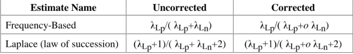
When learning classification trees, differences between rtrainDQG QRUPDOO\UHVXOWLQEiased posterior class-probability estimates at the leaves. To remove this bias, we adjust the probability estimates to take these differences into account. Two simple, common probability estimation

IRUPXODVDUHOLVWHGLQ7DEOH)RUHDFKOHW Lp Ln) represent the number of minority-class

(majority-class) training examples at a leaf L of a decision tree (or, more generally, within any region L). The uncorrected estimates, which are based on the assumption that the training and test sets are drawn from D and approximate , estimate the probability of seeing a minority-class (positive) example in L. The uncorrected frequency-based estimate is straightforward and re-quires no explanation. However, this estimate does not perform well when the sample size,

Lp Ln, is small—and is not even defined when the sample size is 0. For these reasons the

2. For notational convenience we treat L_P and L_N as the union of the sets of instances in the corresponding regions. 3. In situations where it is more costly to misclassify minority-class examples than majority-class examples,

Laplace estimate often is used instead. We consider a version based on the Laplace law of suc-cession (Good, 1965). This probability estimate will always be closer to 0.5 than the frequency-based estimate, but the difference between the two estimates will be negligible for large sample sizes.

Estimate Name Uncorrected Corrected

Frequency-Based _Lp/( _Lp+ _Ln) _Lp _Lp+o _Ln) Laplace (law of succession) Lp+1)/( Lp+ Ln+2) Lp Lp+o Ln+2)

Table 1: Probability Estimates for Observing a Minority-Class Example

The corrected versions of the estimates in Table 1 account for differences between rtrainDQG by factoring in the over-sampling ratio o, which measures the degree to which the minority class is over-sampled in the training set relative to the naturally occurring distribution. The value of o is computed as the ratio of minority-class examples to majority-class examples in the training set divided by the same ratio in the naturally occurring class distribution. If the ratio of minority to majority examples were 1:2 in the training set and 1:6 in the naturally occurring distribution, then o would be 3. A learner can account properly for differences between rtrainDQG E\XVLQJ the corrected estimates to calculate the posterior probabilities at L.

As an example, if the ratio of minority-class examples to majority-class examples in the natu-rally occurring class distribution is 1:5 but the training distribution is modified so that the ratio is 1:1, then o is 1.0/0.2, or 5. For L to be labeled with the minority class the probability must be greater than 0.5, so, using the corrected frequency-EDVHG HVWLPDWH Lp Lp Ln) > 0.5, or, Lp! Ln. Thus, L is labeled with the minority class only if it covers o times as many

minority-class examples as majority-minority-class examples. Note that in calculating o above we use the minority-class ratios and not the fraction of examples belonging to the minority class (if we mistakenly used the latter in the above example, then o would be one-half divided by one-sixth, or 3). Using the class ratios substantially simplifies the formulas and leads to more easily understood estimates. Elkan (2001) provides a more complex, but equivalent, formula that uses fractions instead of ratios. In this discussion we assume that a good approximation of the true base rate is known. In some real-world situations this is not true and different methods are required to compensate for changes to the training set (Provost & Fawcett, 2001; Saerens et al., 2002).

In order to demonstrate the importance of using the corrected estimates, Appendix A presents results comparing decision trees labeled using the uncorrected frequency-based estimate with trees using the corrected frequency-based estimate. This comparison shows that for a particular modification of the class distribution of the training sets (they are modified so that the classes are balanced), using the corrected estimates yields classifiers that substantially outperform classifiers labeled using the uncorrected estimate. In particular, over the twenty-six data sets used in our study, the corrected frequency-based estimate yields a relative reduction in error rate of 10.6%. Furthermore, for only one of the twenty-six data sets does the corrected estimate perform worse. Consequently it is critical to take the differences in the class distributions into account when labeling the leaves. Previous work on modifying the class distribution of the training set (Catlett, 1991; Chan & Stolfo, 1998; Japkowicz, 2002) did not take these differences into account and this undoubtedly affected the results.

4. Experimental Setup

In this section we describe the data sets analyzed in this article, the sampling strategy used to alter the class distribution of the training data, the classifier induction program used, and, finally, the metrics for evaluating the performance of the induced classifiers.

4.1

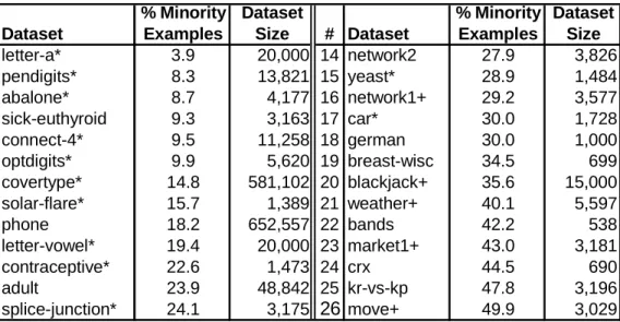
The twenty-six data sets used throughout this article are described in Table 2. This collection includes twenty data sets from the UCI repository (Blake & Merz, 1998), five data sets, identi-fied with a “+”, from previously published work by researchers at AT&T (Cohen & Singer, 1999), and one new data set, the phone data set, generated by the authors. The data sets in Table 2 are listed in order of decreasing class imbalance, a convention used throughout this article.

% Minority Dataset % Minority Dataset

Dataset Examples Size # Dataset Examples Size

letter-a* 3.9 20,000 14 network2 27.9 3,826

pendigits* 8.3 13,821 15 yeast* 28.9 1,484

abalone* 8.7 4,177 16 network1+ 29.2 3,577

sick-euthyroid 9.3 3,163 17 car* 30.0 1,728

connect-4* 9.5 11,258 18 german 30.0 1,000

optdigits* 9.9 5,620 19 breast-wisc 34.5 699

covertype* 14.8 581,102 20 blackjack+ 35.6 15,000

solar-flare* 15.7 1,389 21 weather+ 40.1 5,597

phone 18.2 652,557 22 bands 42.2 538

letter-vowel* 19.4 20,000 23 market1+ 43.0 3,181

contraceptive* 22.6 1,473 24 crx 44.5 690

adult 23.9 48,842 25 kr-vs-kp 47.8 3,196

splice-junction* 24.1 3,175 26 move+ 49.9 3,029

Table 2: Description of Data Sets

In order to simplify the presentation and the analysis of our results, data sets with more than two classes were mapped to two-class problems. This was accomplished by designating one of the original classes, typically the least frequently occurring class, as the minority class and then mapping the remaining classes into the majority class. The data sets that originally contained more than 2 classes are identified with an asterisk (*) in Table 2. The letter-a data set was cre-ated from the letter-recognition data set by assigning the examples labeled with the letter “a” to the minority class; the letter-vowel data set was created by assigning the examples labeled with any vowel to the minority class.

We generated training sets with different class distributions as follows. For each experimen-tal run, first the test set is formed by randomly selecting 25% of the minority-class examples and 25% of the majority-class examples from the original data set, without replacement (the resulting test set therefore conforms to the original class distribution). The remaining data are available for training. To ensure that all experiments for a given data set have the same training-set size— no matter what the class distribution of the training set—the training-set size, S, is made equal to the total number of minority-class examples still available for training (i.e., 75% of the original

number). This makes it possible, without replicating any examples, to generate any class distri-bution for training-set size S. Each training set is then formed by random sampling from the remaining data, without replacement, such that the desired class distribution is achieved. For the experiments described in this article, the class distribution of the training set is varied so that the minority class accounts for between 2% and 95% of the training data.

4.2

The experiments in this article use C4.5, a program for inducing classification trees from labeled examples (Quinlan, 1993). C4.5 uses the uncorrected frequency-based estimate to label the leaves of the decision tree, since it assumes that the training data approximate the true, underly-ing distribution. Given that we modify the class distribution of the trainunderly-ing set, it is essential that we use the corrected estimates to re-label the leaves of the induced tree. The results presented in the body of this article are based on the use of the corrected versions of the frequency-based and Laplace estimates (described in Table 1), using a probability threshold of .5 to label the leaves of the induced decision trees.

C4.5 does not factor in differences between the class distributions of the training and test sets—we adjust for this as a post-processing step. If C4.5’s pruning strategy, which attempts to minimize error rate, were allowed to execute, it would prune based on a false assumption (viz., that the test distribution matches the training distribution). Since this may negatively affect the generated classifier, except where otherwise indicated all results are based on C4.5 without prun-ing. This decision is supported by recent research, which indicates that when target misclassifi-cation costs (or class distributions) are unknown then standard pruning does not improve, and may degrade, generalization performance (Provost & Domingos, 2001; Zadrozny & Elkan, 2001; Bradford et al., 1998; Bauer & Kohavi, 1999). Indeed, Bradford et al. (1998) found that even if the pruning strategy is adapted to take misclassification costs and class distribution into account, this does not generally improve the performance of the classifier. Nonetheless, in order to justify using C4.5 without pruning, we also present the results of C4.5 with pruning when the training set uses the natural distribution. In this situation C4.5’s assumption about rtrainDSSUR[LPDWLQJ is valid and hence its pruning strategy will perform properly. Looking ahead, these results show that C4.5 without pruning indeed performs competitively with C4.5 with pruning.

4.3

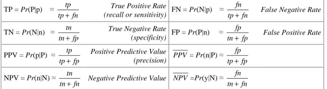
A variety of metrics for assessing classifier performance are based on the terms listed in the con-fusion matrix shown below.

t(x)

Positive Prediction Negative Prediction Actual Positive tp (true positive) fn (false negative) Actual Negative fp (false positive) tn (true negative)

Table 3 summarizes eight such metrics. The metrics described in the first two rows measure the ability of a classifier to classify positive and negative examples correctly, while the metrics described in the last two rows measure the effectiveness of the predictions made by a classifier. For example, the positive predictive value (PPV), or precision, of a classifier measures the frac-tion of positive predicfrac-tions that are correctly classified. The metrics described in the last two

rows of Table 3 are used throughout this article to evaluate how various training-set class distri-butions affect the predictions made by the induced classifiers. Finally, the metrics in the second column of Table 3 are “complements” of the corresponding metrics in the first column, and can alternatively be computed by subtracting the value in the first column from 1. More specifically, proceeding from row 1 through 4, the metrics in column 1 (column 2) represent: 1) the accuracy (error rate) when classifying positive/minority examples, 2) the accuracy (error rate) when classi-fying negative/minority examples, 3) the accuracy (error rate) of the positive/minority predic-tions, and 4) the accuracy (error rate) of the negative/majority predictions.

TP = Pr(P|p) § fn tp

tp

+

True Positive Rate

(recall or sensitivity) FN = Pr(N|p) § tp fn fn

+ False Negative Rate

TN = Pr(N|n) § fp tn

tn

+

True Negative Rate

(specificity) FP = Pr(P|n) § tn fp fp

+ False Positive Rate

PPV = Pr(p|P) § fp tp

tp

+

Positive Predictive Value

(precision) PPV= Pr(n|P) § _{tp fp} fp

+

NPV = Pr(n|N) § fn tn

tn

+ Negative Predictive Value NPV =Pr(y|N) § tn fn fn

+

Table 3: Classifier Performance Metrics

We use two performance measures to gauge the overall performance of a classifier: classifica-tion accuracy and the area under the ROC curve (Bradley, 1997). Classificaclassifica-tion accuracy is (tp+

fp)/(tp+fp+tn+fn). This formula, which represents the fraction of examples that are correctly FODVVLILHGLVDQHVWLPDWHRIWKHH[SHFWHGDFFXUDF\ t, defined earlier in equation 1. Throughout this article we specify classification accuracy in terms of error rate, which is 1–accuracy.

We consider classification accuracy in part because it is the most common evaluation metric in machine-learning research. However, using accuracy as a performance measure assumes that the target (marginal) class distribution is known and unchanging and, more importantly, that the error costs—the costs of a false positive and false negative—are equal. These assumptions are unrealistic in many domains (Provost et al., 1998). Furthermore, highly unbalanced data sets typically have highly non-uniform error costs that favor the minority class, which, as in the case of medical diagnosis and fraud detection, is the class of primary interest. The use of accuracy in these cases is particularly suspect since, as we discuss in Section 5.2, it is heavily biased to favor the majority class and therefore will sometimes generate classifiers that never predict the minor-ity class. In such cases, Receiver Operating Characteristic (ROC) analysis is more appropriate (Swets et al., 2000; Bradley, 1997; Provost & Fawcett, 2001). When producing the ROC curves we use the Laplace estimate to estimate the probabilities at the leaves, since it has been shown to yield consistent improvements (Provost & Domingos, 2001). To assess the overall quality of a classifier we measure the fraction of the total area that falls under the ROC curve (AUC), which is equivalent to several other statistical measures for evaluating classification and ranking models (Hand, 1997). Larger AUC values indicate generally better classifier performance and, in par-ticular, indicate a better ability to rank cases by likelihood of class membership.

5. Learning from Unbalanced Data Sets

We now analyze the classifiers induced from the twenty-six naturally unbalanced data sets de-scribed in Table 2, focusing on the differences in performance for the minority and majority classes. We do not alter the class distribution of the training data in this section, so the classifi-ers need not be adjusted using the method described in Section 3. However, so that these ex-periments are consistent with those in Section 6 that use the natural distribution, the size of the training set is reduced, as described in Section 4.1.

Before addressing these differences, it is important to discuss an issue that may lead to confu-sion if left untreated. Practitioners have noted that learning performance often is unsatisfactory when learning from data sets where the minority class is substantially underrepresented. In par-ticular, they observe that there is a large error rate for the minority class. As should be clear from Table 3 and the associated discussion, there are two different notions of “error rate for the minority class”: the minority-class predictions could have a high error rate (largePPV ) or the minority-class test examples could have a high error rate (large FN). When practitioners observe that the error rate is unsatisfactory for the minority class, they are usually referring to the fact that the minority-class examples have a high error rate (large FN). The analysis in this section will show that the error rate associated with the minority-class predictions (PPV ) and the minor-ity-classtestexamples(FN)botharemuch larger than their majority-classcounterparts (NPVand

FP, respectively). We discuss several explanations for these observed differences.

5.1

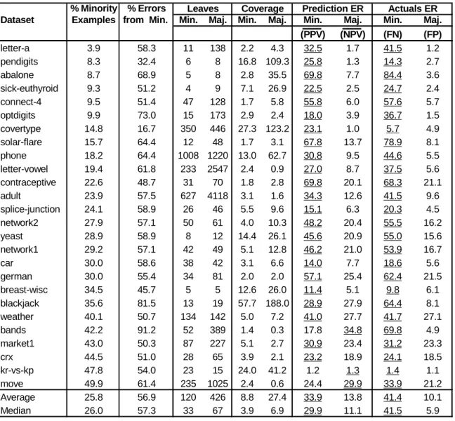
The performances of the classifiers induced from the twenty-six unbalanced data sets are de-scribed in Table 4. This table warrants some explanation. The first column specifies the data set name while the second column, which for convenience has been copied from Table 2, specifies the percentage of minority-class examples in the natural class distribution. The third column specifies the percentage of the total test errors that can be attributed to the test examples that belong to the minority class. By comparing the values in columns two and three we see that in all cases a disproportionately large percentage of the errors come from the minority-class exam-ples. For instance, minority-class examples make up only 3.9% of the letter-a data set but con-tribute 58.3% of the errors. Furthermore, for 22 of 26 data sets a majority of the errors can be attributed to minority-class examples.

The fourth column specifies the number of leaves labeled with the minority and majority classes and shows that in all but two cases there are fewer leaves labeled with the minority class than with the majority class. The fifth column, “Coverage,” specifies the average number of training examples that eachminority-labeled or majority-labeled leafclassifies (“covers”). These results indicate that the leaveslabeled with the minority class are formed from far fewer training examples than those labeled with the majority class.

The “Prediction ER” column specifies the error rates associated with the minority-class and majority-class predictions, based on the performance of these predictions at classifying the test examples. The “Actuals ER” column specifies the classification error rates for the minority and majority class examples, again based on the test set. These last two columns are also labeled using the terms defined in Section 2 (PPV,NPV, FN, and FP). As an example, these columns show that for the letter-a data set the minority-labeled predictions have an error rate of 32.5% while the majority-labeled predictions have an error rate of only 1.7%, and that the minority-class test examples have a minority-classification error rate of 41.5% while the majority-minority-class test

exam-ples have an error rate of only 1.2%. In each of the last two columns we underline the higher error rate.

% Minority % Errors

Dataset Examples from Min. Min. Maj. Min. Maj. Min. Maj. Min. Maj. (PPV) (NPV) (FN) (FP)

letter-a 3.9 58.3 11 138 2.2 4.3 32.5 1.7 41.5 1.2

pendigits 8.3 32.4 6 8 16.8 109.3 25.8 1.3 14.3 2.7

abalone 8.7 68.9 5 8 2.8 35.5 69.8 7.7 84.4 3.6

sick-euthyroid 9.3 51.2 4 9 7.1 26.9 22.5 2.5 24.7 2.4

connect-4 9.5 51.4 47 128 1.7 5.8 55.8 6.0 57.6 5.7

optdigits 9.9 73.0 15 173 2.9 2.4 18.0 3.9 36.7 1.5

covertype 14.8 16.7 350 446 27.3 123.2 23.1 1.0 5.7 4.9

solar-flare 15.7 64.4 12 48 1.7 3.1 67.8 13.7 78.9 8.1

phone 18.2 64.4 1008 1220 13.0 62.7 30.8 9.5 44.6 5.5

letter-vowel 19.4 61.8 233 2547 2.4 0.9 27.0 8.7 37.5 5.6

contraceptive 22.6 48.7 31 70 1.8 2.8 69.8 20.1 68.3 21.1

adult 23.9 57.5 627 4118 3.1 1.6 34.3 12.6 41.5 9.6

splice-junction 24.1 58.9 26 46 5.5 9.6 15.1 6.3 20.3 4.5

network2 27.9 57.1 50 61 4.0 10.3 48.2 20.4 55.5 16.2

yeast 28.9 58.9 8 12 14.4 26.1 45.6 20.9 55.0 15.6

network1 29.2 57.1 42 49 5.1 12.8 46.2 21.0 53.9 16.7

car 30.0 58.6 38 42 3.1 6.6 14.0 7.7 18.6 5.6

german 30.0 55.4 34 81 2.0 2.0 57.1 25.4 62.4 21.5

breast-wisc 34.5 45.7 5 5 12.6 26.0 11.4 5.1 9.8 6.1

blackjack 35.6 81.5 13 19 57.7 188.0 28.9 27.9 64.4 8.1

weather 40.1 50.7 134 142 5.0 7.2 41.0 27.7 41.7 27.1

bands 42.2 91.2 52 389 1.4 0.3 17.8 34.8 69.8 4.9

market1 43.0 50.3 87 227 5.1 2.7 30.9 23.4 31.2 23.3

crx 44.5 51.0 28 65 3.9 2.1 23.2 18.9 24.1 18.5

kr-vs-kp 47.8 54.0 23 15 24.0 41.2 1.2 1.3 1.4 1.1

move 49.9 61.4 235 1025 2.4 0.6 24.4 29.9 33.9 21.2

Average 25.8 56.9 120 426 8.8 27.4 33.9 13.8 41.4 10.1

Median 26.0 57.3 33 67 3.9 6.9 29.9 11.1 41.5 5.9

Leaves Coverage Prediction ER Actuals ER

Table 4: Behavior of Classifiers Induced from Unbalanced Data Sets

The results in Table 4 clearly demonstrate that the minority-class predictions perform much worse than the majority-class predictions and that the minority-class examples are misclassified much more frequently than majority-class examples. Over the twenty-six data sets, the minority predictions have an average error rate (PPV) of 33.9% while the majority-class predictions have an average error rate (NPV) of only 13.8%. Furthermore, for only three of the twenty-six data sets do the majority-class predictions have a higher error rate—and for these three data sets the class distributions are only slightly unbalanced. Table 4 also shows us that the average error rate for the minority-class test examples (FN) is 41.4% whereas for the majority-class test examples the error rate (FP) is only 10.1%. In every one of the twenty-six cases the minority-class test examples have a higher error rate than the majority-class test examples.

5.2

Why do the minority-class predictions have a higher error rate (PPV)than the majority-class predictions (NPV)? There are at least two reasons. First, consider a classifier trandom where the partitions L are chosen randomly and the assignment of each L ∈L to LP and LN is also made randomly (recall that LP and LN represent the regions labeled with the positive and negative classes). For a two-class learning problem WKHH[SHFWHGRYHUDOODFFXUDF\ t, of this randomly generated and labeled classifier must be 0.5. However, the expected accuracy of the regions in the positive partiWLRQ L_PZLOOEH ZKLOHWKHH[SHFWHGDFFXUDF\RIWKHUHJLRQVLQWKHQHJDWLYH

partition, _LN, will be 1 – )RUDKLJKO\XQEDODQFHGFODVVGLVWULEXWLRQZKHUH _LP=.01

DQG L_N = .99. Thus, in such a scenario the negative/majority predictions will be much more

“accurate.” While this “test distribution effect” will be small for a well-learned concept with a low Bayes error rate (and non-existent for a perfectly learned concept with a Bayes error rate of 0), many learning problems are quite hard and have high Bayes error rates.4

The results in Table 4 suggest a second explanation for why the minority-class predictions are so error prone. According to the coverage results, minority-labeled predictions tend to be formed from fewer training examples than majority-labeled predictions. Small disjuncts, which are the components of disjunctive concepts (i.e., classification rules, decision-tree leaves, etc.) that cover few training examples, have been shown to have a much higher error rate than large disjuncts (Holte, et al., 1989; Weiss & Hirsh, 2000). Consequently, the rules/leaves labeled with the mi-nority class have a higher error rate partly because they suffer more from this “problem of small disjuncts.”

Next, why are minority-class examples classified incorrectly much more often than majority-class examples (FN > FP)—a phenomenon that has also been observed by others (Japkowicz & Stephen, 2002)? Consider the estimated accuracy, a_t, of a classifier t, where the test set is drawn from the true, underlying distribution D:

a_t = TP • rtest + TN • (1 – rtest) [2] Since the positive class corresponds to the minority class, rtest < .5, and for highly unbalanced data sets r_test << .5. Therefore, false-positive errors are more damaging to classification accuracy than false negative errors are. A classifier that is induced using an induction algorithm geared toward maximizing accuracy therefore should “prefer” false-negative errors over false-positive errors. This will cause negative/majority examples to be predicted more often and hence will lead to a higher error rate for minority-class examples. One straightforward example of how learning algorithms exhibit this behavior is provided by the common-sense rule: if there is no evidence favoring one classification over another, then predict the majority class. More gener-ally, induction algorithms that maximize accuracy should be biased to perform better at classify-ing majority-class examples than minority-class examples, since the former component is weighted more heavily when calculating accuracy. This also explains why, when learning from data sets with a high degree of class imbalance, classifiers rarely predict the minority class.

A second reason why minority-class examples are misclassified more often than majority-class examples is that fewer minority-majority-class examples are likely to be sampled from the

4. The (optimal) Bayes error rate, using the terminology from Section 2, occurs when t(.)=c(.). Because c(.) may be probabilistic (e.g., when noise is present), the Bayes error rate for a well-learned concept may not always be low. The test distribution effect will be small when the concept is well learned and the Bayes error rate is low.

tion D. Therefore, the training data are less likely to include (enough) instances of all of the minority-class subconcepts in the concept space, and the learner may not have the opportunity to represent all truly positive regions in LP. Because of this, some minority-class test examples will be mistakenly classified as belonging to the majority class.

Finally, it is worth noting that PPV> NPV does not imply that FN > FP. That is, having more error-prone minority predictions does not imply that the minority-class examples will be misclassified more often than majority-class examples. Indeed, a higher error rate for minority predictions means more majority-class test examples will be misclassified. The reason we gen-erally observe a lower error rate for the majority-class test examples (FN > FP) is because the majority class is predicted far more often than the minority class.

6. The Effect of Training-Set Class Distribution on Classifier Performance

We now turn to the central questions of our study: how do different training-set class distribu-tions affect the performance of the induced classifiers and which class distribudistribu-tions lead to the best classifiers? We begin by describing the methodology for determining which class distribu-tion performs best. Then, in the next two secdistribu-tions, we evaluate and analyze classifier perform-ance for the twenty-six data sets using a variety of class distributions. We use error rate as the performance metric in Section 6.2 and AUC as the performance metric in Section 6.3.

6.1

In order to evaluate the effect of class distribution on classifier performance, we vary the train-ing-set class distributions for the twenty-six data sets using the methodology described in Section 4.1. We evaluate the following twelve class distributions (expressed as the percentage of minor-ity-class examples): 2%, 5%, 10%, 20%, 30%, 40%, 50%, 60%, 70%, 80%, 90%, and 95%. For each data set we also evaluate the performance using the naturally occurring class distribution.

Before we try to determine the “best” class distribution for a training set, there are several is-sues that must be addressed. First, because we do not evaluate every possible class distribution, we can only determine the best distribution among the 13 evaluated distributions. Beyond this concern, however, is the issue of statistical significance and, because we generate classifiers for 13 training distributions, the issue of multiple comparisons (Jensen & Cohen, 2000). Because of these issues we cannot always conclude that the distribution that yields the best performing clas-sifiers is truly the best one for training.

We take several steps to address the issues of statistical significance and multiple compari-sons. To enhance our ability to identify true differences in classifier performance with respect to changes in class distribution, all results presented in this section are based on 30 runs, rather than the 10 runs employed in Section 5. Also, rather than trying to determine the best class distribu-tion, we adopt a more conservative approach, and instead identify an “optimal range” of class distributions—a range in which we are confident the best distribution lies. To identify the opti-mal range of class distributions, we begin by identifying, for each data set, the class distribution that yields the classifiers that perform best over the 30 runs. We then perform t-tests to compare the performance of these 30 classifiers with the 30 classifiers generated using each of the other twelve class distributions (i.e., 12 t-tests each with n=30 data points). If a t-test yields a probabil-ity ≤ .10 then we conclude that the “best” distribution is different from the “other” distribution (i.e., we are at least 90% confident of this); otherwise we cannot conclude that the class distribu-tions truly perform differently and therefore “group” the distribudistribu-tions together. These grouped

distributions collectively form the “optimal range” of class distributions. As Tables 5 and 6 will show, in 50 of 52 cases the optimal ranges are contiguous, assuaging concerns that our conclu-sions are due to problems of multiple comparisons.

6.2

Table 5 displays the error rates of the classifiers induced for each of the twenty-six data sets. The first column in Table 5 specifies the name of the data set and the next two columns specify the error rates that result from using the natural distribution, with and then without pruning. The next 12 columns present the error rate values for the 12 fixed class distributions (without prun-ing). For each data set, the “best” distribution (i.e., the one with the lowest error rate) is high-lighted by underlining it and displaying it in boldface. The relative position of the natural distribution within the range of evaluated class distributions is denoted by the use of a vertical bar between columns. For example, for the letter-a data set the vertical bar indicates that the natural distribution falls between the 2% and 5% distributions (from Table 2 we see it is 3.9%).

Dataset

Nat-Prune Nat 2 5 10 20 30 40 50 60 70 80 90 95 best vs. nat best vs. bal

letter-a 2.80 x 2.78 2.86 2.75 2.59 3.03 3.79 4.53 5.38 6.48 8.51 12.37 18.10 26.14 6.8 51.9

pendigits 3.65 + 3.74 5.77 3.95 3.63 3.45 3.70 3.64 4.02 4.48 4.98 5.73 8.83 13.36 7.8 14.2

abalone 10.68 x 10.46 9.04 9.61 10.64 13.19 15.33 20.76 22.97 24.09 26.44 27.70 27.73 33.91 13.6 60.6

sick-euthyroid 4.46 x 4.10 5.78 4.82 4.69 4.25 5.79 6.54 6.85 9.73 12.89 17.28 28.84 40.34 0.0 40.1

connect-4 10.68 x 10.56 7.65 8.66 10.80 15.09 19.31 23.18 27.57 33.09 39.45 47.24 59.73 72.08 27.6 72.3

optdigits 4.94 x 4.68 8.91 7.01 4.05 3.05 2.83 2.79 3.41 3.87 5.15 5.75 9.72 12.87 40.4 18.2

covertype 5.12 x 5.03 5.54 5.04 5.00 5.26 5.64 5.95 6.46 7.23 8.50 10.18 13.03 16.27 0.6 22.6

solar-flare 19.16 + 19.98 16.54 17.52 18.96 21.45 23.03 25.49 29.12 30.73 33.74 38.31 44.72 52.22 17.2 43.2

phone 12.63 x 12.62 13.45 12.87 12.32 12.68 13.25 13.94 14.81 15.97 17.32 18.73 20.24 21.07 2.4 16.8

letter-vowel 11.76 x 11.63 15.87 14.24 12.53 11.67 12.00 12.69 14.16 16.00 18.68 23.47 32.20 41.81 0.0 17.9

contraceptive 31.71 x 30.47 24.09 24.57 25.94 30.03 32.43 35.45 39.65 43.20 47.57 54.44 62.31 67.07 20.9 39.2

adult 17.42 x 17.25 18.47 17.26 16.85 17.09 17.78 18.85 20.05 21.79 24.08 27.11 33.00 39.75 2.3 16.0

splice-junction 8.30 + 8.37 20.00 13.95 10.72 8.68 8.50 8.15 8.74 9.86 9.85 12.08 16.25 21.18 2.6 6.8 network2 27.13 x 26.67 27.37 25.91 25.71 25.66 26.94 28.65 29.96 32.27 34.25 37.73 40.76 37.72 3.8 14.4

yeast 26.98 x 26.59 29.08 28.61 27.51 26.35 26.93 27.10 28.80 29.82 30.91 35.42 35.79 36.33 0.9 8.5

network1 27.57 + 27.59 27.90 27.43 26.78 26.58 27.45 28.61 30.99 32.65 34.26 37.30 39.39 41.09 3.7 14.2

car 9.51 x 8.85 23.22 18.58 14.90 10.94 8.63 8.31 7.92 7.35 7.79 8.78 10.18 12.86 16.9 7.2 german 33.76 x 33.41 30.17 30.39 31.01 32.59 33.08 34.15 37.09 40.55 44.04 48.36 55.07 60.99 9.7 18.7

breast-wisc 7.41 x 6.82 20.65 14.04 11.00 8.12 7.49 6.82 6.74 7.30 6.94 7.53 10.02 10.56 1.2 0.0 blackjack 28.14 + 28.40 30.74 30.66 29.81 28.67 28.56 28.45 28.71 28.91 29.78 31.02 32.67 33.87 0.0 1.1 weather 33.68 + 33.69 38.41 36.89 35.25 33.68 33.11 33.43 34.61 36.69 38.36 41.68 47.23 51.69 1.7 4.3

bands 32.26 + 32.53 38.72 35.87 35.71 34.76 33.33 32.16 32.68 33.91 34.64 39.88 40.98 40.80 1.1 1.6 market1 26.71 x 26.16 34.26 32.50 29.54 26.95 26.13 26.05 25.77 26.86 29.53 31.69 36.72 39.90 1.5 0.0 crx 20.99 x 20.39 35.99 30.86 27.68 23.61 20.84 20.82 21.48 21.64 22.20 23.98 28.09 32.85 0.0 5.1

kr-vs-kp 1.25 + 1.39 12.18 6.50 3.20 2.33 1.73 1.16 1.22 1.34 1.53 2.55 3.66 6.04 16.5 4.9 move 27.54 + 28.57 46.13 42.10 38.34 33.48 30.80 28.36 28.24 29.33 30.21 31.80 36.08 40.95 1.2 0.0

Error Rate when using Specified Training Distribution (training distribution expressed as % minority)

Relative % Improvement

The error rate values that are not significantly different, statistically, from the lowest error rate (i.e., the comparison yields a t-test value > .10) are shaded. Thus, for the letter-a data set, the optimum range includes those class distributions that include between 2% and 10% minority-class examples—which includes the natural distribution. The last two columns in Table 5 show the relative improvement in error rate achieved by using the best distribution instead of the natu-ral and balanced distributions. When this improvement is statistically significant (i.e., is associ-ated with a t-test value ≤ .10) then the value is displayed in bold.

The results in Table 5 show that for 9 of the 26 data sets we are confident that the natural dis-tribution is not within the optimal range. For most of these 9 data sets, using the best disdis-tribution rather than the natural distribution yields a remarkably large relative reduction in error rate. We feel that this is sufficient evidence to conclude that for accuracy, when the training-set size must be limited, it is not appropriate simply to assume that the natural distribution should be used. Inspection of the error-rateresultsin Table 5 also showsthatthebestdistributiondoesnot differ from the natural distribution in any consistent manner—sometimes it includes more minority-class examples (e.g., optdigits, car) and sometimes fewer (e.g., connect-4, solar-flare). However, it is clear that for data sets with a substantial amount of class imbalance (the ones in the top half of the table), a balanced class distribution also is not the best class distribution for training, to minimize undifferentiated error rate. More specifically, none of the top-12 most skewed data sets have the balanced class distribution within their respective optimal ranges, and for these data sets the relative improvements over the balanced distributions are striking.

Let us now consider the error-rate values for the remaining 17 data sets for which the t-test re-sults do not permit us to conclude that the best observed distribution truly outperforms the natu-ral distribution. In these cases we see that the error rate values for the 12 training-set class distributions usually form a unimodal, or nearly unimodal, distribution. This is the distribution one would expect if the accuracy of a classifier progressively degrades the further it deviates from the best distribution. This suggests that “adjacent” class distributions may indeed produce classifiers that perform differently, but that our statistical testing is not sufficiently sensitive to identify these differences. Based on this, we suspect that many of the observed improvements shown in the last column of Table 5 that are not deemed to be significant statistically are none-theless meaningful.

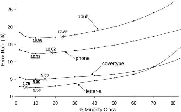
Figure 1 shows the behavior of the learned classifiers for the adult, phone, covertype, and let-ter-a data sets in a graphical form. In this figure the natural distribution is denoted by the “X” tick mark and the associated error rate is noted above the marker. The error rate for the best distribution is underlined and displayed below the corresponding data point (for these four data sets the best distribution happens to include 10% minority-class examples). Two of the curves are associated with data sets (adult, phone) for which we are >90% confident that the best distri-bution performs better than the natural distridistri-bution, while for the other two curves (covertype, letter-a) we are not. Note that all four curves are perfectly unimodal. It is also clear that near the distribution that minimizes error rate, changes to the class distribution yield only modest changes in the error rate—far more dramatic changes occur elsewhere. This is also evident for most data sets in Table 5. This is a convenient property given the common goal of minimizing error rate. This property would be far less evident if the correction described in Section 3 were not per-formed, since then classifiers induced from class distributions deviating from the naturally occur-ring distribution would be improperly biased.

2.75 2.59

17.25 16.85

12.32 12.62

5.00 5.03

0 5 10 15 20 25

0 10 20 30 40 50 60 70 80

% Minority Class

Error Rate (%)

letter-a adult

phone

covertype

Figure 1: Effect of Class Distribution on Error Rate for Select Data Sets

Finally, to assess whether pruning would have improved performance, consider the second column in Table 5, which displays the error rates that result from using C4.5 with pruning on the natural distribution (recall from Section 4.2 that this is the only case when C4.5’s pruning strat-egy will give unbiased results). A “+”/“x” in the second column indicates that C4.5 with pruning outperforms/underperforms C4.5 without pruning, when learning from the natural distribution. Note that C4.5 with pruning underperforms C4.5 without pruning for 17 of the 26 data sets, which leads us to conclude that C4.5 without pruning is a reasonable learner. Furthermore, in no case does C4.5 with pruning generate a classifier within the optimal range when C4.5 without pruning does not also generate a classifier within this range.

6.3

The performance of the induced classifiers, using AUC as the performance measure, is displayed in Table 6. When viewing these results, recall that for AUC larger values indicate improved performance. The relative improvement in classifier performance is again specified in the last two columns, but now the relative improvement in performance is calculated in terms of the area above the ROC curve (i.e., 1 – AUC). We use the area above the ROC curve because it better reflects the relative improvement—just as in Table 5 relative improvement is specified in terms of the change in error rate instead of the change in accuracy. As before, the relative improve-ments are shown in bold only if we are more than 90% confident that they reflect a true im-provement in performance (i.e., t-test value ”

In general, the optimum ranges appear to be centered near, but slightly to the right, of the bal-anced class distribution. For 12 of the 26 data sets the optimum range does not include the natu-ral distribution (i.e., the third column is not shaded). Note that for these data sets, with the exception of the solar-flare data set, the class distributions within the optimal range contain more minority-class examples than the natural class distribution. Based on these results we conclude even more strongly for AUC (i.e., for cost-sensitive classification and for ranking) than for

accu-racy that it is not appropriate simply to choose the natural class distribution for training. Table 6 also shows that, unlike for accuracy, a balanced class distribution generally performs very well, although it does not always perform optimally. In particular, we see that for 19 of the 26 data sets the balanced distribution is within the optimal range. This result is not too surprising since AUC, unlike error rate, is unaffected by the class distribution of the test set, and effectively fac-tors in classifier performance over all class distributions.

Dataset

Nat-prune Nat 2 5 10 20 30 40 50 60 70 80 90 95 best vs. nat best vs. bal

letter-a .500 x .772 .711 .799 .865 .891 .911 .938 .937 .944 .951 .954 .952 .940 79.8 27.0 pendigits .962 x .967 .892 .958 .971 .976 .978 .979 .979 .978 .977 .976 .966 .957 36.4 0.0 abalone .590 x .711 .572 .667 .710 .751 .771 .775 .776 .778 .768 .733 .694 .687 25.8 0.9 sick-euthyroid .937 x .940 .892 .908 .933 .943 .944 .949 .952 .951 .955 .945 .942 .921 25.0 6.3 connect-4 .658 x .731 .664 .702 .724 .759 .763 .777 .783 .793 .793 .789 .772 .730 23.1 4.6 optdigits .659 x .803 .599 .653 .833 .900 .924 .943 .948 .959 .967 .965 .970 .965 84.8 42.3 covertype .982 x .984 .970 .980 .984 .984 .983 .982 .980 .978 .976 .973 .968 .960 0.0 20.0 solar-flare .515 x .627 .614 .611 .646 .627 .635 .636 .632 .650 .662 .652 .653 .623 9.4 8.2 phone .850 x .851 .843 .850 .852 .851 .850 .850 .849 .848 .848 .850 .853 .850 1.3 2.6 letter-vowel .806 + .793 .635 .673 .744 .799 .819 .842 .849 .861 .868 .868 .858 .833 36.2 12.6 contraceptive .539 x .611 .567 .613 .617 .616 .622 .640 .635 .635 .640 .641 .627 .613 7.7 1.6 adult .853 + .839 .816 .821 .829 .836 .842 .846 .851 .854 .858 .861 .861 .855 13.7 6.7 splice-junction .932 + .905 .814 .820 .852 .908 .915 .925 .936 .938 .944 .950 .944 .944 47.4 21.9 network2 .712 + .708 .634 .696 .703 .708 .705 .704 .705 .702 .706 .710 .719 .683 3.8 4.7 yeast .702 x .705 .547 .588 .650 .696 .727 .714 .720 .723 .715 .699 .659 .621 10.9 2.5 network1 .707 + .705 .626 .676 .697 .709 .709 .706 .702 .704 .708 .713 .709 .696 2.7 3.7 car .931 + .879 .754 .757 .787 .851 .884 .892 .916 .932 .931 .936 .930 .915 47.1 23.8 german .660 + .646 .573 .600 .632 .615 .635 .654 .645 .640 .650 .645 .643 .613 2.3 2.5 breast-wisc .951 x .958 .876 .916 .940 .958 .963 .968 .966 .963 .963 .964 .949 .948 23.8 5.9 blackjack .682 x .700 .593 .596 .628 .678 .688 .712 .713 .715 .700 .678 .604 .558 5.0 0.7 weather .748 + .736 .694 .715 .728 .737 .738 .740 .736 .730 .736 .722 .718 .702 1.5 1.5 bands .604 x .623 .522 .559 .564 .575 .599 .620 .618 .604 .601 .530 .526 .536 0.0 1.3 market1 .815 + .811 .724 .767 .785 .801 .810 .808 .816 .817 .812 .805 .795 .781 3.2 0.5 crx .889 + .852 .804 .799 .805 .817 .834 .843 .853 .845 .857 .848 .853 .866 9.5 8.8 kr-vs-kp .996 x .997 .937 .970 .991 .994 .997 .998 .998 .998 .997 .994 .988 .982 33.3 0.0 move .762 + .734 .574 .606 .632 .671 .698 .726 .735 .738 .742 .736 .711 .672 3.0 2.6

(training distribution expressed as % minority)

AUC when using Specified Training Distribution Relative %

Improv. (1-AUC)

Table 6: Effect of Training Set Class Distribution on AUC

If we look at the results with pruning, we see that for 15 of the 26 data sets C4.5 with pruning underperforms C4.5 without pruning. Thus, with respect to AUC, C4.5 without pruning is a reasonable learner. However, note that for the car data set the natural distribution with pruning falls into the optimum range, whereas without pruning it does not.

Figure 2 shows how class distribution affects AUC for the adult, covertype, and letter-a data sets (the phone data set is not displayed as it was in Figure 1 because it would obscure the adult data set). Again, the natural distribution is denoted by the “X” tick mark. The AUC for the best distribution is underlined and displayed below the corresponding data point. In this case we also see that near the optimal class distribution the AUC curves tend to be flatter, and hence less sen-sitive to changes in class distribution.

.772

.954

.839 _{.861 .861}

.984 .984 .984

0.7 0.8 0.9 1.0

0 10 20 30 40 50 60 70 80 90

% Minority Class

AUC

letter-a

adult

covertype

Figure 2: Effect of Class Distribution on AUC for Select Data Sets

Figure 3 shows several ROC curves associated with the letter-vowel data set. These curves each were generated from a single run of C4.5 (which is why the AUC values do not exactly match the values in Table 6). In ROC space, the point (0,0) corresponds to the strategy of never making a positive/minority prediction and the point (1,1) to always predicting the positive/minority class. Points to the “northwest” indicate improved performance.

0.0 0.2 0.4 0.6 0.8 1.0

0.0 0.2 0.4 0.6 0.8 1.0

False Positive Rate

T

ru

e

Po

sitive

Ra

te

2% Minority

19% Minority (Natural) 50% Minority

90% Minority

% Minority AUC 2% .599 19% .795 50% .862 90% .855

Observe that different training distributions perform better in different areas of ROC space. Specifically note that the classifier trained with 90% minority-class examples performs substan-tially better than the classifier trained with the natural distribution for high true-positive rates and that the classifier training with 2% minority-class examples performs fairly well for low true-positive rates. Why? With only a small sample of minority-class examples (2%) a classifier can identify only a few minority-labeled “rules” with high confidence. However, with a much larger sample of minority-class examples (90%) it can identify many more such minority-labeled rules. However, for this data set a balanced distribution has the largest AUC and performs best overall. Note that the curve generated using the balanced class distribution almost always outperforms the curve associated with the natural distribution (for low false-positive rates the natural distribu-tion performs slightly better).

7. Forming a Good Class Distribution with Sensitivity to Procurement Costs

The results from the previous section demonstrate that some marginal class distributions yield classifiers that perform substantially better than the classifiers produced by other training distri-butions. Unfortunately, in order to determine the best class distribution for training, forming all thirteen training sets of size n, each with a different class distribution, requires nearly 2n exam-ples. When it is costly to obtain training examples in a form suitable for learning, then this ap-proach is self-defeating. Ideally, given a budget that allows for n training examples, one would select a total of n training examples all of which would be used in the final training set—and the associated class distribution would yield classifiers that perform better than those generated from any other class distribution (given n training examples). In this section we describe and evaluate a heuristic, budget-sensitive, progressive sampling algorithm that approximates this ideal.

In order to evaluate this progressive sampling algorithm, it is necessary to measure how class distribution affects classifier performance for a variety of different training-set sizes. These measurements are summarized in Section 7.1 (the detailed results are included in Appendix B). The algorithm for selecting training data is then described in Section 7.2 and its performance evaluated in Section 7.3, using the measurements included in Appendix B.

7.1 The Effect of Class Distribution and Training-Set Size on Classifier Performance

Experiments were run to establish the relationship between class distribution, training-set size and classifier performance. In order to ensure that the training sets contain a sufficient number of training examples to provide meaningful results when the training-set size is dramatically re-duced, only the data sets that yield relatively large training sets are used (this is determined based on the size of the data set and the fraction of minority-class examples in the data set). Based on this criterion, the following seven data sets were selected for analysis: phone, adult, covertype, blackjack, kr-vs-kp, letter-a, and weather. The detailed results associated with these experiments are contained in Appendix B.

The results for one of these data sets, the adult data set, are shown graphically in Figure 4 and Figure 5, which show classifier performance using error rate and AUC, respectively. Each of the nine performance curves in these figures is associated with a specific training-set size, which contains between 1/128 and all of the training data available for learning (using the methodology described in Section 4.1). Because the performance curves always improve with increasing data-set size, only the curves corresponding to the smallest and largest training-data-set sizes are explicitly labeled.

15 20 25 30 35

0 10 20 30 40 50 60 70 80

% Minority Examples in Training Set

Error Rate

1/128 1/64 1/32 1/16 1/8 1/4 1/2 3/4 1

1/128

1 (all available training data) Natural

Figure 4: Effect of Class Distribution and Training-set Size on Error Rate (Adult Data Set)

0.5 0.6 0.7 0.8 0.9

0 10 20 30 40 50 60 70 80 90 100

% Minority Class Examples in Training Set

AU

C

Natural 1 (all available training data)

1/128

Figure 4 and Figure 5 show several important things. First, while a change in training-set size shifts the performance curves, the relative rank of each point on each performance curve remains roughly the same. Thus, while the class distribution that yields the best performance occasion-ally varies with training-set size, these variations are relatively rare and when they occur, they are small. For example, Figure 5 (and the supporting details in Appendix B) indicates that for the adult data set, the class distribution that yields the best AUC typically contains 80% minority-class examples, although there is occasionally a small deviation (with 1/8 the training data 70% minority-class examples does best). This gives support to the notion that there may be a “best” marginal class distribution for a learning task and suggests that a progressive sampling algorithm may be useful in locating the class distribution that yields the best, or nearly best, classifier per-formance.

The results also indicate that, for any fixed class distribution, increasing the size of the train-ing set always leads to improved classifier performance. Also note that the performance curves tend to “flatten out” as the size of the data set grows, indicating that the choice of class distribu-tion may become less important as the training-set size grows. Nonetheless, even when all of the available training data are used, the choice of class distribution does make a difference. This is significant because if a plateau had been reached (i.e., learning had stopped), then it would be possible to reduce the size of the training set without degrading classifier performance. In that case it would not be necessary to select the class distribution of the training data carefully.

The results in Figure 4 and Figure 5 also show that by carefully selecting the class distribu-tion, one can sometimes achieve improved performance while using fewer training examples. To see this, consider the dashed horizontal line in Figure 4, which intersects the curve associated with ¾ of the training data at its lowest error rate, when the class distribution includes 10% mi-nority-class examples. When this horizontal line is below the curve associated with all available training data, then the training set with ¾ of the data outperforms the full training set. In this case we see that ¾ of the training data with a 10% class distribution outperforms the natural class distribution using all of the available training data. The two horizontal lines in Figure 5 highlight just some of the cases where one can achieve improved AUC using fewer training data (because larger AUC values indicate improved performance, compare the horizontal lines with the curves that lie above them). For example, Figure 5 shows that the training set with a class distribution that contains 80% minority-class examples and 1/128th of the total training data outperforms a training set with twice the training data when its class distribution contains less than or equal to 40% minority-class examples (and outperforms a training set with four times the data if its class distribution contains less than or equal to 10% minority-class examples). The results in Appen-dix B show that all of the trends noted for the adult data set hold for the other data sets and that one can often achieve improved performance using less training data.

7.2 A Budget-Sensitive Progressive sampling Algorithm for Selecting Training Data

As discussed above, the size of the training set sometimes must be limited due to costs associated with procuring usable training examples. For simplicity, assume that there is a budget n, which permits one to procure exactly n training examples. Further assume that the number of training examples that potentially can be procured is sufficiently large so that a training set of size n can be formed with any desired marginal class distribution. We would like a sampling strategy that selects x minority-class examples and y majority-class examples, where x + y = n, such that the

resulting class distribution yields the best possible classification performance for a training set of size n.

The sampling strategy relies on several assumptions. First, we assume that the cost of execut-ing the learnexecut-ing algorithm is negligible compared to the cost of procurexecut-ing examples, so that the learning algorithm may be run multiple times. This certainly will be true when training data are costly. We further assume that the cost of procuring examples is the same for each class and hence the budget n represents the number of examples that can be procured as well as the total cost. This assumption will hold for many, but not all, domains. For example, for the phone data set described in Section 1 the cost of procuring business and consumer “examples” is equal, while for the telephone fraud domain the cost of procuring fraudulent examples may be substan-tially higher than the cost of procuring non-fraudulent examples. The algorithm described in this section can be extended to handle non-uniform procurement costs.

The sampling algorithm selects minority-class and majority-class training examples such that the resulting class distribution will yield classifiers that tend to perform well. The algorithm begins with a small amount of training data and progressively adds training examples using a geometric sampling schedule (Provost, Jensen & Oates, 1999). The proportion of minority-class examples and majority-class examples added in each iteration of the algorithm is determined empirically by forming several class distributions from the currently available training data, evaluating the classification performance of the resulting classifiers, and then determining the class distribution that performs best. The algorithm implements a beam-search through the space of possible class distributions, where the beam narrows as the budget is exhausted.

We say that the sampling algorithm is budget-efficient if all examples selected during any it-eration of the algorithm are used in the final training set, which has the heuristically determined class distribution. The key is to constrain the search through the space of class distributions so that budget-efficiency is either guaranteed, or very likely. As we will show, the algorithm de-scribed in this section is guaranteed to be budget-efficient. Note, however, that the class distri-bution of the final training set, that is heuristically determined, is not guaranteed to be the best class distribution; however, as we will show, it performs well in practice.

The algorithm is outlined in Table 7, using pseudo-code, followed by a line-by-line explana-tion (a complete example is provided in Appendix C). The algorithm takes three user-specified

LQSXWSDUDPHWHUV WKHJHRPHWULFIDFWRUXVHGWRGHWHUPLQHWKHUDWHDWZKLFKWKHWUDLQLQJ-set size grows; n, the budget; and cmin, the minimum fraction of minority-class examples and majority-class examples that are assumed to appear in the final training set in order for the budget-efficiency guarantee to hold.5)RUWKHUHVXOWVSUHVHQWHGLQWKLVVHFWLRQ LVVHWWRVRWKDWWKH training-set size doubles every iteration of the algorithm, and cmin is set to 1/32.

The algorithm begins by initializing the values for the minority and majority variables, which represent the total number of minority-class examples and majority-class examples requested by the algorithm. Then, in line 2, the number of iterations of the algorithm is determined, such that the initial training-set size, which is subsequently set in line 5, will be at most cmin•n. This

will allow all possible class distributions to be formed using at most cmin minority-class exam-ples and cmin majority-FODVVH[DPSOHV)RUH[DPSOHJLYHQWKDW LVDQGcmin is 1/32, in line 2

variable K will be set to 5 and in line 5 the initial training-set size will be set to 1/32 n.

5. Consider the degenerate case where the algorithm determines that the best class distribution contains no minority-class examples or no majority-minority-class examples. If the algorithm begins with even a single example of this minority-class, then it will not be budget-efficient.