Best Practices. Multi-temperature Data Management. IBM Smart Analytics System

(1)

®

IBM

®

_{Smart Analytics System}

Best Practices

Multi-temperature Data Management

Maksym Petrenko

DB2 Warehouse Integration Specialist

Mike Winer

Kernel Architect, DB2 for Linux, UNIX,

and Windows Development

Joyce Coleman

IBM Smart Analytics System Information

Development

(2)

Executive summary ... 3

Introduction ... 4

Key concepts ... 6

Database design for multi-temperature data in an IBM Smart Analytics

System environment... 7

Multi-temperature table space and table definition example ... 9

Creating a view using the UNION ALL clause... 12

Moving data between temperature tiers ... 12

Managing multi-temperature data with DB2 workload manager (WLM) 15

Backup and recovery considerations ... 18

Conclusion ... 20

Contributors... 21

Notices ... 22

(3)

Executive summary

Data in a data warehouse can be classified according to its temperature. The temperature of data is based on how often it is accessed, how volatile it is, and how important the performance of the queries that access the data is. Hot data is frequently accessed and updated, and users expect optimal performance when accessing this data. Cold data is rarely accessed and updated, and the performance of the queries that access this data is not essential. Using faster, more expensive storage devices for hot data and slower, less expensive storage devices for cold data optimizes the performance of the queries that matter most while helping to reduce overall cost.

This paper presents a strategy for managing a multi-temperature data warehouse by storing data on different types of storage devices based on the temperature of the data. It provides guidelines and recommendations for each of the following tasks:

• Identifying and characterizing data into temperature tiers

• Designing the database in an IBM®_{Smart Analytics System environment to}

accommodate multiple data temperatures

• Moving data from one temperature tier to another

• Using DB2®_{workload manager (WLM) to allocate more resources to requests for hot}

data than to requests for cold data

• Planning a backup and recovery strategy when a data warehouse includes multiple data temperature tiers

The content of this paper applies to data warehouses based on version 9.7 or later of DB2 Database for Linux, UNIX, and Windows. All examples in this paper refer to IBM Smart Analytics System and InfoSphere™ Balanced Warehouse®_{environments.}1

1

The IBM Smart Analytics System is an evolution of the InfoSphere Balanced Warehouse. They are based on the same storage and database design principles. The term IBM Smart Analytics System is used in this paper except when referring to specific InfoSphere Balanced Warehouse configurations. Most content in this paper, however, applies to multinode IBM Smart Analytics Systems configurations (on System x® software and Power Systems™ hardware only) and to multinode InfoSphere Balanced Warehouse configurations. The content also generally applies to custom data warehouses that are based on similar design principles, although some changes might be needed depending on the specific environment.

(4)

Introduction

The quantity of data stored in data warehouse environments is growing at an unprecedented rate. There are several reasons for this growth. For example:

• Database users are retaining enormous amounts of detailed data such as transaction history, web search queries, and detailed phone records.

• As data mining algorithms continue to improve, and as increasing processing power becomes available, organizations are analyzing much older historical data to predict future trends more accurately.

• Stricter regulations and audit standards now require businesses to keep data for longer periods of time than previously.

• Many businesses are eliminating the cost of keeping paper-based records by switching to web-based records.

However, not all of the data in a data warehouse is equally valuable to an organization. In general, the most recent data in a warehouse is much more likely than older data to be accessed by queries and maintenance processes or to be updated. Such data is therefore called hot. As time goes by, data tends to cool off, becoming warm and later cold, meaning that the probability that users access or update this data significantly decreases. The data must still be available, however, for regulatory requests, audits, and long-term research. Another important characteristic of requests for colder data is that users do not typically insist on optimal performance for these requests. Because strong performance for these queries is not essential, you can place colder data on slower, less expensive types of storage devices.

A warehouse can contain several different temperature tiers (hot, warm, cold, dormant). In general, the number of temperature tiers is tied to the number of different types of storage devices that are attached to the warehouse. For example, you might store hot data on new, fast magnetic storage devices; warm data on older, less efficient magnetic storage devices; and cold and dormant data on tape drives.2_{Alternatively, if you have}

only a single type of storage, you can implement a multi-temperature solution using a cost-based WLM approach, as described in the section “Managing multi-temperature data with DB2 workload manager (WLM)”.

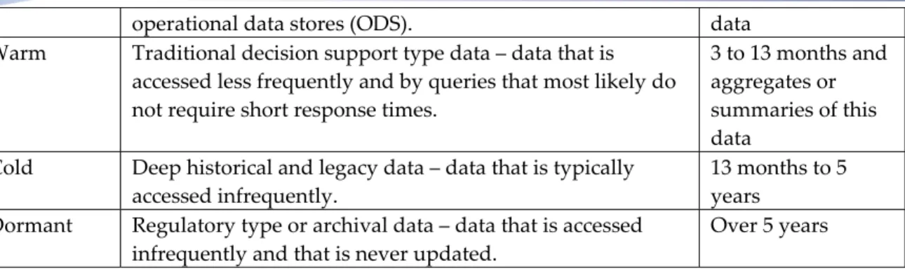
The definition of each data temperature depends on the specific environment, but data temperatures usually fall into fairly common categories. The following chart provides some guidelines for classifying data by temperature:

Data

temperature

Data temperature characteristics Typical data age

Hot Tactical and OLTP type data – current data that is accessed frequently by queries that must have short response times. For example, high volume, small result set point queries in

0 to 3 months and aggregates or summaries of this

2

With the growing popularity but high cost of solid state drives (SSDs), interest in tiered storage is growing. In current IBM Smart Analytics System offerings such as the 5600 and 7700, the SSDs are configured to store temporary table spaces. This paper does not discuss SSDs in more detail.

(5)

operational data stores (ODS). data Warm Traditional decision support type data – data that is

accessed less frequently and by queries that most likely do not require short response times.

3 to 13 months and aggregates or summaries of this data

Cold Deep historical and legacy data – data that is typically accessed infrequently.

13 months to 5 years

Dormant Regulatory type or archival data – data that is accessed infrequently and that is never updated.

Over 5 years

As data ages, the average temperature of the data tends to cool off. There can be temperature fluctuations, or hot spots, as users perform periodic analysis, such as an analysis of the current quarter compared to the same quarter last year. But typically a small proportion of the data in a warehouse is considered hot or warm and 70% to 90% of the data is considered cold or dormant. The following diagram shows a typical

distribution of data across temperature tiers.

Figure 1: Typical distribution of data across temperature tiers

Classification of data into temperature tiers is also affected by the business rules that dictate how your organization moves data between the parts of the data warehouse that support the data of a particular temperature. For example, your organization might always compare the net sales at the end of each fiscal month to the net sales during the same month for the last two years. Such a business rule implies that the definition of warm data should include at least 26 fiscal months.

(6)

Key concepts

This paper refers to the following key concepts:

A database partition is a portion of a database that consists of its own data, indexes, configuration files, and transaction logs. A partitioned database environment is a database installation that supports the distribution of data across database partitions. In an IBM Smart Analytics System data warehouse, there are two types of nodes (physical servers): data nodes, each of which host a fixed number of database partitions, and the administration node, which hosts a single database partition.3

A database partition group is a set of one or more database partitions in a database that have a common distribution map. An IBM Smart Analytics System data warehouse typically contains one database partition group named PDPG that includes all database partitions that store partitioned data (in other words, all database partitions on the data nodes). It also contains one database partition group named SDPG that includes a single database partition. This database partition, which is hosted on the administration node, stores the catalog tables for the database, serves as the coordinator partition, and stores small, non-partitioned tables.

A table space is a storage structure that can contain tables, indexes, large objects, and long data. Table spaces organize data in a database into logical storage groupings that relate to where data is stored on a system. A table space can belong to only a single database partition group.

The two types of table spaces that can be used in IBM Smart Analytics System data warehouses are automatic storage table spaces and database managed space (DMS) table spaces. With automatic storage table spaces, the database manager creates and extends table space containers as needed. With DMS table spaces, the database manager controls the storage space, but unlike with automatic storage table spaces, you specify the table space containers when you create table spaces.

A significant advantage of automatic storage table spaces is that they are much easier to manage than DMS table spaces. However, one disadvantage in a multi-temperature data warehouse is that you cannot distinguish between various types of storage at the table space level: all table spaces must be located on the same type of storage. With DMS table spaces, you can create containers on faster storage for the table spaces that store hot and warm data, and containers on slower storage for the table spaces that store cold and dormant data.

Table partitioning is a data organization schema in which the data in a table is partitioned across multiple storage objects. Each unit of a partitioned table is called a data partition (or sometimes range). In most cases the data partition is defined based on a time dimension,

3

An IBM Smart Analytics System environment also contains other types of nodes, such as a management node, and it can contain standby nodes and application nodes. These types of nodes are not discussed in this paper.

(7)

such as month or quarter. A table that is partitioned into data partitions is called a partitioned table.4

The main benefit of using table partitioning is the ability to attach (“roll in”) and detach (“roll out”) data partitions almost instantaneously. Beginning with DB2 V9.7 databases, the table partitioning feature also provides the ability to partition indexes.

Temperature partitioning is a new term used in this paper that refers to placing one or more sequential data partitions of a partitioned table into a table space based on the temperature of the data. For example, all data partitions that contain hot data are placed into one or more hot table spaces, and all data partitions that contain cold data are placed into one or more cold table spaces. The purpose of temperature partitioning is to limit the number of table spaces that are required for multi-temperature tables.

Cost-based workload management refers to a DB2 workload manager (WLM) configuration that classifies work into different services classes based on the estimated cost of the incoming SQL statements. You can use cost-based workload management if you have different types of storage devices (in other words, faster storage for your hot data and slower storage for your cold data) or a single type of storage device.

Database design for multi-temperature data in an

IBM Smart Analytics System environment

When designing a database for multi-temperature data, the main principle recommended in this paper is to physically separate hot and warm data from cold and dormant data and to isolate the different temperature tiers on different types of storage devices. Place hot and warm data in table spaces that reside on fast storage and cold and dormant data in table spaces that reside on less expensive, slower storage devices. This type of

database design makes all data accessible but optimizes the price-to-performance balance by using lower-cost storage for the data that is rarely accessed or updated.

Physically separate hot and warm data from cold and dormant data by storing data in table spaces based on the temperature of the data. Store hot and warm data on faster storage and store cold and dormant data on slower storage.

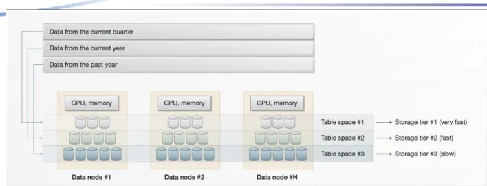
The following diagram demonstrates this design principle. Data from the current quarter is stored in table spaces on fast storage; data from the current year (excluding the current quarter) is stored on fast storage; data from the last year is stored on slower but higher capacity storage.

4_{Do not confuse table partitioning with database partitioning. They are separate data organization schemas. You can use one, both,}

or neither of these schemas. With table partitioning, a table is split into data partitions; with database partitioning, a database is split into database partitions. One or more data partitions can be stored on a single database partition. In this paper, the term partitioned table always refers to a table that is split using table partitioning.

(8)

Figure 2: Sample multi-tier storage setup in a partitioned database environment

By default, IBM Smart Analytics System and InfoSphere Balanced Warehouse offerings include only one type of external storage device. However, you can attach additional storage devices for cold and dormant data. For more information, consult an IBM architect who has experience designing and implementing IBM Smart Analytics System and InfoSphere Balanced Warehouse solutions.

In most IBM Smart Analytics Systems configurations, the database is enabled for automatic storage management and the file systems are set up with the expectation that all table spaces for multipartition data are automatic storage table spaces. For these configurations, keep hot and warm data in automatic storage table spaces.

If you have an InfoSphere Balanced Warehouse configuration or an IBM Smart Analytics System configuration that does not use automatic storage table spaces, place the tables that hold hot and warm data in manually defined DMS table spaces.

After you attach the additional non-default storage to your data nodes for the cold and dormant data, make this storage available to the database by defining separate DMS table spaces on the storage. You cannot define your table spaces for cold and dormant data as automatic storage table spaces because the automatic storage management feature does not allow you to specify table space containers on the additional, non-default storage.

Always store cold and dormant data in DMS table spaces.

Refer to the following recommendations when you are designing tables for multi-temperature data:

• Split tables that hold multi-temperature data into several physically separate tables based on the temperature of the data. For example, if a table contains hot and cold data, split this table into two physically separate tables, one for hot data and the other for cold data. If you need to access data from multiple temperature tiers within a single request, create a view over the union of the data tiers. This technique is described later in this paper.

(9)

o It allows you to implement cost-based workload management.

o It allows you to collect statistics on a table that holds only data of a particular temperature. In general, hot and warm data is much more volatile than cold and dormant data. You might rarely or never need to refresh statistics for your cold and dormant data, which saves time and resources.

• Use table partitioning and organize your data partitions into table spaces based on how frequently you plan to move data from one temperature tier to another. For example, if you plan to move your data from hot to cold storage on a quarterly basis, your table space granularity should be quarterly.

Depending on your scenario, you might choose one of the following methods to manage data in your table spaces:

o Place each data partition into a separate table space.

o Place multiple data partitions into a single table space.

The advantage of the first method is a simpler data model; the advantage of the second method is to limit the number of table spaces in your environment, which can reduce administrative work.

• Define the table spaces for cold and dormant data in the same database partition group as the table spaces for hot and warm tables. The reason for keeping both hot and cold table spaces in the same database partition group is to support collocated joins, which provide better query performance than non-collocated joins.

• When naming table spaces, table space containers, or data partitions for multi-temperature tables, use naming conventions that indicate the date range of the data in the particular table space, table space container, or data partition.

• When naming tables that contain multi-temperature data, use naming conventions that indicate the temperature of the underlying storage.

Isolate hot data from cold data by splitting tables into physically separate tables based on the temperature of the data. Use table partitioning and arrange sequential data partitions in table spaces so that the granularity of each table space matches your schedule for moving data from one temperature tier to another.

Multi-temperature table space and table definition example

The following simple example shows how to create a multi-temperature table that has two temperature tiers (hot and cold) and that is range partitioned by month and

temperature partitioned by quarter. In this example, all data from 2010 is considered hot, and all data from 2009 and 2008 is considered cold.

(10)

If your data warehouse uses automatic storage table spaces, you do not need to specify the path to the default storage paths when you create table spaces, and you can therefore create table spaces for hot data by issuing the following statements:

CREATE TABLESPACE tbsp_2010_q4 IN DATABASE PARTITION GROUP pdpg; ...

CREATE TABLESPACE tbsp_2010_q1 IN DATABASE PARTITION GROUP pdpg;

If your data warehouse does not use automatic storage table spaces, create the table spaces for hot and warm data as DMS table spaces by issuing statements similar to the following examples:

CREATE TABLESPACE tbsp_2010_q4 IN DATABASE PARTITION GROUP pdpg PAGESIZE 16K MANAGED BY DATABASE

USING (FILE '/db2fs/instance_name/NODE000 $N

/database_name/container_2010_q4’ 100G)

ON DBPARTITIONNUMS (1 to 8) EXTENTSIZE 32 PREFETCHSIZE AUTOMATIC OVERHEAD 3.63 TRANSFERRATE 0.07 AUTORESIZE YES;

...

USING (FILE '/db2fs/instance_name/NODE000 $N

/database_name/container_2010_q1’ 100G)

ON DBPARTITIONNUMS (1 to 8) EXTENTSIZE 32 PREFETCHSIZE AUTOMATIC OVERHEAD 3.63 TRANSFERRATE 0.07 AUTORESIZE YES;

In these sample statements, instance_name is the name of the instance and

database_name is the name of the database. Be sure to use the appropriate file path, number of database partitions, extent size, prefetch size, overhead rate, and transfer rate for your configuration. If your multipartition database partition group is not named

pdpg, specify the appropriate name for your configuration.

Assume that in this example, the additional storage is defined on the path

/db2fs_cold/. Whether or not the regular table spaces in your data warehouse use automatic storage, you must define the table spaces on the additional storage as DMS table spaces. Define the table spaces in the same database partition group as the hot data using the following statements as examples:

USING (FILE ‘/db2fs_cold/instance_name/NODE000 $N

/database_name/container_2009_q4’ 100G) ON DBPARTITIONNUMS (1 to 8)

EXTENTSIZE 32 PREFETCHSIZE AUTOMATIC

OVERHEAD 10 TRANSFERRATE 0.1 AUTORESIZE YES; ...

USING (FILE ‘/db2fs_cold/instance_name/NODE000 $N

(11)

For DMS table spaces, it is important to specify appropriate values for the OVERHEAD and TRANSFERRATE arguments. In general, start by specifying the correct values for your storage devices. If you are implementing a cost-based workload manager solution, you might later tune these values only for the table spaces located on the cold storage to force the DB2 optimizer to estimate higher costs for queries that access cold data. For more information, see the section “Managing multi-temperature data with DB2 workload manager (WLM)”.

The following sample statements create separate tables for hot and cold data. The hot table is partitioned into 12 data partitions (one for each month of hot data) and the cold data is partitioned into 24 data partitions (one for each month of cold data). The ellipses

(...) indicate that parts of the statement are not shown.

CREATE TABLE table1_hot (...) PARTITION BY RANGE (col1_date) (

PARTITION part_2010_Jan STARTING (‘2010-01-01’)

ENDING(‘2010-02-01’) EXCLUSIVE IN tbsp_2010_1q, PARTITION part_2010_Feb STARTING (‘2010-02-01’)

ENDING(‘2010-03-01’) EXCLUSIVE IN tbsp_2010_1q, ...

PARTITION part_2010_Dec STARTING (‘2010-12-01’) ENDING(‘2011-01-01’) EXCLUSIVE IN tbsp_2010_4q )

COMPRESS YES DISTRIBUTE BY HASH(...) ORGANIZE BY (...);5

CREATE TABLE table1_cold (...) PARTITION BY RANGE (col1_date) (

PARTITION part_cold_data STARTING MINVALUE IN tbsp_old_data, PARTITION part_2008_Jan STARTING (‘2008-01-01’)

ENDING(‘2008-02-01’) EXCLUSIVE IN tbsp_2008_1q, PARTITION part_2008_Feb STARTING (‘2008-02-01’)

ENDING(‘2008-03-01’) EXCLUSIVE IN tbsp_2008_1q, ...

PARTITION part_2009_Dec STARTING (‘2009-12-01’)

ENDING(‘2010-01-01’) EXCLUSIVE IN tbsp_2009_4q) COMPRESS YES DISTRIBUTE BY HASH(...) ORGANIZE BY (...);

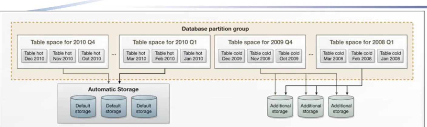
The following diagrams show the sample table space and table definitions created in this example.

5

This sample statement uses the ENDING ... EXCLUSIVE clause to define the range of each data partition. The advantage of using this clause and specifying the first day of the next month is that you do not need to worry about how many days each month contains.

(12)

Figure 3: Sample database design in which the table spaces for hot data are managed using automatic storage

Figure 4: Sample database design in which the table spaces for hot data are DMS table spaces

Creating a view using the UNION ALL clause

If particular users or applications need to access both cold and hot data within the same query, you can create a view over all of the data using the UNION ALL clause, as shown in the following sample statement:

CREATE VIEW union_all AS

SELECT * FROM table1_hot

WHERE col1_date BETWEEN ‘2010-01-01’ AND ‘2010-12-31’ UNION ALL

SELECT * FROM table1_cold

WHERE col1_date BETWEEN ‘2008-01-01’ AND ‘2009-12-31’;

However, whenever possible, access the tables directly rather than using a view because directly accessing tables can provide better performance.

Moving data between temperature tiers

As the data ages and cools off over time, it is important to move it from one temperature tier to another. For example, you can set up a batch job that moves data from one

(13)

temperature tier to another every month or quarter. Because data in different

temperature tiers is stored on separate storage devices, moving the data requires that you physically copy the data from one table space to another.

Before moving data from one temperature tier to another, consider the following points:

• The procedure described here requires that a user or application does not update any data in the portion of the table that is being moved from one table space to another while it is being moved. Generally, users should not be updating data in a table if the data is old enough to be moved to cold storage. However, if it is possible that a user might update the data while it is being moved, lock the table for read-only access while you are moving the data.

• If the data in the table you are moving is compressed, you must complete additional steps. When table compression is active, the cold table does not have an ideal compression dictionary because the automatic dictionary creation (ADC) feature created the compression dictionary at an earlier time, without taking into account a larger sample of the data. There are two methods for ensuring that the compression dictionary for the cold table is effective:

• You can load a subset of data into the cold table, issue the REORG command with the RESETDICTIONARY flag, truncate the table to remove this subset of data, and then move all of the data into the cold table.

• You can issue the REORG command with the RESETDICTIONARY flag after you have moved the data.

For more information about these methods, consult the best practices paper on deep compression that is available from the following site:

http://www.ibm.com/developerworks/data/bestpractices/deepcompression/

The following procedure shows how to move three data partitions (each of which includes one month of data) from a table space that hosts hot data to a table space that hosts cold data. This example is based on the assumption that, every quarter, you move your three oldest months’ worth of data from hot storage to cold storage, and that you have organized your data such that the data for each quarter is stored in a separate table space.

1. Extract the definition of the cold table using the db2look utility, as shown in the following sample command:

db2look –d database_name -e –z table_schema -tw table1_cold;

You must extract the table definition to create a copy of the table in which to store the data you are moving.

2. Create a table space on the cold storage to hold the current hot data that you are moving to the cold table space. Use the following sample statement as a template:

CREATE TABLESPACE tbsp_temp IN DATABASE PARTITION GROUP pdpg PAGESIZE 16K MANAGED BY DATABASE

USING (FILE /db2fs_cold/instance_name/NODE000 $N

(14)

3. For each data partition in the table space, repeat the following steps. In this example, the table space contains three data partitions (one for January, one for February, and one for March), so you must repeat these steps three times.

a. Create a copy of the table in the table space you created on the cold storage. When you create the copy of the table, it should match the table definition you extracted above except that you must provide a new, temporary name for the table, you must create the table in the table space you created, and you must remove the data partition clause from the table definition, as shown in the following example:

CREATE TABLE table1_temp (...) COMPRESS YES DISTRIBUTE BY HASH(...) IN tbsp_temp ORGANIZE BY (...);

b. Insert all records in the data partition that you are currently moving from the hot tier to the cold tier into the new copy of the table. The WHERE clause must contain the same predicates as the definition of the data partition. For example, for the data partition that contains the data from January, the statement might look as follows:

INSERT INTO table1_temp SELECT * FROM table1_hot WHERE col1_data >= ‘2010-01-01’ AND col1_data < ‘2010-02-01’;

To improve the performance of the copy process, you can configure changes to the table not to be logged by specifying the ALTER TABLE statement with the NOT LOGGED INITIALLY parameter before you insert the data into it, as shown in the following statement:

ALTER TABLE table1_temp ACTIVATE NOT LOGGED INITIALLY;

However, this method does not guarantee recoverability if a failure occurs after you move the data, but before your next database backup.

c. If the partitioned table has partitioned indexes, rebuild the indexes

immediately after you have inserted the data into the new table but before you attach this table to the cold table. Rebuilding the indexes at this time improves the availability of the data. The index definitions were extracted when you ran the db2look command. The following sample statement rebuilds an index:

CREATE INDEX index_name ON table1_temp (column_list);

d. Attach the data partition to the cold table using the following statement as an example:

ALTER TABLE table1_cold ATTACH PARTITION part_2010_Jan STARTING (‘2010-01-01’) ENDING(‘2010-01-31’) FROM table1_temp BUILD MISSING INDEXES;

COMMIT;

After you issue this statement, the data is not yet visible to users and applications.

e. Within a single unit of work, make the data you moved visible to users and detach the data partition located on the hot storage. If you have an existing view that takes the union of the hot and cold data, you must also recreate this view within the same unit of work. For more information about creating this

(15)

view, see the section “Creating a view using the UNION ALL clause”. Use the following statements as a model:

SET INTEGRITY FOR table1_cold ALLOW WRITE ACCESS IMMEDIATE CHECKED;

ALTER TABLE table1_hot DETACH PARTITION part_2010_Jan INTO table1_hot_original;

CREATE OR REPLACE VIEW union_all (...)

COMMIT;

During this set of operations the hot and cold tables are briefly locked, but because the ATTACH and DETACH operations are almost instantaneous there should be almost no impact to the users.

f. After the attach operation completes successfully, drop the original detached table in the hot table space:

DROP TABLE table1_hot_original;

4. After you have moved all data partitions from the hot table to the cold table, collect statistics on the cold and hot data using the RUNSTATS command.

5. Drop the original table space and rename the table space you created to the name of the original table space:

DROP TABLESPACE tbsp_2010_q1;

RENAME TABLESPACE tbsp_temp TO tbsp_2010_q1;

6. If you defined any materialized query tables (MQTs) over the multi-temperature data that use the REFRESH DEFERRED option, these MQTs are placed in check pending state after the attach and detach operations complete. Because the underlying data has not changed, you can re-enable these tables for query processing by issuing the SET INTEGRITY ... UNCHECKED statement, as shown in the following example:

SET INTEGRITY FOR mqt_table_name ALL IMMEDIATE UNCHECKED;

7. If you implement cost-based workload management and you use static SQL

packages, rebind the packages. Rebind the packages because the cost of the queries is pre-calculated and stored in the package.

8. If necessary, create a table space and new data partitions on the hot storage device for the data from the upcoming quarter.

Managing multi-temperature data with DB2 workload

manager (WLM)

DB2 workload manager can help you to manage the resources allocated to the queries that access data within each temperature tier. In most cases, a typical goal is to limit the

(16)

number of requests to the cold data so that these queries do not impact the high priority queries and other critical operations that run on the system. Another typical goal is to allocate more resources to the queries that access hot or warm data than to the queries that access cold data.

There are two main approaches with WLM to control the requests that access multi-temperature data: based on connection attributes and based on the estimated cost. After WLM identifies the activity by either its connection attribute or its cost, WLM can control the activity either proactively using concurrency controls and queues, or reactively based on total activity time, processor time, number of rows returned, or other metrics.

The first method for identifying an activity is based on the connection attributes, such as the name of the application, the user ID, the user group, the user role, or special tokens. To apply this approach in a multi-temperature environment, you must be able to identify the users or applications that access data within a particular temperature tier. For

example, if you know that the audit application is doing large table scans on cold data, you can create a separate workload for this application and limit the number of times this application can run concurrently to protect the critical applications that need to access hot data.

If possible, identify applications that access only cold or dormant data and use WLM to limit the concurrency of these applications.

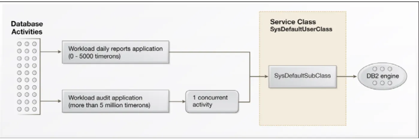
The following diagram shows a WLM configuration in which the daily reports application (a critical application) does not have its concurrency limited, but the audit application (a non-critical application) is limited to a concurrency of one.

Figure 5: Workload management based on connection attributes

However, in most environments it is difficult to control access to data of a certain temperature based only on connection attributes. In these cases, you can instead use cost-based workload management. The main idea of cost-cost-based workload management is to allow trivial queries that finish quickly to complete and to limit the number of concurrent long running complex jobs. To determine if a query is trivial or complex, you can

(17)

optimizer considers the underlying properties of the table spaces, including the overhead and transfer rate, the estimated cost of a query can vary significantly if the data required for the query resides on hot, warm, or cold storage.

To configure the optimizer to assign a higher estimated cost to queries that access cold data on slow storage than to queries that access hot data on fast storage, and to configure WLM to react automatically to a higher estimated query cost, follow these guidelines:

• Start by specifying the correct overhead and transfer rate values for your table spaces. Setting the overhead and transfer rate is important for the DMS table spaces that you create on your slower storage devices. Use the ALTER TABLESPACE statement to set these parameters.

• If specifying accurate values for the overhead and transfer rate does not cause the DB2 optimizer to estimate significantly higher costs for the queries that access cold data, you can later increase these parameters. This technique is described at the end of this section.

• Use a work action set to place DML statements into different service subclasses based on their estimated cost.

• Differentiate the service provided to those service subclasses using activity

concurrency service classes. Do not limit the queries that have a low estimated cost but do limit the queries that have a high estimated cost.

• If you use static SQL packages, rebind the packages after you move the data from a table space in one temperature tier to a table space in another tier. As mentioned earlier in this paper, the reason for rebinding the packages is that the cost of the queries is pre-calculated and stored in the package.

To conserve resources for high-priority queries, use cost-based workload management: set the transfer rate and overhead parameters appropriately for table spaces on slow storage devices and configure WLM to limit the number of concurrent queries that have a high estimated cost.

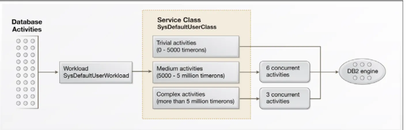
The following diagram shows a WLM configuration in which an unlimited number of trivial queries, six medium queries, and three complex queries are allowed to run concurrently.

(18)

To demonstrate how the type of storage on which data is located can affect the query costs estimated by the DB2 optimizer, we took three queries (trivial, medium, and complex) and had the optimizer estimate the cost of running them against two identical sets of data. In the first case, the data was considered hot, and we set the overhead and transfer rate to low values, to create the effect of storing the data on fast storage. In the second case, the data was considered cold, and we set the overhead and transfer rate to high values, to create the effect of storing the data on slow storage. In both cases we used identical hardware and we did not change any other configuration parameters.

The following table compares the estimates that the optimizer made for the three queries on the two sets of data.

Trivial statement Medium statement Complex statement “Hot” table space

with OVERHEAD 3.63 and

TRANSFERRATE 0.07

11 timerons 194,434 timerons 1,237,854 timerons

“Cold” table space with OVERHEAD 10 and TRANSFERRATE 0.2

30 timerons 263,211 timerons 2,013,610 timerons

As this table shows, the larger the value of OVERHEAD and TRANSFERRATE, the higher the estimated cost of a query. The actual percentage of increase in timeron value depends on many factors.

When you set the overhead and transfer rate values accurately for the type of storage on which your table spaces are located, the DB2 optimizer might not increase the query cost sufficiently for queries that access cold data. As a result, WLM might not categorize these queries into a separate service class. If the queries are not categorized into a

separate service class, you can increase the overhead and transfer rate values for the table spaces on cold storage to make the queries that access the cold data appear to be more expensive than they really are.

You do not need different types of storage to implement a cost-based WLM solution for multi-temperature tables. Even if the table spaces reside on the same physical devices, you can specify a higher value for the OVERHEAD and TRANSFERRATE properties for the table spaces that hold cold data to make the queries that access this data appear more expensive, so that WLM categorizes these queries into a separate service class.

Backup and recovery considerations

When a data warehouse includes large volumes of cold data on inexpensive, slower storage devices, it takes additional time to run a full database backup compared to an environment that contains only fast storage devices. Backup time is directly related to the

(19)

speed of the storage devices. Therefore for warehouses with multi-temperature data, the best practice recommendation is to implement online table space backup. A backup strategy based on table space backups rather than full database backups allows you to take granular backups based on the temperature of the data. For example, you might back up cold and dormant data once a month (synchronized with the movement of data from one temperature tier to another), and you might back up hot and warm data on a daily basis.

Use table space backups rather than full database backups so that you can back up more volatile hot and warm data more frequently and mostly static cold and dormant data less frequently.

Recovery methods depend on the symptoms of the problem that requires you to restore the data (for example, a table space loss, a catalog partition loss, or a database partition loss).

For more information, refer to the best practices paper on backup and recovery that is available from the following site:

(20)

Conclusion

This paper describes how to design, implement, and manage a multi-temperature data warehouse. It also describes the many advantages of multi-temperature data warehouses. They can help reduce your costs by allowing you to use inexpensive storage for the data you rarely need to access. They enable you to keep all of your data accessible within a single data warehouse, even as the volume of historical data grows significantly over time. In addition, with the help of DB2 workload management, you can allocate more resources to high-priority requests for current data than to low-priority requests for extremely old data.

Summary of key recommendations

• Physically separate hot and warm data from cold and dormant data by storing data in table spaces based on the temperature of the data. Store hot and warm data on fast storage and store cold and dormant data on slow storage.

• Always store cold and dormant data in DMS table spaces.

• Isolate hot data from cold data by splitting tables into physically separate tables based on the temperature of the data. Use table partitioning and arrange sequential data partitions in table spaces so that the granularity of each table space matches your schedule for moving data from one temperature tier to another.

• If possible, identify applications that access only cold or dormant data and use WLM to limit the concurrency of these applications.

• To conserve resources for high-priority queries, use cost-based workload

management: set the transfer rate and overhead parameters appropriately for table spaces on slow storage devices and configure WLM to limit the number of

concurrent queries that have a high estimated cost.

• Use table space backups rather than full database backups so that you can back up more volatile hot and warm data more frequently and mostly static cold and dormant data less frequently.

(21)

Contributors

Katherine Kurtz

IBM Smart Analytics System Best Practices

Calisto Zuzarte

STSM, DB2 Query Compiler

Jacques Milman

InfoSphere Technical Leader

Haider Rizvi

STSM, IBM Smart Analytics System

Architect

Subho Chatterjee

Information Management, eXtreme

Analytics Development

Paul Bird

Senior Technical Staff Member, Workload

Manager Architect

(22)

Notices

This information was developed for products and services offered in the U.S.A.

IBM may not offer the products, services, or features discussed in this document in other countries. Consult your local IBM representative for information on the products and services currently available in your area. Any reference to an IBM product, program, or service is not intended to state or imply that only that IBM product, program, or service may be used. Any functionally equivalent product, program, or service that does not infringe any IBM

intellectual property right may be used instead. However, it is the user’s responsibility to evaluate and verify the operation of any non-IBM product, program, or service.

IBM may have patents or pending patent applications covering subject matter described in this document. The furnishing of this document does not grant you any license to these patents. You can send license inquiries, in writing, to:

IBM Director of Licensing IBM Corporation North Castle Drive Armonk, NY 10504-1785 U.S.A.

The following paragraph does not apply to the United Kingdom or any other country where such provisions are inconsistent with local law: INTERNATIONAL BUSINESS MACHINES

CORPORATION PROVIDES THIS PUBLICATION "AS IS" WITHOUT WARRANTY OF ANY KIND, EITHER EXPRESS OR IMPLIED, INCLUDING, BUT NOT LIMITED TO, THE IMPLIED WARRANTIES OF NON-INFRINGEMENT, MERCHANTABILITY OR FITNESS FOR A PARTICULAR PURPOSE. Some states do not allow disclaimer of express or implied warranties in certain transactions, therefore, this statement may not apply to you.

Without limiting the above disclaimers, IBM provides no representations or warranties regarding the accuracy, reliability or serviceability of any information or recommendations provided in this publication, or with respect to any results that may be obtained by the use of the information or observance of any recommendations provided herein. The information contained in this document has not been submitted to any formal IBM test and is distributed AS IS. The use of this information or the implementation of any recommendations or techniques herein is a customer responsibility and depends on the customer’s ability to evaluate and integrate them into the customer’s operational environment. While each item may have been reviewed by IBM for accuracy in a specific situation, there is no guarantee that the same or similar results will be obtained elsewhere. Anyone attempting to adapt these techniques to their own environment do so at their own risk.

This document and the information contained herein may be used solely in connection with the IBM products discussed in this document.

This information could include technical inaccuracies or typographical errors. Changes are periodically made to the information herein; these changes will be incorporated in new editions of the publication. IBM may make improvements and/or changes in the product(s) and/or the program(s) described in this publication at any time without notice.

Any references in this information to non-IBM Web sites are provided for convenience only and do not in any manner serve as an endorsement of those Web sites. The materials at those Web sites are not part of the materials for this IBM product and use of those Web sites is at your own risk.

IBM may use or distribute any of the information you supply in any way it believes appropriate without incurring any obligation to you.

Any performance data contained herein was determined in a controlled environment. Therefore, the results obtained in other operating environments may vary significantly. Some measurements may have been made on development-level systems and there is no guarantee that these measurements will be the same on generally available systems. Furthermore, some measurements may have been estimated through extrapolation. Actual results may vary. Users of this document should verify the applicable data for their specific environment.

(23)

Information concerning non-IBM products was obtained from the suppliers of those products, their published announcements or other publicly available sources. IBM has not tested those products and cannot confirm the accuracy of performance, compatibility or any other claims related to non-IBM products. Questions on the capabilities of non-IBM products should be addressed to the suppliers of those products.

All statements regarding IBM’s future direction or intent are subject to change or withdrawal without notice, and represent goals and objectives only.

This information contains examples of data and reports used in daily business operations. To illustrate them as completely as possible, the examples include the names of individuals, companies, brands, and products. All of these names are fictitious and any similarity to the names and addresses used by an actual business enterprise is entirely coincidental. COPYRIGHT LICENSE:

This information contains sample application programs in source language, which illustrate programming techniques on various operating platforms. You may copy, modify, and distribute these sample programs in any form without payment to IBM, for the purposes of developing, using, marketing or distributing application programs conforming to the application programming interface for the operating platform for which the sample programs are written. These examples have not been thoroughly tested under all conditions. IBM, therefore, cannot guarantee or imply reliability, serviceability, or function of these programs.

Trademarks

IBM, the IBM logo, and ibm.com are trademarks or registered trademarks of International Business Machines Corporation in the United States, other countries, or both. If these and other IBM trademarked terms are marked on their first occurrence in this information with a trademark symbol (® or ™), these symbols indicate U.S. registered or common law

trademarks owned by IBM at the time this information was published. Such trademarks may also be registered or common law trademarks in other countries. A current list of IBM trademarks is available on the Web at “Copyright and trademark information” at www.ibm.com/legal/copytrade.shtml

Windows is a trademark of Microsoft Corporation in the United States, other countries, or both.

UNIX is a registered trademark of The Open Group in the United States and other countries. Linux is a registered trademark of Linus Torvalds in the United States, other countries, or both. Other product and service names might be trademarks of IBM or other companies.