478 IEEE TRANSACTIONS ON COMPUTERS, VOL. 37, NO. 4, APRIL 1988

478 IEEE TRANSACTIONS ON COMPUTERS, VOL. 37, NO. 4, APRIL 1988 D. K. Pradhan and S. M. Reddy, “A fault-tolerant communication

architecture for distributed systems,” IEEE Trans. Comput., vol. C- 31, pp. 863-870, Sept. 1982.

F. P. Preparata and J . Vuillemin, “The cube-connected cycles: A versatile network for parallel computation,” Commun. ACM, vol. 24, pp. 300-309, May 1981.

A. Rucinski and J . L. Pokoski, “Polystructural, reconfigurable, and fault-tolerant computers,” in Proc. 6th Int. Conf. Distributed Comput. Syst., Cambridge, MA, May 1986, pp. 175-182. A. Sengupta, A. Sen, and S. Bandyopadhyay, “On an optimally fault- tolerant multiprocessor network architecture,” IEEE Trans. Com- put., vol. C-36, pp. 619-623, May 1987.

S. Toida, F. J. Meyer, and D. K . Pradhan, “A theorem on the fault- tolerance of a modified de Bruijn network topology,” IEEE Trans. Comput., submitted for publication.

D. K. Pradhan, Fault-Tolerant Computing. Theory and Tech- niques. Englewood Cliffs, NJ: Prentice-Hall, 1986, ch. 6.

Performability Modeling Based on Real Data: A Case Study M. C. HSUEH, R. K. IYER, AND K. S. TRIVEDI

Abstract-This paper describes a measurement-based performability model based on error and resource usage data collected on a multiproces- sor system. A method for identifying the model structure is introduced and the resulting model is validated against real data. Model development from the collection of raw data to the estimation of the expected reward is described. Both normal and error behavior of the system are character- ized. The measured data show that the holding times in key operational and error states are not simple exponentials and that a semi-Markov process is necessary to model the system behavior. A reward function, based on the service rate and the error rate in each state, is then defined in order to estimate the performability of the system and to depict the cost of different types of errors.

Index Terms-Error, measurements, performability, semi-Markov, workload.

I . INTRODUCTION

Analytical models for hardware failure have been extensively investigated in the literature along with performability issues [I]. Although the time for different components to fail is usually assumed to be exponentially distributed, time-dependent failure rates and graceful degradation have been considered [2]. Automatic availability evaluation, assuming a Markov model, is discussed in [3]. A job/task flow-based model is described in [4], where failure occurrence is assumed to be a linear function of the service requests from a job/task flow. As shown in [5], this linear assumption may result in underestimating the effect of the workload, especially when the load is high. A summary of research in software reliability growth models is discussed in [6]; run-time software reliability modeling is discussed in [7].

Although many authors have addressed the modeling issue and have significantly advanced the state of the art, none have addressed Manuscript recevied June 16, 1987; revised November 5 , 1987. This work was supported in part by NASA Grant NAG-1-613, in part by IBM Corporation, and in part by the Joint Services Electronics Program (U.S. Army, U.S. Navy, U.S. Air Force) under Contract N00014-84-C-0149 to R.

K . Iyer and by the Air Force Office of Scientific Research under Contract AFOSR-84-0132 to K. S. Trivedi.

M. C. Hsueh and R. K. Iyer are with the Computer Systems Group, Coordinated Science Laboratory, University of Illinois at Urbana-Champaign, Urbana, IL 61801.

K . S. Trivedi is with the Department of Computer Science, Duke University, Durham, NC 27706.

IEEE Log Number 8719332.

the issue of how to identify the model structure. Furthermore, very few of either the hardware or the software models have been validated with real data. Exceptions are the joint hardwarehoftware model discussed in [8] and a measurement-based model of workload dependent failures discussed in [5]. Both, however, describe only the external behavior of the system and thus do not provide insight into component-level behavior.

In this paper, we build a semi-Markov model to describe the

resource-usage/error/recovery process in a large mainframe system. The model is based on one year of low-level error and performance data collected on a production IBM 3081 system running under the MVS operating system. The 3081 system consisted of dual proces- sors with two multiplexed channel sets. Both the normal and erroneous behavior of the system are modeled. A reward function, based on the service rate and the error rate in each state, is defined in order to estimate the performability of the system, and to depict the cost of different error types and recovery procedures. Two key contributions of this paper are the following.

1) A method for identifying a model-structure for the resource- usage/error/recovery process is introduced and the resulting model is validated against real data.

2) It is shown that a semi-Markov model may better represent system behavior as opposed to a Markov model.

11. RESOURCE USAGE CHARACTERIZATION In this section, we identify a state-transition model to describe the variation in system activity. System activity was characterized by measuring a number of resource usage parameters. A statistical clustering technique was then employed to identify a small number of representative states.

The resource usage data were collected by sampling, at predeter- mined intervals, a number of resource usage meters, using the IBM MVS/370 system resource measurement facility (RMF). A sample- time of 500 ms was used in this study. Four different resource usage measures were used.

CPU - fraction of the measured interval for which the CPU is executing instructions,

CHB - fraction of the measured interval for which the channel was busy and the CPU was in the wait state (this parameter is commonly used to measure the degree of contention in a system)

S I 0 - number of successful Start I/O and Resume I/O instruc- tions issued to the channel

DASD - number of requests serviced on the direct access storage devices.

At any interval of time, the measured workload is represented by a point in a four-dimensional space, (CPU, CHB, SIO, DASD). Statistical cluster analysis is used to divide the workload into similar classes according to a predefined criterion. This allows us to concisely describe the dynamics of system behavior and extract a structure that already exists in the workload data. I

Each cluster (defined by its centroid) is then used to depict a system state and, a state-transition diagram (consisting of intercluster transition probabilities and cluster sojourn times) is developed. A k- means clustering algorithm [lo] is used for cluster analysis. The algorithm partitions an N-dimensional population into k sets on the basis of a sample. The k nonempty clusters sought, CI, Cz,

. . .

,

Ck,

are such that the sum of the squares of the Euclidean distances of the cluster members from their centroids, E:=, C x , E ~ , Ilx, -

%,\I2,

is minimized, where 2, is the centroid of cluster C,.

Two types of workload clusters were formed. In the first case, CPU and CHB were selected to be the workload variables. This combination was found to best describe the CPU-bound load (nearly

’

Similar clustering techniques are also used for workload characterization in [9].

IEEE TRANSACTIONS ON COMPUTERS, VOL. 3 1 , NO. 4 , APRIL 1988

479

TABLE I

CHARACTERISTICS OF CPU-BOUND WORKLOAD CLUSTERS

I

Cluster

11

% o f

I

Mean

I

Mean

11

Stddev

1

Stddev

I

id

I(

obs

I

of CPU

I

O f C H B

II

of CPU

I

of CHB W . 7.44 I 0.0981 I 0.1072 11 0.0462 1 0.0436

R 2 of CHB = 0.8095 overall R Z = 0.9604

R 2 : the square of correlation eoe5cient

to W O to W O from W O I \ 0.20 from W O o?sl 0.037 0.162 to W O from W O to W O from W O Fig. 1. State-transition diagram of CPU-bound load.

60 percent of the observations have a CPU usage greater than 0.72). In the second case, the clusters were formed considering S I 0 and DASD as the workload variables. This combination was found to best describe the I/O workload. In this paper, only the results for CPU- bound load clusters are presented. Details of U0 activity can be found in [ I l l . Table I shows the results of the clustering operation. The table shows that about 36 percent of the time the CPU was heavily loaded (0.96) and almost 76 percent of the time the CPU load was above 0.5. Since the measured system consisted of two processors, we may say that 76 percent of the time at least one of the processors is busy. A state-transition diagram of CPU-bounded load activity is shown in Fig. 1. Note that a null state WO has been incorporated to represent the state of the system during the nonmeasured period. The time spent in the null state was assumed to be zero. The transition probability from state i to state j , p i j , was estimated from the measured data using

observed number of transitions from state i to state j observed number of transitions from state i In the next section, the characterization of the errors and the recovery process is discussed. The appropriate error and recovery states are identified for subsequent use in developing an overall model.

p . . = '

111. ERROR AND RECOVERY CHARACTERIZATION The IBM system has built-in error detection facilities and there are many provisions for hardware and software initiated recovery through retry and redundancy. The error and recovery data are automatically logged by the operating system as the errors occur. On

the occurrence of an error, the operating system creates a time- stamped record describing the error, the state of the machine at the time of the error, and the result of the hardware and/or software attempts to recover from the error. Details of this logging mechanism are described in [12]. Due to the manner in which errors are detected and reported in a computer system, it is possible that a single fault may manifest itself as more than one error, depending on the activity at the time of the error. The different manifestations may not all be identical [13]. The system recovery usually treats these errors as isolated incidents. Thus, the raw data can be biased by error records relating to the same problem. In order to address this problem, two levels of data reduction were performed. First, a coalescing algorithm described in [5] was used to analyze the data and merge observations which occur in rapid succession and relate to the same problem. Next, a reduction technique described in [13] to automati- cally group records most likely to have a common cause was used. By using these two methods, the errors were classified into five different classes. These classes are called error events since they may contain more than one error and are explained below.

CPU : Errors which affect the normal operation of the CPU; may originate in the CPU, in the main memory, or in a channel

CHAN : Channel errors (the great majority are recovered) DASD : Disk errors, recoverable (by data correction, hardware

instruction retry or software instruction retry), and nonrecoverable disk

SWE : Software incidents due to invalid supervisor calls, program checks, and other software exception condi- tions

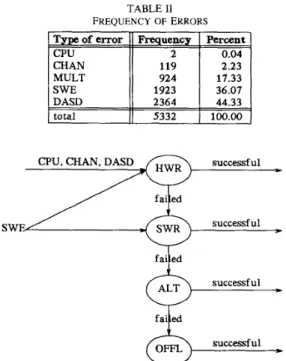
Multiple errors affecting more than one type of compo- nent (i.e., involving more than one of the above). Table I1 lists the frequencies of different types of errors. Notice that about 17 percent of errors are classified as multiple errors (MULT). A MULT error is mostly due to a single cause but the fault has nonidentical manifestations, provoked by different types of system activity. Since the manifestations are nonidentical, recovery may be complex and, hence, can (as will be seen latter) impose considerable overhead on the system.

The recovery procedures were divided into four categories based on recovery cost, which was measured in terms of the system overhead required to handle an error. The lowest level (hardware recovery) involves the use of an error correction code (ECC) or hardware instruction retry and has minimal overhead. If hardware recovery is not possible (or unsuccessful), software-controlled recovery is invoked. This could be simple, e.g., terminating the current program or task in control, or complex, e.g., invoking specially designed recovery routine(s) to handle the problem. The third level, alternative (ALT), involves transferring the tasks to functioning processor(s) when one of the processors experiences an unrecoverable error. If no on-line recovery is possible, the system is brought down for off-line (OFFL) repair. Fig. 2 shows a flow chart of the recovery process. The time spent in each recovery state was taken to be constant, since each recovery type except OFFL requires almost constant overhead.

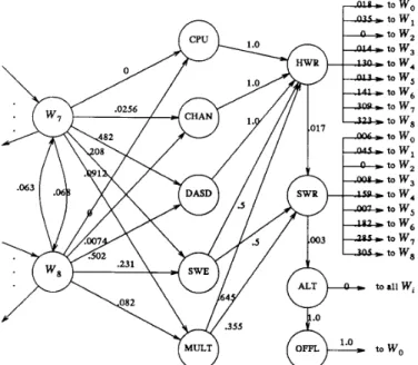
IV. RESOURCE-USAGE/ERROR/RECOVERY MODEL In this section, we combine the separate workload, error, and recovery models developed into a single model shown in Fig. 3. The MULT :

Hardware recovery involves hardware instruction retry or ECC correc- tion. The maximum number of retries is predetermined. Each CPU has a 26- ns machine cycle time and the disk seek time is about 25 ms. We estimate a worst case hardware recovery cost of 0.5 s, i.e., incorporating 20 IiO retries: ten through the original U0 path and another ten through an alternative 110 path if the alternative is available. This, of course, overestimates the cost of hardware retry used for the CPU errors. Similarly, the worst case software recovery time was estimated to be 1 s. The ALT state was not evaluated since it did not occur in the data. For OFFL, the time was calculated to be 1 h based on our experience and through discussion with maintenance engineers.

480 IEEE TRANSACTIONS ON COMPUTERS, VOL. 37. NO. 4, APRIL 1988

TABLE I1 FREQUENCY OF ERRORS ~ s p e of error

11

~ r e q uency

I

Percent

CPU 2 1 0.04

DASD 44.33

total

1)

5332

1

100.00

/

failed

sw

Fig. 2. Flow chart of recovery processes.

null state WO is not shown in this diagram. The model has three different classes of states: normal operation states ( S N ) , error states ( S E ) , and recovery states ( S R ) . Under normal conditions, the system makes transitions from one workload state to another. The occur- rence of an error results in a transition to one of the error states. The system then goes into one or more recovery modes after which, with a high probability, it returns to one of the “good” workload states3 The state transition diagram shows that nearly 98.3 percent of hardware recovery requests and 99.7 percent of software recovery requests are successful. Thus, the error detection, fault isolation, and on-line recovery mechanisms allow the measured system to handle an error efficiently and effectively. In less than 1 percent of the cases is the system not able to recover.

One state which needs further elaboration is the MULT state. Recall that a MULT state denotes a multiple error event affecting more than one component type. Fig. 4 shows the state-transition diagram of a MULT error event, i.e., the transition diagram given a MULT error. The model quantifies the interactions between the different components in a multiple error occurrence. From the diagram, it is seen that in about 65 percent of the cases, a multiple error starts as a software error (SWE) and in 32 percent of the cases it starts as a disk error (DASD). Given that a disk error has occurred, there is nearly a 30 percent chance that a software error will follow. It is also interesting to note that there is a 64 percent chance that one software error will be followed by another different software error. A . Distributions f o r Workload and Error States

Table I11 shows the characteristics of both the workload and error states in terms of their waiting times. An examination of the mean and standard deviation of the waiting times indicates that not all waiting times are simple exponentials. This is particularly pronounced for the error states. Fig. 5(a) and (b) shows the densities of waiting time for W, state and also the specific holding time to the SWE error state. The waiting time for state i is the time that the process spends in state

i before making a transition to any other state. The holding time for a

transition from state i to state j is the time that the process spends in state i before making a transition to state j [14]. This is the same as the distribution of a one-step transition from state i to j . The distributions in Fig. 5 are fitted to phase-type exponential density functions [15] and tested by using the Kolmogorov-Smirnov test at a 0.01 significance level.

B. Error Duration Distributions

Recall that an error event can involve more than one error since errors frequently occur in bursts. During an error burst, the system goes into an error+recovery cycle until the error condition disap- p e a r ~ . ~ In such cases, we measure the duration of an error event as the time difference between the first detected error and the last detected error caused by the same event. The duration of an error event can be used to measure the severity of the error. Since each recovery type takes approximately a constant amount of time, the loss of work can be approximated by the error rate in this period. In Section VI, we use this information to build a reward model for the system. Fig. 6 shows examples of error duration densities for two different types of errors, SWE and MULT.

In summary, we have developed a state-transition model which describes the normal and error behavior of the system. A key characteristic of the model is that the waiting time in some of the workload states and in most error states cannot be modeled as simple exponentials. Furthermore, the folding times from a given workload state to different error states are dependent on the destinations. Thus, the overall system is modeled as a complex irreducible semi-Markov process.

V. MODEL BEHAVIOR ANALYSIS

Now that we have an overall model, we show the usage of this model to predict key system characteristics. The mean time between different types of errors is evaluated along with model characteristics, such as the occupancy probabilities of key normal and error states. A . General Characteristics

By solving the semi-Markov model, we find that the modeled system made a transition every 9 min and 8 s, on average. In comparing this to the mean time between errors (MTBE) listed in Table IV, it is clear that most often the transitions are from one normal state to another. The table also shows that a DASD error was detected almost every 52 min (0.87 h) while a software error was detected every 1 h and 45 min. Most of the DASD errors (95 percent) were recovered through hardware recovery (i.e., hardware instruc- tion retry or ECC), thus resulting in negligible overhead. Table IV also lists the mean recurrence time for recovery states. Thus, the on- line hardware recovery routine is invoked once every 0.62 h, while the software recovery occurs every 2.57 h. By using an estimated time for each hardware recovery and comparing the results to the recovery overhead, we estimate that the cost of hardware recovery is only 0.02 percent of total computation time. The mean recurrence time of the alternative recovery routine was not estimated, due to lack of data, i.e., this event seldom occurred.

B. Summary Model Probabilities

Since the process is modeled as an irreducible semi-Markov process, we can evaluate the following steady state parameters [14]: 1) occupancy probability (+,)-the probability that the process occupies state j ,

2) conditional entrance probability (.lr,)-given that the process is now making a transition, the probability that the transition is to state 3) entrance rate (e,)-the rate at which the process enters state; at any time instance (e, = r,/?, where 7‘ is the mean time between transitions), and

j ,

Note that the transition probabilities from W, to W , are different from those in Fig. 1 where error states were not considered in computing the transition probabilities.

This is typical of many systems (e.g., see [8]). The final recovery usually occurs because the conditions which triggered the error disappear due to change in system activity.

48 1

IEEE TRANSACTIONS ON COMPUTERS, VOL. 37, NO. 4, APRIL 1988

entry to .32 0.0

U

O 2o 40 k 0 a t i o n % i n u 3 120 140 (a) exit from /' MULT

Fig. 4. State-transition diagram of a given multiple error ( MUL T )

T A B L E 111

ERROR STATES

CHARACTERISTICS OF WAITING TIME (SECONDS) IN WORKLOAD AND

* statistically insigni5cant

(b)

Fig. 5 . Waiting and holding time densities. (a) Waiting time density for W,. (b) Holding time density from W, to S W E state.

f ( t ) = 0.041181 e4'0445181

Prob.0.5 - - - _ _ _ _ _ _ _ _ _ _ _ _ _ _ _ _ _ _ _ _ _ _ _ _ _ _ _ _ _ _ _ _ _ _ _ - - - -

+

0.0002704 e-0'00360751

I

(b)

Waiting time density for M U L T .

482

Error states

CPU

I

CHAN

I

SWE

I

DASD

I

MULT

-

I

26.88

I

1.75

I

0 .8 7

I

4.62

IEEE TRANSACTIONS ON COMPUTERS, VOL. 37. NO. 4. APRIL 1988

Recovery s t a t e s HWR

I

SWR

I

ALT

I

OFFL

0. 62

I

2.57

I

-

I

651.37 Error states

CPU

I

CHAN

I

SWE

I DASD

I

MULT

-

I

26.88

I

1.75

I

0 .8 7

I

4.62 Recovery s t a t e s HWR

I

SWR

I

ALT

I

OFFL 0.6’

’

’

C 7 I - I 6 5 ’ 77 Measure a 0

T

e

0”

Normal state WO W,

w,

w,

w,

w,

w6

w,

w8

0.0625 0.0008 0.0136 0.1258 0.0054 0.1639 0.2255 0.3398 0.0257 0.0264 0.0014 0.0104 0.0559 0.0047 0.0635 0.1125 0.1127 O.oooo5 o.oooo5 - o.ooo02 0.0001 o.oooo1 0.00012 0.00021 0.00021 5.78 5.62 102.56 14.32 2.65 31.38 2.33 1.32 1.32

Error state

4) mean recurrence time @,)-mean time between successive entries into state j .

The model characteristics are summarized in Table V. A dashed line in this table indicates a negligible value (statistically insignifi- cant). Table V(a) shows the normal system behavior. For example, given that a transition occurs, the system is most likely to go to states

W, or W,. This is also reflected in the respective entrance rates and

Recovery state

occupancy probabilities for the mentioned states. From the occu- pancy probabilities (+) we see that almost 34 percent of the time the CPU load is as high as 0.96 ( W,); 39 percent of the time, the CPU is moderately loaded ( W ,

+

W,). Table V(b) shows the error behavior of the system. The table shows that about 30 percent of the transitions are to an error state (obtained by summing all the a’s for all the error states). The DASD errors have the highest entrance probability. For the data shown in the table, it can be estimated that an error is detected, on the average, every 30 min. Of course, over 98 percent of these errors incur negligible overhead.

An interesting characteristic of the multiple errors is also seen in Table V(b). Although the entrance probability of a MULT error is lower than that for SWE, its occupancy probability is higher. This is due to the fact that a MULT error event has a longer mean waiting time as compared to SWE error events (293 s versus 41 s). C. Model Validation

Even though our model is developed from real data, it needs to be validated since the model identification process, e.g., the workload clustering, allows us to only approximate the real system behavior. In order to evaluate the validity of the model, three measures evaluated via the model were compared to direct calculations from the actual data. Table VI shows the comparison of the occupancy probabilities for key normal states (occupancy probability greater than 0.1) and for one key error state (DASD). The table also shows the comparison for the mean recurrence time (0) of the SWE error event and for its standard deviation (Std). It can be seen that all the predicted values

Measure

77

e

0

_n

The “actual” values are calculated from observed data. For example, total time that the system was observed to be in state i.

length of the observation period

a, =

CPU CHAN SWE DASD MULT HWR SWR ALT OFFL

- O.oooO5 0.0066 0.0383 0.0179 0.00022 0.00011 - - 0.0055 0.0850 0.1692 0.0322 0.2379 0.0572 - 0.00023 - O.oooO1 0.00016 0.00032 0.00006 0.00045 0.00011 - - 26.88 1.75 0.87 4.62 0.62 2.57 - 651.37 ** in hours (b)

’

s e c 2 TABLE VI

COMPARISON OF @, 8 , AND STANDARD DEVIATION

I II

- O.OOO8 0.0031 0 . 0 2 4 2 0.0156 0.0156 0.022 0 .03 3 a1

E : the absolute error. I Model - Actual I

are around 3 percent or less, indicating that the proposed semi- Markov model is an accurate estimator of the real system behavior. This also provides support for the model structure identification method employed in this paper.

D. Markov Versus Semi-Markov

This section investigates the significance of using a semi-Markov model to describe the overall resource-usage/error/recovery process. It has been argued that since errors only occur infrequently (i.e., h is small), a Markov model may well approximate the real behavior. Clearly, if only the first moments, e.g., MTBE, are of interest, the Markov model provides adequate information. If the distributions (e.g., the time to error distribution) or higher moments are of interest, the Markov model may be inadequate. Thus, although our evidence shows that the semi-Markov process is a better model, i.e., more closely approximates the data from the measured system, it is reasonable to ask what deviations occur if a Markov process is assumed. In order to answer this question, we use a Markov model to describe our system and compare the results to those obtained through the more realistic semi-Markov model.

We compared the two by calculating two steady-state parameters. The first is the complementary distribution of the time to error [referred to as R(t)] for different error types. The second is the standard deviation of R( t ) . The results for the SWE state are shown in Table VII. It is clear that the Markov model overestimates the R(t) in the early life (for low time to error probabilities) and underestimates

R(t) for high time to error probabilities. The standard deviation is also considerably underestimated by the Markov model thus casting doubts on the validity of using MTBE estimates themselves.

IEEE TRANSACTIONS ON COMPUTERS, VOL. 31, NO. 4, APRIL 1988 R(t) 483 Std (mins) Markov 1.00 0.71 0.50 0.35 0.25 0.17 0.12 0.09 25.13 TABLE VI11

REWARD RATES FOR ERROR STATES

State

11

DASD

1

SWE

I

CHAN

I

MULT

11

0.5708

I

0.2736

I

0.9946

I

0.2777

ri

In summary, our measurements show that using a Markov model is optimistic in the short run and pessimistic in the long run. The underestimation of the standard deviation of R ( t ) is also a serious problem because it calls into question the representativeness of the MTBE estimates.

VI. PERFORMABILITY ANALYSIS

In this section, we use the workload/error/recovery model to evaluate the performability of the system. Reward functions are used to depict the performance degradation due to errors and also due to different types of recovery procedures. Since the recovery overhead for each recovery state in the modeled system is approximately constant, the total recovery overhead for each error event and thus the reward depends on the error rate during that event. Thus, the higher the error rate during an error event, the higher is the recovery overhead and, hence lower the reward. On this basis we define a reward the reward rate, r, (per unit time) for each state of the model as follows:

st

i f i E S , U

sE

r,=

ts

S , + e,

if i E SR

where the s, and e, are the service rate and the error rate in state i, respectively. Thus, one unit of reward is given for each unit of time when the process stays in the good states S,. The penalty paid depends on the number of errors generated by an error event. With an increasing number of errors, the penalty per unit time increases, and accordingly, the reward rate decreases. Zero reward is assigned to recovery states. Based on this proposal, reward rates for the error states are as shown in Table VIII.

The reward rate of the modeled system at time t is a random variable X ( t ) , which is defined as

1 r,

0 otherwise.

process is in state i E SN process is in state i E SE

Therefore, the expected reward rate E[X(t)] can be evaluated from E[X(t)] = C p ( t ) r , . The cumulative reward by time t is Y(t) = .(;

X ( o ) do, and the expected cumulative reward is given by [16]

where p l ( t ) is the probability of being in state i at time t. In order to evaluatep,(t) and hence other measures, we convert the semi-Markov process into a Markov process using the method of stages [15], 1171. The state probability vector P*(t) = (.

. .

, p i ( t ) ,

. .

.) of the Markov process can be derived from P*(t) = P*(O)e@, where P*(O) = (1 , 0,

. . .

, 0) and Q is transition rate matrix of the Markov process [ 141. In order to study the performance degradation due to different

types of errors, the irreducible semi-Markov process was trans- formed by considering the OFFL (off-line repair) state as the absorbing state. The expected reward calculated with this assumption indeed reflects the true performability until system failure. Next, for evaluating the impact of different error events we first observe that often these events have significant error duration time (e.g., MULT state has an mean error duration of 5 min with a standard deviation of 4 min). Since the majority ofjobs last less than a few minutes, as far as a user program is concerned, an entry into a long duration error state is similar to entering an absorption state with ri

>

0. Thus, the impact of the MULT can be evaluated by making it into an absorption state with

ri

>

0. A similar analysis can be performed for other error states.

In our analysis, we first make the OFFL state the absorbing state. This gives the expected performance until an off-line failure. Then we evaluate three other cases.

a) OFFL case (OFFL),

b) MULT and OFFL case (MULT), c) SWE, MULT and OFFL case (SWE), and d) DASD, MULT and OFFL case (DASD).

Case a) gives the overall performability of the system assuming that OFFL (off-line repair) is the absorbing state, i.e., the impact of all other error events are taken into account. This gives both the transient and steady-state performability of the system. Next we assume in case b) that both MULT and OFFL are absorbing. The difference between a) and b) approximates the expected performance loss due to possible entry into a long duration MULT state. Similarly, the difference between a) and c) provides an estimate of loss of performance due to entry into an SWE state. In the long term, of course, each will reach a steady-state value. The above analyses were performed on the resulting Markov reward of the system using SHARPE (the symbolic hierarchical automated reliability and performance evaluator)

’

devel- oped at Duke University.

The curves of Fig. 7 show the expected reward rate at time t , E [ X ( t ) ] , for these four cases. The evaluations of the cumulative reward, E [ Y ( t ) ] , are discussed in [ l l ] . In practical terms, the differences provide an estimate of the loss in reward due to various error types assuming that the jobs are initiated when the system is fully operational. As an example, in Fig. 7, we find that the SWE event degrades system effectiveness considerably more than the DASD event. This is because the reward rate of SWE error is lower than DASD error even though the error probability of DASD event is higher than of SWE event.

VII. CONCLUSION

In this study, we have proposed a methodology to construct a model of resource usage, error, and recovery in a computer system, using real data from a production system. The semi-Markov model obtained is capable of reflecting both the normal and error behavior of our measured system. The errors are classified into various types, based on the components involved. Both hardware and software errors are considered, and the interaction between the system An alternative approach, the performance loss (PL) based on the steady- state occupancy probabilities, was suggested by one of the referees. PL, = @,(I - r , )

+

C r E S R is the probability of visiting a recovery state r after an error state i.

’

S HA R PE is a modeling tool. It provides several model types ranging from reliability block diagrams to complex semi-Markov models [ 171.

484

I \ 1 nm. - - - MULT 1.0

..

L

t

I

0.01-. ”’ ’ ”’ . ’ ’ ’ . . . ’ _ .

. * . . . I

0 5 10 15 20 25 30 35 Expected reward rate, E [ X ( t ) ] .

Minutes (b) Fig. 7.

components (hardware and software) is reflected in a multiple error model. The proposed reward measure allows us to predict the performability of the system based on the service and error rates. It is suggested that other production systems be similarly analyzed so that a body of realistic data on computer error and recovery models is available.

ACKNOWLEDGMENT

The authors would like to thank J . Gerardi and the members of Reliability, Availability and Serviceability Group at IBM-Poughkeep- sie for access to the data and for their valuable comments and suggestions. Thanks are also due to Dr. W. C. Carter f o r valuable discussions during the initial phase of this work. We also thank L. T. Young and P. Duba for their careful proofreading of the draft of this manuscript. Finally, we thank the referees for their constructive comments which were extremely valuable in revising the paper.

REFERENCES

J. F. Meyer, “Closed-form solutions of performability,” IEEE Trans. Comput., pp. 648-657, July 1982.

R. M. Geist, M. Smotherman, K . S . Trivedi, and J. Bechta Dugan, “The reliability of life critical systems,” Acta Informatica, vol. 23, A. Goyal, W. C. Carter, E. de Souza e Silva, S . S . Lavenberg, and K.

S . Trivedi, “The system availability estimator,” in Proc. 16th In?. Symp. Fault-Tolerant Comput., Vienna, Austria, July 1986. 0. Schoen, “On a class of integrated performanceireliability models based on queuing networks,” in Proc. 16th Int. Symp. Fault- Tolerant Comput., Vienna, Austria, July 1 4 , 1986, pp. 90-95. R. K. Iyer, D. J. Rossetti, and M. C. Hsueh, “Measurement and modeling of computer reliability as affected by system activity,” A C M Trans. Comput. Syst.. vol. 4, pp. 214-237, Aug. 1986.

B. Littlewood, “Theories of software reliability: How good are they and how can they be improved?” IEEE Trans. Software Eng., vol. SE-6, pp. 489-500, Sept. 1980.

M. C. Hsueh and R. K . Iyer, “A measurement-based model of software reliability in a production environment,” in Proc. 11th Annu. In?. Comput. Software Appl. Conf., Tokyo, Japan, Oct. 7-9, X. Castillo, “A compatible hardware/software reliability prediction model,” Ph.D. dissertation, Carnegie-Mellon Univ., July 1981. pp. 621-642, 1986.

1987, pp. 354-360.

IEEE TRANSACTIONS ON COMPUTERS, VOL. 37, NO. 4, APRIL 1988 D. Ferrari, G . Serazzi, and A. Zeigner, Measurement and Tuning of Computer Systems.

H. Spath, Cluster Anabsis Algorithms. West Sussex, England: Ellis Horwood, 1980.

M. C. Hsueh, “Measurement-based reliabilityiperformability models,’’ Ph.D. dissertation, Dep. Comput. Sci., Univ. Illinois at Urbana-Champaign, Aug. 1987.

IBM Corp. Environmental Record Editing & Printing Program, IBM Corp., 1984.

R. K . Iyer, L. T. Young, and V. Sridhar, “Recognition of error symptoms in large systems,” in Proc. I986 IEEE-ACM Fall Joint Comput. Conf., Dallas, TX, Nov. 2-6, 1986, pp. 797-806. R. A. Howard, Dynamic Probabilistic Systems. New York: Wiley, 1971.

K . S . Trivedi, Probability and Statistics with Reliability, Queuing, and Cornputer Science Applications. Englewood Cliffs, NJ: Pren- tice-Hall, 1982.

R. M. Smith and K. S . Trivedi, “A performability analysis of two multiprocessor systems,” in Proc. 17th Int. Symp. Fault-Tolerant Comput., Pittsburgh, PA, July 6-8, 1987, pp. 224-229.

R. A. Sahner and K. S . Trivedi, “Reliability modeling using SHARPE,” IEEE Trans. Reliability, pp. 186-193, June 1987.

Englewood Cliffs, NJ: Prenctice-Hall, 1981.

Distributed and Fault-Tolerant Computation for Retrieval Tasks U s i n g Distributed Associative Memories

JOIS MALATHI CHAR, VLADIMIR CHERKASSKY,

HARRY WECHSLER, AND GEORGE LEE ZIMMERMAN

Abstract-We suggest the distributed associative memory (DAM) model for distributed and fault-tolerant computation as related to retrieval tasks. The fault tolerance is with respect to noise in the input key data and/or local and global failures in the memory itself. We have developed working models for fault-tolerant image recognition and database information retrieval backed up by experimental results which show the feasibility of such an approach.

Index Terms-Database retrieval, distributed associative memory (DAM), distributed computation, fault tolerance, neural networks, recognition.

I. INTRODUCTION

Artificial Intelligence (AI) deals with the types of problem solving and decision making that humans continuously face in dealing with the world. Such activity involves by its very nature complexity, uncertainty, and ambiguity, all o f which can distort the phenomena being analyzed. However, following the human example, any corresponding computer system should process information such that the results are invariant to the vagaries of the data acquisition process. Furthermore, one would expect such computer systems to be fault tolerant, i.e., to display robustness, if and when some of their hardware were to fail. We suggest in this paper how a particular type Manuscript received April 15, 1987; revised October 15, 1987. This work was supported in part by the Graduate School at the University of Minnesota (J. M. Char and V. Cherkassky). by the National Science Foundation under Grant EET-8713563 to H. Wechsler, and by the Microelectronics and Information Science Center (MEIS) of the University of Minnesota (G. L. Zimmerman).

J. M . Char is with the Department of Computer Science, University of Minnesota, Minneapolis, MN 55455

V. Cherkassky, H. Wechsler, and G. L. Zimmerman are with the Department of Electrical Engineering, University of Minnesota, Minneapolis, MN 55455

IEEE Log Number 8719338. 0018-9340/88/0400-0484$01.00

0

1988 IEEE