Vol. 7, No. 1, 2014, 1-21
ISSN 1307-5543 – www.ejpam.com
On Multivariate Time Series Model Selection Involving Many
Candidate VAR Models
Xindong Zhao
1, Guoqi Qian
2,∗1Institute of Econometrics, Huaqiao University, Xiamen, China
2Department of Mathematics and Statistics, University of Melbourne, Melbourne, Australia
Abstract. Vector autoregressive (VAR) models are important and useful for modelling multivariate time series. An appropriate VAR model is often required for such modelling for given data, for which several model selection criteria such as AIC, AICc, BIC and HQ are available. However, when the number of candidate models available for selection is extremely large, which is not uncommon in practice, performing an exhaustive VAR model selection using any of the above criteria would become computationally infeasible. To overcome this difficulty, we have developed a Markov chain Monte Carlo method based on Gibbs sampler. It is shown that the developed method identifies the optimal VAR model with high probability and efficiency. To illustrate and verify the method, we also present a simulation study and an example on modelling the data of China’s money supply and consumer price index (CPI).
2010 Mathematics Subject Classifications: 62M10, 65C40, 65C60
Key Words and Phrases: Vector autoregressive (VAR) models, Gibbs sampler, Multivariate time series model selection
1. Introduction
VAR modelling is a major area of interest in multivariate time series analysis. Once the approach of VAR modelling is adopted for a data set given, choosing an appropriate VAR model for best modelling would become the next important task. Information-theoretic cri-teria such as AIC and BIC are general and effective model selection methods for measuring the “goodness” of the candidate models. As shown in [8], the information-theoretic crite-ria provide better model selection performance than many other model selection methods. Moreover, Granger, King and White[15]noted that the information-theoretic criteria involve fewer limitations than hypothesis test-based methods, and hence have become popular with model selection practitioners. By comparing every possible candidate model with each other in terms of their respective criterion values, the model with the lowest criterion value can be
∗Corresponding author.
Email addresses:[email protected](X. Zhao),[email protected](G. Qian)
considered as the best estimate of the unknown true model. However, difficulty may arise in VAR model selection when the number of the candidate models is extremely large. Specifi-cally, assuming that some of the coefficients in the VAR system are actually equal zero (i.e. zero restricted) in the true model, then there would be 2pq2+q candidate VAR models for us to decide which of them is the true one. Here p is the order of autoregression andq is the dimension of data at each time point. Even when porqis small, sayp=3 andq=3, which is very possible for multivariate time series, there would be as many as 230candidate models. Clearly, it is computationally infeasible to conduct model selection by comparing every pos-sible candidate model with each other in terms of their respective model selection criterion values.
Fortunately, with the availability of powerful computers and recently developed intensive statistical computing technology we are able to develop an efficient model selection proce-dure in this paper, by which we can find the best model estimate with high probability and efficiency, and without a need to compare all candidate models one by one. The key idea in our procedure is to first establish a probability distribution induced from the criterion values of all candidate models, and then generate samples of candidate models from this distribution using Gibbs sampler, a special algorithm of the Markov chain Monte Carlo method (MCMC). By our procedure, the model that has the lowest criterion value will tend to appear among the earliest and the most frequent in the sample if the number of the models being generated is large enough. Since the generated sample usually has a size of only a small fraction of that of all candidate models, the proposed algorithm is computationally feasible and efficient.
The aim of this paper is not to propose another VAR model selection criterion. Rather we focus on the aforementioned computing issue of VAR model selection that is largely ignored in literature but needs to be addressed when there are very many candidate models available for selection. We still need to employ an existent criterion such as AIC and BIC in our model selection procedure.
The paper is organized as follows. Section 2 introduces the basics of VAR modelling. Sec-tion 3 describes several commonly used model selecSec-tion criteria and the computing difficulty in VAR model selection. Section 4 provides details of the proposed model selection procedure and empirical rules on how to perform model selection in practice. Then in section 5 we provide a simulation study and complete the analysis of model selection for China’s money supply and CPI data. The paper ends with a conclusion given in section 6.
2. Basics of VAR Modelling
Let Yt denote aq×1 vector containing the measurements ofqtime series at timet. The dynamics of Yt are presumed to be governed by a pth-order Gaussian vector autoregressive
process,
Yt= Φ0+ Φ1Yt−1+ Φ2Yt−2+. . .+ ΦpYt−p+Et, (1)
Et= ("1t,"2t, . . . ,"qt)0is a vector of innovations that satisfies:
E(Et) =0 and E(EtEs0) =
(
Σ fort=s 0 otherwise
with Σ being an unknown q×q symmetric positive definite matrix to be estimated. Here the components ofEt may be contemporaneously correlated with each other but are uncorre-lated with their own lagged values and uncorreuncorre-lated with all other variables involved in the righthand side of (1).
Thus, a VAR model of order p, denoted as VAR(p), is a system in which each outcome variable is regressed on a constant and p of its own lagged values as well as on p lagged values of each of the otherq−1 outcome variables.
A VAR(p) is covariance-stationary as long as all solutions of the characteristic equation
|Iq−Φ1z−Φ2z2−. . .−Φpzp|=0
lie outside the unit circle, i.e.,|z|>1.
Apart from stationary VAR processes there are also non-stationary VAR processes. If each variable in a multi-dimensional process is integrated of orderd (I(d)), and the variables are cointegrated, we can still establish a VAR model for this multi-dimensional process. The VAR processes consisting of cointegrated variables were introduced by Granger [14] and Engle and Grange[12]. Estimation of the cointegrated VAR differs from that of the stationary VAR. In this paper, we will focus on the stationary VAR processes only. If in a VAR system each equation has the same explanatory variables, namely, a constant term and the same lags of all the variables, then the system is called the unrestricted VAR. The maximum likelihood estimation (MLE) of the unrestricted VAR can be found by q ordinary least squares (OLS) estimation for each equation in the system. Namely, for the unrestricted VAR model the MLE and the OLS estimation have the same result[11, p270].
3. VAR Model Selection
Since the original proposal of Sims[32], VAR models have achieved widespread successes and have proved to be very useful and flexible for statistical analysis. In the process of apply-ing VAR models, one is faced with the task of model identification — searchapply-ing for good and ultimately the best VAR model for characterizing the multivariate time series under investiga-tion. This task is the so-called model selecinvestiga-tion.
Two approaches are available for VAR model selection: one is based on the likelihood ratio (LR) tests, and the other is based on information-theoretic criteria.
3.1. LR Test for Order Determination of VAR
Suppose we want to test the null hypothesis that the observed data are generated from a VAR model with order p0 against the alternative hypothesis that the order is p1 > p0. Let ˆΣ0 and ˆΣ1 be the variance-covariance matrix under the null and alternative hypotheses respectively. The following test statistic can be formed from the likelihood ratio:
2(logL∗1−logL∗0) =n{log|ˆΣ−11| −log|ˆΣ−01|}.
Under the null hypothesis, this statistic has asymptotically aχ2 distribution with degrees of freedom equal to the number of restrictions imposed underH0 [16, p297].
Lütkepohl[23, pp143-144]proposed a scheme for determining the order of VAR model based on the above LR test statistic. Assume thatMis known to be an upper bound for the VAR order, the following sequence of null and alternative hypotheses may be tested sequentially using the LR test:
H(01):ΦM=0 againstH1(1):ΦM6=0
H0(2):ΦM−1=0 againstH1(2):ΦM−16=0|ΦM =0 ..
.
H0(i):ΦM−i+1=0 againstH1(i):ΦM−i+16=0|ΦM=. . .= ΦM−i+2=0 ..
.
H(0M):Φ1=0 againstH1(M):Φ16=0|ΦM=. . .= Φ2=0
In this scheme each null hypothesis is tested conditional on the previous ones being ac-cepted to be true. The procedure terminates and the VAR order is chosen accordingly once a null hypothesis is firstly rejected. That is, if H0(i)is rejected for the first time, ˆp =M −i+1 will be chosen as the estimate of the autoregressive order.
3.2. VAR Model Selection Criteria
involved. Further, conducting a sequence of hypothesis tests runs the risk of high type I error [23, p144]. Therefore, in subset VAR modelling it is common to employ a model selection criterion to conduct model identification. Some general criteria for subset VAR model selec-tion, which can be used for coefficients selecselec-tion, are the information criterion of Akaike[1], known as AIC; Hurvich and Tsai’s AICc [20]; Bayesian information criterion by Akaike [2] and Schwarz[31], known as BIC; Hannan and Quinn’s HQ[18]; and Bearse and Bozdogan’s ICOMP[4]. Generally speaking, in any such approach the optimum subset VAR model is cho-sen as the one minimizing the corresponding criterion. These criteria for subset VAR model selection are shown to be
AIC=log|ˆΣ|+2N/n,
AICc=log|ˆΣ|+2N/(n−q−N q−1), BIC=log|ˆΣ|+Nlogn/n
HQ=log|ˆΣ|+Nlog logn/n,
where |ˆΣ| = det((1/n)Pnt=1EˆtEˆ0t) is the determinant of the residual covariance, N is the total number of coefficients estimated in all equations, and nis the length of the time series involved in the estimation. Detailed formulas of ICOMP for VAR model selection can be found in Howe and Bozdogan[19, section 4].
The different criteria mentioned above may have their own specific characteristics. The differences among these criteria are not the focus and will not be investigated in this paper. What we will do is to utilize one such criterion to form a VAR model selection procedure so as to find the model having the lowest criterion value among potentially very many candidate models.
3.3. A Difficulty in VAR Model Selection
an example, whenq=3 and P=3, there would be 3×32+3=30 coefficients which need to be determined as equal zero or not, and the number of candidate models would be 230. In such a situation, computing and comparing all the candidate models by their criterion values are computationally not feasible.
People have tried several ways to overcome this difficulty. Penm and Terrell [25] consid-ered subset models where some coefficient matricesΦi rather than individual coefficients are entirely set to zero. Such a strategy reduces the number of subset VAR models to be compared with each other to 2P. Deleting some coefficient matrices completely may be reasonable if, for example, seasonal data with strong seasonal components are considered where only coef-ficients at seasonal lags are different from zero. In this situation, there may still be potential for further coefficient restriction. On the other hand, some of the deleted coefficient matri-ces may contain elements that should not have been deleted. Lütkepohl [23, pp208-211] proposed the Top-Down strategy, the Bottom-Up strategy and the sequential elimination of re-gressors. However, all the three methods are based on the deterministic step-wise regression method which can not ensure finding the best subset VAR model even asymptotically. More recently, Howe and Bozdogan [19]developed a genetic algorithm for VAR model selection based on ICOMP. They used simulation and application studies to illustrate how predictive subset VAR modeling can be done in a computationally feasible way.
In this paper we propose a random model generating procedure using the Gibbs sampler to overcome the aforementioned difficulty. We first define a particular probability mass function on the set of the criterion values of all the candidate subset VAR models; and by this definition the best model that has the lowest criterion value will have the highest probability. Thus if we can generate from the defined probability mass function a random sample of models together with their criterion values, the best model will tend to appear among the most frequent and earliest if the number of the models to be generated is large enough. Therefore we can quickly identify the best model from the large number of candidate models generated. We will show how the Gibbs sampler can be used to generate a random sample of subset VAR models.
In the sequel of this paper, for simplicity of presentation, we will call a subset VAR model simply as a VAR model.
4. VAR Model Selection Using Gibbs Sampler
4.1. A Representation of VAR Model by an Index Matrix
For simplicity of presentation, in this section we introduce our model selection procedure through the VAR models that have no intercepts. The technique to be developed applies as well to the situations where the VAR models have intercepts.
From the q time series observed suppose the maximum possible value of the order P of the VAR models to be considered may be determined by some method such as the Lütkepohl’s LR testing scheme described in Section 3.1. It is clear that the key point of the VAR model selection is to determine which subset of thePq2coefficients in(Φ1. . .ΦP)should be taken as zero. Knowing this a model selection framework is set up as follows.
represent the full model by VAR(VF)or simply by an index matrixVF knowing that only VAR models are considered. HereVF = (VF1. . .VF P), withVF i={1}q×qbeing aq×qmatrix of 1’s
in correspondence to the coefficient matrixΦi, i=1, . . . ,P. Furthermore, we represent each subset VAR model by VAR(V)or an indicator matrixV = (V1. . .VP), whereVi is aq×qmatrix
consisting of only 0 or 1 values, and the (j,k)-th indicator component of Vi is denoted as
Vi,jk (i=1, . . . ,P; j=1, . . . ,q; andk=1, . . . ,q). We takeVi,jk=1 if the(j,k)-th coefficient
in Φi in VAR(V) does not equal 0 and Vi,jk =0 otherwise. Note that V only represents the
structure of a candidate subset VAR model. In other words,V only indicates which coefficients of(Φ1. . .ΦP)do not take 0 and are included in the VAR(V) model. Thus, the values of the coefficients still need to be estimated by some statistical method such as MLE.
GivenVF there are in total 2Pq
2
candidate models. Now suppose the true model for Yt= (Y1t,Y2t. . .Yqt)0exists and is represented byV0, whereV0= (V01. . .V0P)and
V0i = (V0i,jk). Also the true values of the coefficients in(Φ1. . .ΦP)corresponding to the
non-zero components of V0 do not equal 0 whereas the other coefficients equal 0. Then all the 2Pq2candidate models of the formV can be classified into two groups:
M1={V ≥Vo, i.e. Vi,jk≥Voi,jkfor alli,j,k} M2={(V 6≥Vo, i.e.Vi,jk<Voi,jk for somei,j,k}
It is easy to see that any model inM1 contains at least all non-zero VAR coefficients of the true model, whereas any model inM2misses at least one non-zero VAR coefficient of the true model. Note that it is reasonable to assume that the true model is unique. Then any candidate model inM1 shall be a correct model and provides a valid basis for statistical analysis. This however is not true for any model inM2. On the other hand, a correct model in M1 may contain redundant coefficients that are not included in the true model. Therefore, with many candidate models available it is necessary to apply a model selection criterion to find the valid and simple models.
4.2. Model Selection Based on Random Sampling
Note that for a certain VAR model most of the model selection criteria such as AIC, BIC, AICc and HQ have the same form
VMSC=−max log(likelihood) +penalty term, which can be specified as
S(V) =log|ˆΣV|+C(NV),
where NV is the total number of coefficients estimated in all the equations in model V and
C(NV)denotes the penalty term which varies for different model selection methods; and for each model selection method the best modelV∗which minimizes the corresponding selection criterion should be selected.
In order to find the best model, we define a probability distribution forV onM =M1∪M2 with
PVSCλ(V) = P exp(−λVMSC(V))
whereλ >0 is a tuning parameter. It is easy to see that PVSCλ is a probability mass function defined on the set of VMSC values of the 2Pq2 candidate models for the given data
Yt = (Y1t,Y2t. . .Yqt)0. Equivalently, PVSCλ can be regarded as the probability mass function
for a q×Pq dimensional discrete random matrix V defined on M1∪ M2 = {0, 1}q×Pq. By its definition PVSCλ has the highest probability at the best model V∗. Also those candidate models that have relatively small VMSC values will have relatively large probabilities. Thus, when generating a random sample, which is also a sequence of models, from the distribution determined by PVSCλ, the models having relatively small VMSC values are more likely to be generated and tend to be among the models generated earlier and more frequently than those models having relatively high VMSC values. Therefore, if the size of the generated sample is sufficiently large, the model having the smallest VMSC value in the sample would converge to the best modelV∗with probability 1.
The above discussion suggests two ways of performing model selection based on a ran-dom sample generated from PVSCλ: estimating the best model as the one that has the smallest VMSC value in the sample, and estimating the best model as the one that appears most fre-quently in the sample.
We can certainly apply these two ways to perform the model selection, however, in this paper we will propose another more efficient method. Now consider the marginal distribution of an individual component ofV which clearly is a Bernoulli distribution. The probability of “success” in this marginal distribution is likely to be small if the corresponding component of V equals 0 at V∗, and large otherwise. The sampling marginal distributions based on the random sample generated from PVSCλ will also have this property, if the number of the models generated is large enough. This discussion suggests estimating the best model as the one whose non-zero VAR indicator components are composed by those components that have large estimates of the probability of “success”.
This model selection procedures will be made clear after we explain how a random sample from PVSCλ can be generated in the following.
4.3. A Gibbs Sampler for Simulating
PVSC
λIn Section 4.1 we denote Vi,jk as the(j,k)-th indicator component of the i-th sub-matrix
ofV. For convenience of presentation, here we denoteV−(i,jk)as the set of other components
ofV when taking awayVi,jkfromV. It is easy to see that the normalization constant D = PV∈M
1∪M2exp{−λVMSC(V)} in the definition of PVSCλ is difficult to evaluate when
2Pq2 is very large. On the other hand, the conditional distribution of V
i,jk given V−(i,jk) is
Bernoulli and does not involveD. Specifically, fori=1, . . . ,Pand j,k=1, . . . ,q
Pr{Vi,jk=1|V−(i,jk)}=
exp{−λVMSC(V)|V
i,jk=1}
exp{−λVMSC(V)|V
i,jk=1}+exp{−λVMSC(V)|Vi,jk=0}
= 1
1+exp{λ(VMSC(V)|V
and
Pr{Vi,jk=0|V−(i,jk)}=1−Pr{Vi,jk=1|V−(i,jk)}
Here we can see Pr{Vi,jk=1|V−(i,jk)} ≥0.5 if VMSC(V)|Vi,jk=1≥VMSC(V)|Vi,jk=0.
Based on the conditional distributions Pr{Vi,jk|V−(i,jk)}, withi=1, . . . ,P; j=1, . . . ,qand
k=1, . . . ,q, we can apply the Gibbs sampler (see e.g. Casella and George[7]) to generate a random sample of models represented byVi,jk,i=1, . . . ,P; j=1, . . . ,q;k=1, . . . ,q. Ignoring
an initial part of the model sequence, the remaining sequence can be regarded approximately as a sample from PVSCλ. The sampling algorithm is detailed below:
i) Arbitrarily take an initial valueV(0)= (V1(0), . . . ,VP(0)), e.g. Vi(0)={1}q×qfor i=1, . . . ,P.
ii) Given that V(1), . . . ,V(h−1) have been generated, do the following to generate V(h)for h=1, . . . ,H.
• Repeat fori=1, 2, . . . ,P; j=1, 2, . . . ,qandk=1, 2, . . . ,q.
• Generate a random number from the Bernoulli distribution having the probability of “success’” given by
Pr{Vi(,hjk)=1|V−(h(−i,1,jkh))}.
• Deliver the number generated to beVi(,hjk)— the(i,j,k)-th component ofV(h). Here
V−(h−(i1,h) ,jk) =(V(
h) 1 , . . . ,V
(h) i−1,V
(h−1,h) i ,V
(h−1) i+1 , . . . ,V
(h−1)
P ) =
V1,11(h) . . .V1,1(h)q . . . Vi(,11h). . .Vi,1(h)(k−1) Vi(,1hk) Vi(,1h)(k+1). . .Vi(,1hq) . . . VP(,11h−1). . .VP(,1h−q1)
..
. ... ... ... ... ... ...
. . . Vi(,(h)j−1)k . . . .
V1,(hj)1. . .V1,(hjq) . . . Vi(,hj1). . .Vi(h)
,j(k−1) ; V( h−1) i,j(k+1). . .V(
h−1)
i,jq . . . V (h−1) P,j1 . . .V
(h−1) P,jq
. . . Vi(,h−(j+11))k . . . . ..
. ... ... ... ... ... ...
V1,(hq)1. . .V1,(hqq) . . . Vi(,h−q11). . .Vi(,qh−(k1−)1) Vi(,h−qk1) Vi(,qh−(k1+)1). . .Vi(,qqh−1) . . . VP(,h−q11). . .VP(,h−qq1)
is aq×Pqmatrix removing the(j,(j−1)q+k)-th component.
it seems using the Gibbs sampler for VAR model selection has not appeared in literature before, even though it can provide an effective solution for model selection involving very large number of candidate models.
Secondly, one important issue in generating a sample by the Gibbs sampler method is to determine from which point on we can say the sequence of the generated models becomes sta-tionary and can be regarded as a random sample from PVSCλ(V). Actually the generated se-quenceV(1), . . . ,V(H)is a Markov chain as any other sample sequence generated by a Markov chain Monte Carlo method. Thus, the sequence usually takes a burn-in period to reach the equilibrium. When a sequence of VAR modelsV(1), . . . ,V(H)are generated, at the same time we can obtain the associated sequence of the criterion values VMSC(V(1)), . . . , VMSC(V(H)). Obviously, with probability 1 there is a one-to-one correspondence betweenV and VMSC(V). Determining when the sequence reaches equilibrium can thus be equivalently done by check-ing whether the correspondcheck-ing sequence of the VMSC values is stationary from some point on. So the equilibrium ofV(1), . . . ,V(H)implies the stationarity of VMSC(V(1)), . . ., VMSC(V(H)), and vice versa. In this paper, we will apply the χ2 test proposed by Qian and Field[28]to check the stationarity of the generated models in terms of the associated VMSC values.
Thirdly, another important issue is how to set the starting values in the Gibbs sampler. If the Markov chain being generated is ergodic, which is the case for the current VAR model selection problem, the stationary distribution of the Markov chain, i.e. PVSCλ, will be unique, and be independent of the starting value used. However, the starting value in general affects the finite-sample speed of mixing. Thus one may need to choose the starting value carefully. In our simulation study, we find that different starting values have minor effects on the finite-sample convergence rate. Hence it is safe to use a simple VAR candidate model as the starting value.
Fourthly, the order of updating the components in V in each iteration could also affect the finite-sample speed of mixing. From our previous experience, when the order of the true model is much lower than that of the full model, we should start updating from the high order. However, in the simulation study of this paper, it does not seem that the order of updating affects the finite-sample speed of mixing.
Fifthly, some candidate VAR models may be numerically not stable. This happens when we calculate the OLS estimate of(Φ0,Φ1. . .ΦP)to form an initial estimate of the coefficients. If this is the case, we will simply not have these models to be included in the model sequence generated by the Gibbs sampler. Namely, a Vi,jk will stay at its current value if updating
it to the other value will cause the corresponding model to be instable; and the procedure will proceed to update the next Vi,jk. An instable model is definitely not competitive. Thus
excluding such a model in Gibbs sampling will not affect the selection of the competitive models.
value in comparison to the local optimizer. Without tuning λ the probability of transition from a local optimizer model to the “troubling” model will be 1/{1+exp(∆VMSC)}, which can be extremely small. So it is very likely that the models generated would be trapped in a neighborhood of the local optimizer. In this situation, setting λ to be between 0 and 1 would increase the chance of getting out of the trap. On the other hand, ∆VMSC could be negatively very small. Then the model generation process would move to different models more frequently than necessary. If this the case, settingλlarger than 1 would help slow down the movement. From our experience, it is often beneficial to try different λ values to form several short chains, then compare their performances and eventually make a proper choice of the value ofλ.
4.4. Estimate Marginal Distributions of the Candidate Models
When a sample of VAR modelsV(1), . . . ,V(H)is generated by the Gibbs sampler, the VMSC value of every VAR model is accordingly obtained. Therefore, we can directly find the model that has the smallest VMSC value in the sample. This model can be regarded as an estimate of the best model. The effectiveness of this procedure depends on how likely the sample of the models generated contains the best modelV∗and/or the true modelVo.
It is deemed that the best model V∗ would converge to the true model Vo under some
general conditions. This convergence was considered by Hannan [17]for univariate ARMA models. We will assume this convergence to be true but will not pursue a rigorous justification of it here. Keeping this in mind we now present some asymptotic results about the probability of selecting Vo, or in asymptotic equivalence, that of selecting V∗. First of all, we need the
following assumptions for presenting our results: (C.1) For any modelV inM1,
0<logL(ˆΦV,ˆΣV)−logL(ˆΦV
o,ˆΣVo) =O(log logn)a.s.
where logL(ˆΦV,ˆΣV)is the maximum log-likelihood for the model VAR(V)and
logL(ˆΦVo,ˆΣVo)is the maximum log-likelihood of the true model. Here and in the sequel “a.s.” means “almost surely” with respect to the probability space determined by the multiple time series(Y1t, . . . ,Yqt)0.
(C.2) For any modelV inM2,
0>logL(ˆΦV,ˆΣV)−logL(ˆΦV
o,ˆΣVo) =O(n)a.s.
Then we have the following results for PVSCλ(V).
Proposition 1. Suppose C(NV) =o(n)in the definition ofVMSC(V). LetPr(·)be a probability
with respect to the probability distributionPVSCλ(V). Then under conditions (C.1) and (C.2) we have
(R.1) Pr(M1) = {1+ (2No −1)e−|O(n)|}−1 a.s. where N
o is the total number of parameters
(R.2) Pr(M1)/Pr(M2) = (2No−1)−1e|O(n)|a.s..
(R.3) In addition, if O(logn) ≤ |C(NV)| ≤ O(n) and C(NV) is an increasing function with respect to NV =PPi=1Pqj=1Pqk=1Vi,jk, then
Pr(Vo) =PVSCλ(Vo) ={1+ (2Pq2−No−1)O(n−1)}−1Pr(M
1)a.s..
The proof of the proposition is straightforward knowing that there are 2Pq2−No models in
M1, 2Pq
2−N
o(2No−1)models inM
2, and PVSCλ(V1)/PVSCλ(V2) =e|O(n)|a.s. under conditions (C.1) and (C.2) forV1∈ M1andV2∈ M2.
Note that a VAR candidate model can be represented by aq×PqmatrixV = (V1, . . . ,VP) in the latticework{0, 1}q×Pq=M1∪ M2. From the joint distribution PVSCλ(V)it is easy to find the marginal distribution for each component of V. Namely, for each i= 1, . . . ,P and
j,k=1, . . . ,q,
Pr(Vi,jk=1) = X
Vi,jk=1
PVSCλ(V) =D−1 X
Vi,jk=1
exp{−λVMSC(V)}
Pr(Vi,jk=0) =
X
Vi,jk=0
PVSCλ(V) =D−1 X
Vi,jk=0
exp{−λVMSC(V)}
In the index matrix of the true modelV0 there are N0 components which are equal to 1, and the position of each none-zero component in the matrix corresponds to an index(i,jk). Let βobe the set of all the indices of the none-zero components inV0 and write
β0=
(i,jk)(1), . . . ,(i,jk)(N0).
Under conditions (C.1) and (C.2) and from Proposition 1 it is not difficult to derive the fol-lowing results:
Proposition 2. Under the same conditions and notations as in Proposition 1, we have for any (i,jk)∈βo
(R.4) Pr((V)i,jk=1)≥Pr(M1) = [1+ (2No−1)e−|O(n)|]−1a.s.;
(R.5) Pr((V)i,jk=0)≤Pr(M2) = (2No−1)e−|O(n)|[1+ (2No−1)e−|O(n)|]−1a.s.; (R.6) Pr((V)i,jk=1)
Pr((V)i,jk=0)≥(2
No−1)−1e|O(n)|a.s..
models generated from PVSCλ —V(1), . . . ,V(H), we estimate the marginal probability of “suc-cess” for each component of V by its sample proportion, i.e.,Prb(Vi,jk=1) =H−1
PH h=1V(
h) i,jk,
i=1, . . . ,P, j,k=1, . . . ,q. The standard error ofPrb(Vi,jk=1)has an upper bound 0.5H−1/2. We then propose to ignore those components ofV where, say,Prb(Vi,jk=1)<0.5, and use the other components ofV to form an estimate —denoted asVe— of the true model Voor the best VAR modelV∗for modellingYt= (Y1t,Y2t. . .Yqt)0, i.e.,
e
V ={Vi,jk|i=1, . . . ,P; j,k=1, . . . ,q; Prb(Vi,jk=1)≥0.5.}
By Proposition 2 we knowVewill asymptotically at least include those VAR coefficients indexed by βo, i.e. identified by the true model Vo. So Ve will at least be a correct model in M1 asymptotically. Following the argument of[30, p2]the preceding discussion can be extended to the situation where{V(1), . . . ,V(H)}is only an ergodic and reversible Markov chain with the stationary distribution PVSCλ (or the modification), i.e., a sequence generated by our Gibbs sampler algorithm after reaching equilibrium.
An advantage of the method that is based on estimating the marginal distributions is that the model sample sizeH does not need to be very large and is unlikely to depend on whether the number of candidate models 2Pq2 is too large or not. As a rule of thumb, H can be determined from a pre-specified desired standard errorδforPrb(Vi,jk =1), i.e. H = (2δ)−2. Of course, it is possible that Ve still has not removed all the redundant VAR coefficients in comparison to the true modelVo. But it is highly likely thatVe is a correct model simpler than the full model. RegardingVe as a new full model, it is possible to generate another random sample of models and conduct a second round of search which may return a better estimate of the best model thanVe.
Finally, based on the generated Markov chain {V(1), . . . ,V(H)} the marginal probability Pr(Vi,jk=1)may be more precisely estimated by the Rao-Blackwellized estimate:
e
Pr((Vi,jk=1) =1 H
H
X
h=1
Pr{Vi,jk=1|V−(hi,)jk}
=1 H
H
X
h=1
exp{−λVMSC(V)} |V
i,jk=1,V−i,jk=V( h)
−i,jk
P
Vi,jk=0,1exp{−λVMSC(V)} |V−i,jk=V( h)
−i,jk
.
However, the estimate Pre(Vi,jk =1) involves more computation, and since we only use an estimate of Pr(Vi,jk=1)for deciding whether it is greater than 0.5 or not, we do not employ this Rao-Blackwellized estimate in our method.
5. Numerical Studies
In this section we will assess the performance of the proposed Gibbs sampler model selec-tion method using two examples.
be the same but may produce somewhat different finite sample results due to their respective different asymptotic properties.
Example 1: Simulated Data
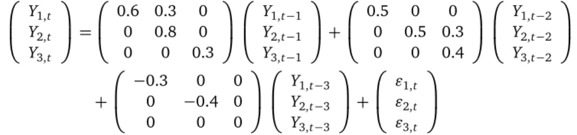
To show the strong efficiency of our model selection method we have generated a three-variable time series Yt = (Y1,t,Y2,t,Y3,t)0 of 300 observations from the following stationary
VAR process
Y1,t
Y2,t
Y3,t
=
0.6 0.3 0
0 0.8 0
0 0 0.3
Y1,t−1 Y2,t−1 Y3,t−1
+
0.5 0 0
0 0.5 0.3
0 0 0.4
Y1,t−2 Y2,t−2 Y3,t−2
+
−0.3 0 0
0 −0.4 0
0 0 0
Y1,t−3 Y2,t−3 Y3,t−3
+
"1,t
"2,t
"3,t
where ("1,t,"2,t,"3,t)0 is a standard normal random vector. Now we pretend that this true model is unknown to us. Our purpose is to find a VAR model that has the smallest BIC value among all the candidate models. Then we can consider this model as an estimate of the true model.
The results of using Lütkepohl’s LR testing scheme, presented in Table 1, show that H0(4):Φ3 =0 is the first null hypothesis that is rejected. Thus, the estimated order from the test is ˆP=3, and the full model can be represented as the index matrix VF={1}3×9. Then there are 227=134, 217, 728 candidate models in total for selection.
Table 1: Results of Lütkepohl’s LR test in Example 1 (Noteχ2
9(0.95) =16.92)
i Ho(i) VAR order underH0(i) λLR
1 Φ6=0 5 9.10
2 Φ5=0 4 6.16
3 Φ4=0 3 4.73
4 Φ3=0 2 274.05
5 Φ2=0 1 414.33
we obtained a 10×8 contingency table. Pearson’s χ2 test gives a p-value greater than 0.5. Therefore the null hypothesis of the independence of row and column factors can not be rejected. This means there is no significant evidence of the association; in another words, the generated VMSC series has reached its equilibrium.
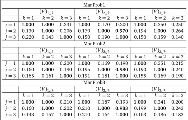
We continue and have totally generated 300×27 = 8100 models including the initial sample (not including the ignored 5×27 = 135 models). Denote the generated models as M1, . . . ,M8100 for convenience of presentation. We find there are 1189 different models amongM1 toM8100. We list in Table 2 the sample marginal probabilities of every component of V in between M1 and M2700, in between M1 and M5400 and in between M1 and M8100 respectively. We can see in any of the three classes the sample marginal probabilities corre-sponding to the non-zero components ofVo, which are
(V1,11,V1,12,V1,22,V1,33,V2,11,V2,22,V2,23,V2,33,V3,11,V3,22),
are all greater than 0.5 and even greater than 0.95, and those corresponding to the zero components of Vo are all less than 0.5. Moreover there is no obvious difference among the
marginal probabilities in the three classes. Therefore, based on the sample marginal probabil-ities of each component ofV, the true modelVois selected as the best model. The simulation study shows that it is sufficient to estimate 27×2×100=5400 models to identify the best model from the 227candidate models.
Table 2: Sample marginal probabilities of V in Example 1 among M1 to M2700 (Mar.Prob1), M1 to M5400
(Mar.Prob2) andM1to M8100(Mar.Prob3).
Mar.Prob1
(V)1,jk (V)2,jk (V)3,jk
k=1 k=2 k=3 k=1 k=2 k=3 k=1 k=2 k=3 j=1 1.000 1.000 0.231 1.000 0.170 0.200 1.000 0.350 0.250 j=2 0.130 1.000 0.206 0.170 1.000 0.970 0.194 1.000 0.264 j=3 0.220 0.143 1.000 0.150 0.190 1.000 0.150 0.159 0.140
Mar.Prob2
(V)1,jk (V)2,jk (V)3,jk
k=1 k=2 k=3 k=1 k=2 k=3 k=1 k=2 k=3 j=1 1.000 1.000 0.200 1.000 0.169 0.190 1.000 0.351 0.215 j=2 0.160 1.000 0.190 0.195 1.000 0.980 0.190 1.000 0.240 j=3 0.165 0.161 1.000 0.191 0.181 1.000 0.155 0.169 0.190
Mar.Prob3
(V)1,jk (V)2,jk (V)3,jk
k=1 k=2 k=3 k=1 k=2 k=3 k=1 k=2 k=3 j=1 1.000 1.000 0.210 1.000 0.187 0.193 1.000 0.341 0.200 j=2 0.160 1.000 0.202 0.210 1.000 0.983 0.199 1.000 0.243 j=3 0.143 0.157 1.000 0.210 0.164 1.000 0.163 0.186 0.183
227 candidate models to confirm our method’s effectiveness, but the result that the selected model is exactly the same as the true model simulating the observed series demonstrates the effectiveness and efficiency of this method.
Finally, the MLE of the best model Vois estimated to be
Y1,t Y2,t
Y3,t
=
0.66 0.26 0
0 0.80 0
0 0 0.29
Y1,t−1 Y2,t−1 Y3,t−1
+
0.50 0 0
0 0.55 0.24
0 0 0.38
Y1,t−2 Y2,t−2 Y3,t−2
+
−0.34 0 0
0 −0.45 0
0 0 0
Y1,t−3 Y2,t−3 Y3,t−3
with the standard errors for the corresponding coefficients of V1,11,V1,12,V1,22,V1,33,V2,11, V2,22,V2,23,V2,33,V3,11,V3,22 being 0.051, 0.027, 0.049, 0.053, 0.058, 0.060, 0.050, 0.055, 0.048 and 0.049.
Example 2: Chinese Money Supply
In this example, we illustrate the application of the Gibbs sampler model selection method on the real data. We establish a VAR model using two time series between the first quarter of 1993 and the first quarter of 2007. The two series are the growth rate of China’s quarterly nominal M2 money supply and China’s quarterly Consumer Price Index (CPI). The data of nominal M2 supply and CPI are published on the website of the National Bureau of Statistics of China†.
M2 money supply is a measure of the amount of money in the economy, and is constructed as the sum of currency, current deposit accounts, savings and other term deposits. The amount of M2 money supply is controlled by a country’s central bank as the monetary policy. CPI, which can also be called the inflation rate, is the increase rate of price of goods purchased by average households. From a macroeconomic perspective, a major reason that the money supply is important is that, in the long run, the amount of money circulating in an economy and the general level of prices are closely linked. To explain this relationship, let us have a look at the famous “quantity equation”.
MV=PY
where M is money supply, V is a measure of the speed at which money circulates, P is the price level and Y is the real output. V is determined by current payments technologies and thus is approximately constant. Likewise, one can assume that the real output Y is approximately constant. If we use a bar over a variable to indicate that the variable is constant, we can rewrite the quantity equation as
M¯V=P¯Y
Then we see that the quantity equation can hold only if M and P rise at the same growth rate.
However, there are two explanations of the relationship between the two variables (see Bernanke, Olekalns and Frank[5, Chapter 8]). One is that a rapidly growing supply of money will lead to quickly rising prices, that is, inflation. Another explanation of the relationship is that some other reasons cause the inflation, then the central bank has to increase the money supply to accommodate to the increased money demand caused by the increased prices.
Both explanations agree that there is a close relationship between the growth rate of money supply and the growth rate of price (inflation rate). In fact, there is an extensive literature on VAR modelling of money supply and inflation. For example, Anderson, Hoffman and Rasche[3], Juselius and Toro [21], and Zhao, Chen and Gao[34]studied the relation between money supply and other economic variables including CPI of U.S., Spain and China respectively using VAR models. However, all the established VAR models are unrestricted ones. The subset VAR model has not been found in use.
To investigate the relationship between the two variables in more detail we establish a subset VAR modelling frame. First of all, for a specification of VAR model it requires to examine the stationarity of the observed time series for the variables. We choose to use the Phillips-Perron unit root test [26] to examine this. Listed in Table 3 are the results for the growth rate of China’s M2 (denoted as M2r), the first order difference of the growth rate of the M2 (denoted as DM2r), CPI and the first order difference of the CPI (denoted as DCPI). From the table we see that the test rejects the null hypothesis of a unit root in DM2r and DCPI, but fails to reject the null hypothesis of a unit root in M2r and CPI at any of the reported significance levels. The tests strongly support that both growth rates of M2 and CPI are I(1). Thus, we are to establish a VAR model using the first order differences of both DM2r and DCPI.
Table 3: Results of Phillips-Perron unit root test in Example 2
test statistic 1% critical value 5% critical value
M2r -2.74 -3.55 -2.91
DM2r -5.81 -3.55 -2.91
CPI -1.57 -3.55 -2.91
DCPI -3.63 -3.55 -2.91
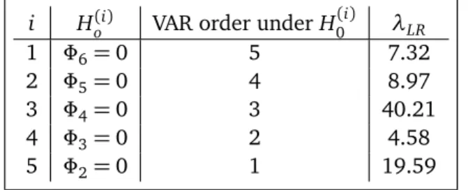
Table 4: Results of Lütkepohl’s LR test in Example 2 (Noteχ2
4(0.95) =9.49)
i Ho(i) VAR order underH0(i) λLR
1 Φ6=0 5 7.32
2 Φ5=0 4 8.97
3 Φ4=0 3 40.21
4 Φ3=0 2 4.58
5 Φ2=0 1 19.59
Having done the above preparation, we perform the model selection with λ= 0.8, and with AIC being used as the selection criterion. We generate 105 segments in each run. Then we use the method of Qian and Field[28]to test the equilibrium of the generated AIC values. To reduce the initialization effect of the Gibbs sampler we omit the first 5 segments in each sequence. Further, rather than take the last model of each segment to form a sample of size 100, we use all the 1800 models as the sample in each sequence. Ap-value being greater than 0.5 is obtained, suggesting we have reached the equilibrium.
Applying the model selection methods proposed, we have obtained the results listed in Ta-ble 5, which are the sample marginal probabilities of the components ofV from the 1800 mod-els generated. The sample marginal probabilities of (V0,1,V1,22,V2,21,V2,22,V4,11, V4,21,V4,22) are seen to be all greater than 0.5. We can thus identify the best model as
1 0 0 0 0 0 0 1 0 0 0 1 1 1 0 0 1 1
,
and have an AIC value 307.4237. After estimating the coefficients using the MLE the estimated VAR model is
DM2r=−0.505−0.522×DM2r(−4)
DCPI=0.377×DCPI(−1)−0.169×DM2r(−2) +0.476×DCPI(−2) +0.197×DM2r(−4)−0.507×DCPI(−4)
where DM2r(−4)is the lag 4 observation of DM2r and the other terms are similarly defined.
Table 5: Sample marginal probabilities ofV in Example 2 among M1 to M1800
(V)0,j (V)1,jk (V)2,jk (V)3,jk (V)4,jk
k=1 k=2 k=1 k=2 k=1 k=2 k=1 k=2 j=1 0.590 0.250 0.259 0.280 0.228 0.440 0.100 1.000 0.326 j=2 0.315 0.270 1.000 0.980 1.000 0.230 0.378 1.000 1.000
6. Conclusion
In this paper we propose a Gibbs sampler algorithm for subset VAR model selection involv-ing a large number of candidate models. This computinvolv-ing method is very useful in subset VAR model selection but has not been well studied before. The key feature of our proposed method is that we can generate a series of candidate models from an induced probability distribution in such a way that the best model will tend to appear among the earliest and the most frequent if the number of the models generated is large enough. We have developed several empirical solutions to tackle various complications that may be encountered in practice. It shows that the method is computationally feasible and effective in dealing with these difficulties.
ACKNOWLEDGEMENTS The project underlying this paper is supported by the International Cooperation and Exchange Program of National Natural Science Foundation of China (NSFC) (Grant No.71301070002).
References
[1] H. Akaike. Information theory and an extension of the maximum likelihood principle. In B.N. Petrov and F. Csáki, editors, Proceedings of Second International Symposium on Information Theory, pages 267–281, Budapest, 1973. Académiai Kiadó.
[2] H. Akaike. A Bayesian analysis of minimum AIC procedure. Annals of the Institute of Statistical Mathematics, 30(Part A):9–14, 1978.
[3] R. G. Anderson, D. L. Hoffman, and R. H. Rasche. A vector error-correction forecasting model of the US economy. Journal of Macroeconomics, 24:569–598, 2002.
[4] P. Bearse and H. Bozdogan. Subset selection in vector autoregressive models using the genetic algorithm with informational complexity as the fitness function.Systems Analysis Modelling Simulation, 31:61–91, 1998.
[5] B. S. Bernanke, N. Olekalns, and R. H. Frank.Principles of Macroeconomics.McGraw-Hill Australia, North Ryde, NSW, 2005.
[6] S. P. Brooks, N. Friel, and R. King. Classical model selection via simulated anneal-ing.Journal of the Royal Statistical Society Series B Statistical Methodology, 65:503–520, 2003.
[7] G. Casella and E.I. George. Explaining the Gibbs sampler. The American Statistician, 46(3):167–174, 1992.
[9] J. Cui, D. Pitt, and G. Qian. Model selection and claim frequency for workers’ compen-sation insurance. Astin Bulletin – The Journal of the International Actuarial Association, 40(2):779–796, 2010.
[10] W. Enders.Applied Econometric Time Series. Wiley, New York, 1995.
[11] W. Enders.Applied Econometric Time Series, 2nd edition. Wiley, New York, 2004.
[12] R. F. Engle and C. W. J. Granger. Cointegration and error correction: Representation, estimation and testing.Econometrica, 50:987–1007, 1987.
[13] E. I. George and R.E. McCulloch. Approaches for bayesian variable selection. Statistica Sinica, 7:339–373, 1997.
[14] C. W. J. Granger. Some properties of time series data and their use in econometric model specification. Journal of Econometrics, 16:121–130, 1981.
[15] C. W. J. Granger, M.L. King, and H. White. Comments on the testing economic theories and the use of model selection criteria. Journal of Econometrics, 67:173–187, 1995. [16] J. D. Hamilton. Time Series Analysis. Princeton University Press, New Jersey, 1994. [17] E. J. Hannan. The estimation of the order of an ARMA process. Annals of Statistics,
8:1971–1081, 1980.
[18] E. J. Hannan and B. G. Quinn. The determination of the order of an autoregression process. Journal of the Royal Statistical Society Series B Statistical Methodology, 41:190– 195, 1979.
[19] J. A. Howe and H. Bozdogan. Predictive subset VAR modeling using the genetic algo-rithm and information complexity. European Journal of Pure and Applied Mathematics, 3(3):382–405, 2010.
[20] C. M. Hurvich and C. L. Tsai. Regression and time series model selection in small sam-ples. Biometrika, 76:297–307, 1989.
[21] K. Juselius and J. Toro. Moneteray transmission mechanisms in spain: The effect of monetization, financial deregulation, and the EMS. Journal of International Money and Finance, 24:509–531, 2005.
[22] T. R. Liu, M. E. Gerlow, and S. H. Irwin. The performance of alternative VAR models in forecasting exchange rates. International Journal of Forecasting, 10:419–433, 1994. [23] H. Lütkepohl. New Introduction to Multiple Time Series Analysis. Springer-Verlag,
Hei-delberg, 2005.
[25] J.H.W. Penm and R. D. Terrell. On the recursive fitting of subset autoregressions.Journal of Time Series Analysis, 3:43–59, 1982.
[26] P. Phillips and P. Perron. Testing for a unit root in time series regression. Biometrika, 75:335–346, 1988.
[27] G. Qian. Computations and analysis in robust regression model selection using stochas-tic complexity. Computational Statistics, 14:293–314, 1999.
[28] G. Qian and C. Field. Using MCMC for logistic regression model selection involving large number of candidate models. In K.T. Fang, F.J. Hickernell, and H. Niederreiter, editors, Selected Proceedings of the 4th International Conference on Monte Carlo & Quasi-Monte Carlo Methods in Scientific Computing, pages 460–474, Hong Kong, 2002. Springer. [29] G. Qian and X. Zhao. On time series model selection involving many candidate ARMA
models. Computational Statistics & Data Analysis, 51:6180–6154, 2007.
[30] C. P. Robert (ed.).Discretization and MCMC Convergence Assessment.Springer, New York, 1998.
[31] G. Schwarz. Estimating the dimension of a model.Annals of Statistics, 6:461–464, 1978. [32] C. A. Sims. Macroeconomics and reality. Econometrica, 48:1–48, 1980.
[33] A. Zellner. An efficient method of estimating seemingly unrelated regressions and tests of aggregation bias. Journal of the American Statistical Association, 57:348–368, 1962. [34] X. Zhao, F. Chen, and T. Gao. Research on the transmission mechanism of China’s