Data Fusion Using Weighted Likelihood

Vol. 5, No. 3, 2012, 333-356

ISSN 1307-5543 – www.ejpam.com

Data Fusion Using Weighted Likelihood

Pengfei Guo, Xiaogang Wang, Yuehua Wu

Department of Mathematics and Statistics, York University, Toronto, Canada

Abstract. This article proposes to perform data fusion by using an adaptive weighted likelihood func-tion when data sets are available from related populafunc-tions. The main objective of data fusion is to integrate information from different sources to improve the quality of inference when the sample size from the target population is small or moderate. The weighted likelihood function is employed simply as an instrument to facilitate the data fusion process. The weighted likelihood method has information-theoretic justification and embraces the widely used classical likelihood method which utilizes only on the data set from the target population. The degree of information integration in the proposed data fusion process is determined by the likelihood weights which should be chosen in a reasonable and adaptive way. The major challenge in the proposed data fusion process is then to choose likelihood weights adaptively and effectively when the deterministic relationships among all related parameters are unknown. We propose adaptive likelihood weights based on the estimated likelihood ratio. We show that the data fusion involving all relevant data sets could significantly improve the mean squared error (MSE) of the classical maximum likelihood estimator which only uses data set from the target population. It also increases the power for hypothesis testing. The proposed estimator is shown to be consistent and asymptotically normally distributed in the framework of generalized linear models. The advantage of the proposed weighted likelihood estimator for linear models is illustrated numerically by a simulation study. A real data example is also provided.

2010 Mathematics Subject Classifications: 62F12, 62J05, 62J12

Key Words and Phrases: Cross-validation, Nonparametric regression, Relative likelihood ratio, Semi-parametric estimation, Weighted likelihood

1. Introduction

In clinical trials for medical research, a common problem that often arises is how to ef-ficiently estimate the parameter of interest when the sample size from the population of in-ferential interest is small due to the cost or other limitations associated with the experiment. When the sample size from the population of inferential interest is small and observations from related studies are available, one important question is whether there is any merit to

∗_{Corresponding author.}

Email addresses:pguomathstat.yorku.a(P. Guo),stevenwmathstat.yorku.a(S. Wang), wuyhmathstat.yorku.a(Y. Wu)

combine information from populations that are known to be different than the population of inferential interest.

The classical likelihood method would concentrate solely on the sample from the the target population without incorporating other relevant information. The advantage of doing so is to avoid possible bias or contamination of the data sampled directly from the target population. The maximum likelihood estimator (MLE) is well known to enjoy asymptotic properties such as consistency and asymptotic normality. It is one of the most widely used method in statistical inference. However, the asymptotic properties are of little help when the sample size is small or very moderate. The MLE could provide quite misleading results due to a insufficient sample size. By contrast, the Bayesian method can effectively combine information when the parameters from these populations are assumed to be random variables from a hyper-distribution. It has many advantages since prior information can be formally incorporated and the inferences are conditional on all the data. Bayesian inference might be computationally intensive for non- trivial cases. It is well known, however, the powerful Monte Carlo Markov Chain method could be computationally intensive and challenging for the high dimensional case when a conjugate prior can not be assumed.

For exploratory purposes, we propose to integrate all available information through a data fusion process based on an adaptive weighted likelihood function. The weighted likeli-hood function that we employ can be very adaptive and easy to implement. Since there are many weighted likelihoods proposed for various purposes, it is necessary to provide an brief overview and avoid any possible confusion later on. [4]introduced the idea of local likeli-hood to derive local inference. [2] defined her version of local likelihood in the context of non-parametric regression. [17]presented the general form of the local likelihood. [9]and

[10] proposed their relevant weighted likelihood function to combine information in which the weights are very general. [12]proposed their adaptive weights when the time trend is present. [11]reviewed most related weighted likelihood methods proposed in the literature. All the aforementioned weighted likelihood methods focus on a setting in which the number of populations goes to infinity. In this article, however,we focus on situations in which the number of populations is actually fixed. For example, one might be interested in the efficacy of one particular treatment when the results of the current and several historical clinical trials are available.

Extending the relevant weighted likelihoodby[9], [21]proposed their version of the WL when the number of populations is fixed. We now briefly their weighted likelihood function as follows. Suppose that we observe independent random response vectors Y₁, . . . ,Y_m with probability density functions f(.;θ1), . . . ,f(.;θm), whereYi = (Yi1, . . . ,Yini)

T_{,i=1, 2,· · ·,m.} Further suppose that only population 1, in particularθ1, an unknown vector of parameters, is

of inferential interest. Given data,Y₁=y₁, the classical likelihood would be

L₁(y₁,θ1) =

n1 Y

j=1

f(y_1j;θ1).

y= (y₁,y₂,· · ·,y_m), the weighted likelihood (WL) forθ1 is defined as

WL(y;θ1) =

m

Y

i=1

ni Y

j=1

f(yi j;θ1)λi,

where λ = (λ1, . . . ,λm), the “weights vector”, must be specified. We emphasize that the

parameters from the related populations, θ2, . . . ,θm, which are unknown, do not appear in

the WL, since the inferential interest focuses onθ1 of the first population.

The WL estimator (WLE) for θ1, say ˜θ1, is defined as the maximizer of the objective

function WL(y;θ1):

˜

θ1=arg sup

θ1∈Θ

WL(y;θ1).

In order for the weighted likelihood to be effective, the weights must be chosen adaptively so that all information obtained from related population must be evaluated to determine their relevance. [7]proposed a cross-validatory procedure for weights selection and showed that the resulting WLE is consistent and asymptotically normal. However, the cross-validatory approach is challenged with the following problems: (a) it is computationally intensive if the WLE does not have an analytical form, and (b) numerical performances could be unstable when the sample sizes are unequal or the sample sizes are very small. Thus, we propose a simple and effective method to choose the likelihood weights adaptively. This method is better than the cross-validated weights proposed by[7]in that its computation is robust and implementation is straightforward. More importantly, it avoids all the numerical problems with the cross-validated weights when the sample sizes are small or unequal. We derive the consistency and asymptotic distribution of the resulting WLE.

The article is organized as follows. In Section 2, we develop a WL procedure. The asymp-totic properties of the WLE for generalized linear models using the proposed adaptive weights are presented in Section 3. Section 4 presents the results from simulation experiments that illustrate the numerical performance of our method. Section 5 shows how to obtain the em-pirical distribution of the WLE by bootstrap. Section 6 analyzes a real data set from by using the proposed approach. Section 7 provides conclusions and discussions.

2. The Weighted Likelihood and Adaptive Weights

2.1. The Weighted Likelihood

We assume the existence of the m population density functions are unknown and play purely conceptual roles. More specifically, assumeσ-finite probability spaces

(Ω,F,µi),i=1, 2, . . . ,m, with probability measures µi’s that areabsolutely continuous with

respect to one another. The existence of a σ-finite measure ν that dominates theµi’s then

follows. We take the fi to be the Radon-Nikodym derivatives of µi with respect to ν for

i=1, 2, . . . ,m.

Suppose that we observe independent random response vectorsY₁, . . . ,Y_mwith probabil-ity densprobabil-ity functions f(.;θ1), . . . ,f(.;θm), where Yi= (Yi1, . . . ,Yini)

suppose that only population 1, in particular θ1, an unknown vector of parameters, is of

inferential interest. Given data,Y₁=y₁, the classical likelihood ofθ1is defined by

L1(y1;θ1) =

n1 Y

j=1

f(y1j;θ1).

Similarly, we can define the likelihood for eachθi as follows:

L_i(y_i,θ1) =

ni Y

j=1

f(y_{i j};θi).

wherei=2,_{· · ·},m.

If all parameters are not related in any way, the correct likelihood for θ1 should be

L₁(y₁;θ1). However, L1(y1;θ1)would not be the correct likelihood if there exist functional

relationship among all parameters. To be more specific, assume that

θ2 = g1(θ1), . . . ,θm = gm(θ1), where gi are measurable functions of θ1. Furthermore, if all

observations from different populations are independent of each other, the likelihood of θ1

involving all samples should be

˜_{L(y1,· · ·,ym;θ1) = L1(y1,θi) ×}

m

Y

i=2

L_i(y_i,g_i(θ1)).

We observe that all parameters,θ2, . . . ,θm disappeared from the above likelihood since they

are replaced by g2(θ1), . . . ,gm(θm)respectively. We see that all data sets are integrated into

one likelihood function that we call fusion likelihood.

When the functional relationship, g_i, are indeed known, we can derive the estimating equation by consider the following:

log ˜L(y₁, . . . ,y_m;θ1)

∂ θ1

= logL1(y1;θ1)

∂ θ1

+

m

X

i=2

logL_i(y_i;θ_i)

∂ θi

g_i(θ1)

∂ θ1

= logL1(y1;θ1)

∂ θ1

+

m

X

i=2

w_i(θ1)

logL_i(y_i;θi)

∂ θi

.

where w_i(θ1) = ∂gi(θ1)/∂ θ1,i = 2,· · ·,m. By setting the above function to be zero, we

obtain an estimating equation forθ1 which is based on all available data.

In practice, however, the functional form of g_i’s are not known. Therefore, the analytical forms of g_i’s are simply not available. When facing such a difficulty, one could abandon the data fusion process and proceed with L1 by severing the connections among all parameters.

The alternative is try to incorporate information from other sources in a meaningful way. This must be done in a reasonable and careful fashion without the knowledge of the link func-tions g_i,i=2,_{· · ·},m. First, we must adopt a meaningful measure to evaluate the discrepancy among the probability density distributions when the parameters are known. Second, we must tackle the problem without the knowledge of the true values of the parameters. To re-solve the first challenge, we propose to use some general measure for information discrepancy to characterize the connections among all parameters. Entropy or relative entropy has been widely used in information theory. For density functions, g₁(x)and g₂(x), with respect to a

σ₋finite measure ν, the relative entropy, also calledKullback-Leiblerdivergence, is defined as:

K L(g₁,g2) =E1

logg1(X) g₂(X)

=

Z

log g1(x)

g₂(x)g1(x)dν(x). (1) In this expression, log(g₁(x)/g2(x))is defined as+∞, ifg1(x)>0 andg2(x) =0. Therefore

the expectation could be+∞. Although log(g₁(x)/g₂(x))is defined as−∞when g₁(x) =0 and g₂(x) > 0, the integrand, log(g₁(x)/g₂(x))g₁(x) is defined as zero in this case. It is widely used in information theory. Detailed discussions and application of the entropy in information theory can be found in [19]. Some theoretical properties of the entropy can be found in [14]. In particular, the relative entropy is not symmetric and therefore not a distance. The relative entropy, also known as Kullback-Leibler divergence, is also called the entropy loss. [20] introduce it as a performance criterion in estimating the multinormal variance-covariance matrix. [15] shows the entropy is a loss function in a Bayesian frame-work. [18] provides detailed discussions on the relative entropy including the connection between Fisher information and relative entropy.[13]has shown that the classical maximum likelihood principle can be considered a method of asymptotic realization of an optimum estimate with respect to the relative entropy.

Since the metric of the manifold that connects all the parameters can not be specified, we now define the neighborhood enveloping by [17]. For any fixed value ofθ1, the parameter

of the population of inferential interest, we can define a neighborhood by using the relative entropy as

N_f1(ε) =∪_θ∈Θ{f(θ):I(f(θ),f₁)≤ε}, (2) where f₁= f(x,θ1)andε≥0.

Assume that the density functions, f1, . . . ,fm∈V, are all assumed to be continuous where

V is a reflexive Banach space. Although V can be quite arbitrary, we take V = Lp=Lp(Ω,ν). It is known that the Lp spaces (1 < p < ∞) are reflexive but that L1 is not [see 16, for example]. Fori=2, . . . ,m, we define

Ei={g∈Lp:||g−fi||p<Ci,

Z

f_i(x)log g(x)

f_i(x)dν(x)≤ai, Z

g(x)dν(x) =1,g(x)>0}, (3)

where ai ≥0 and Ci, i=2, 3, . . . ,m, are constants. We then define the interception of these

individual enveloping neighborhood.

We remark that the setE will be bounded with respect to the Lp norm and non-empty if the constraints are not too restrictive. The latter is assumed throughout.

Thus, for a given set of density functions, f₁(x) being primary, we seek a probability density function g∈ E which minimizesI(f1,g) =

R

f1(x)log g

(x)

f1(x)dν(x)over all probability densities, g, satisfying

I(f_i,g)≤a_i, i=2, . . . ,m, (5) wherea_i,i=2, 3, . . . ,m, are non-negative constants.

[6]showed that the the optimal solution takes the form of amixing distribution:

g∗=

m

X

i=1

λi fi(x), (6)

where g∗is the optimal solution for optimization probelm described above.

Assuming that f_i are members of one parametric family while the difference is due to different value for the parameter, i.e. f_i(x) = f(x;θ_i). Without the knowledge of the exact values forθi,[6]show that the weighted likelihood function:

WL(y;θ1) =

m

Y

i=1

ni Y

j=1

f(yi j;θ1)λi, (7)

is the correct device to used by following the argument of[13]. The weights are functions of theλi’s which measures the discrepancies among all parameters.

We remark that this classical likelihood is embraced by the proposed likelihood by setting the weights to be zero for relevant samples. In addition,[5]showed that the estimator derived from the weighted likelihood function can be viewed as an approximate Bayes decision by following the same argument by[3]. The coefficients a_i’s, however, are not known since the exact functional form of the connections among all parameters are not assumed to be known. Therefore, the weights must be chosen adaptively to avoid introduction of significant bias into the inference for the target population.

2.2. Adaptive Weights Based on Likelihood Ratio

Since the weighted likelihood is the chosen instrument for the data fusion process, the likelihood weights play a central role in integrating all relevant information in a meaningful way. As we have seen in previous section, the likelihood weights should be chosen to reflect the true relevance between a relevant sample and the target population. Without any prior knowledge, the evidence expressed in the relevant sample should be the only source for eval-uation and determination of a set of appropriate weights. The fundamental question is how to measure the discrepancy between to two populations that could be related.

In a likelihood ratio context, a likelihood-ratio test is a statistical test for making a decision between two hypotheses based on the value of this ratio.

to the hypothesis test, it implies that the two parameter values are too different in the context of likelihood ratio. Following the same line of argument, we propose to use the likelihood ratio as a measure of discrepancy. Since the true values of the parameters are not known, it is natural to use estimated likelihood ratio with the parameter values replaced by corresponding MLE estimates.

Given a parametric density function f₁ and a sampleY₁= (Y₁₁,Y₁₂, . . . ,Y_1n

1), the classical likelihood ratio for testing a null hypothesis is based on the following

LR= sup_Ω

H

n1 Q

j=1

f₁(Y_1j;θ1)

sup_Ω

n1 Q

j=1

f₁(Y_1j;θ1)

,

whereΩ_H is a subspace in the parameter space under the null hypothesisH.

Assume that the likelihood function attains an unique maximum inΩ_H andΩrespectively. Denote the maximizers as θb₁H and θb1 respectively. The likelihood ratio (LR) can then be

rewritten as

LR=

n1 Q

j=1

f₁(Y_1j;θb₁H)

n1 Q

j=1

f₁(Y_1j;θb1)

.

Therefore, the validity of the proposed hypothesis is evaluated according to the likelihood ratio.

By using a similar idea, we propose to choose likelihood weights by using the estimated pairwise likelihood ratio. For simplicity, let m=2, i.e., there is only one related population together with the target population. Let θb2 denote the estimate derived from the second

sample. We consider the estimated pairwise likelihood ratio (PLR) as follows:

γi=P LRi =

n1 Q

j=1

f1(Y1j;θbi) n1

Q

j=1

f1(Y1j;θb1)

, i=1, 2.

It then follows thatγ1equals to 1. Furthermore, we haveγi≤1,i=2, . . . ,mby the definition

of the MLE.

The likelihood weightsλ1andλ2will then be chosen as

λ1=

1

1+γ₂, λ2= γ2

1+γ₂.

For the simple linear models presented before, a simplification yields that the WLE ofβ1takes

the following form:

b

βWLE

where

w1=

n1 P

j=1

x2_1j

n1 P

j=1

x₁2_j+γ2

n2 P

k=1

x₂2_k

andw2=

γ2

n2 P

k=1

x2_2k

n1 P

j=1

x₁2_j+γ2

n2 P

k=1

x₂2_k .

To further illustrate the behavior of the proposed likelihood weights, we revisit the simple linear models given by Equation (1). It then follows that

γ2 = exp

  −

1 2σ2

1

n1 X

j=1

(y_1j−βbMLE

2 x1j)2+

1 2σ2

1

n1 X

j=1

(y_1j−βbMLE

1 x1j)2

   = exp   −(βb

MLE

1 −βb

MLE

2 ) 2

n1 X

j=1

x₁2_j/(2σ2₁)   .

Sinceλ2=1/(1+γ2), we then have

λ2=

1

1+exp (

(βbMLE

1 −βb

MLE

2 )2

n1 P

j=1

x2_1j/(2σ2₁) ).

Thus the proposed likelihood weight for the second sample is a function of the estimated dif-ference between the regression coefficients, the variance of the error terms and the “variance” of the covariate. For a fixed design matrix, a large difference betweenβbMLE

1 andβb

MLE

2 will

re-duce the assigned importance to the second sample. On the other hand, a large variance in the first model would result in a bigger value for the weight assigned to the second sample.

2.3. Estimation with Fixed Likelihood Weights

In this section we develop the WL procedure for the linear models as an illustration. For simplicity, we assume that m= 2 in Sections 2.1 and 2.2. Extension to the case of m> 2 is straightforward. Assume that data_{x1j,y1j;j=1, . . . ,n1}and{x2k,y2k;k=1, . . . ,n2}are

generated from the following models:

y_1j = β1x1j+εj, εj ∼N(0,σ21), j=1, . . . ,n1,

y2k = β2x2j+ek; ek∼N(0,σ22), k=1, . . . ,n2,

(8)

where the{x1j,j=1, . . . ,n1;x2j,k=1, . . . ,n2}are fixed. Assume that{εj}’s andek’s arei.i.d.

respectively. The error terms from these two models are assumed to be independent as well. For the purpose of our demonstration we assumeσ1 andσ2 are known although that would

rarely be the case in practice. Denotey₁= (y11,y12, . . . ,y1n1) T_{, and}

Suppose that the parameter, β1, is of primary inferential interest. The parameter β2 is

thought or expected to be not too different fromβ1 due to the “similarity” of the two

experi-ments. Note that a bivariate distribution is not assumed in the above model. Assuming marginal normality, the marginal likelihoods forβ1andβ2 are

L₁(y₁;β1)∝

n1 Y

j=1

exp ¨

−(y1j−β1x1j) 2

2σ2 1

« ,

and

L₂(y₂;β2)∝

n2 Y

k=1

exp ¨

−(y2k−β2x2k) 2

2σ2 2

« .

A direct calculation deduces the MLE ofβ1 andβ2as follows

b

βMLE

1 =

  

n1 X

j=1

x2_1j   

−1

n1 X

j=1

x_1jy_1j, andβbMLE

2 =

n2 X

k=1

x₂2_k !−1 _n

2 X

k=1

x_2ky_2k.

If one knows that β1 and β2 are similar to each other according to past studies or expert

opinions, then it is reasonable to expect that this information might be used to yield a better estimate of the parameterβ1.

The WL for inference aboutβ1can be represented as:

WL(β1;y1,y2) = L

λ1

1 (y1;β1)L

λ2

2 (y2;β1), (9)

where λ1 andλ2 are weights selected according to the relevance of the likelihood to which

they attached. The non-negative requirement for the weights is not assumed in the formu-lation although the optimum weights should be non-negative according to the assertion by

[6].

It is worth noting thatL₂(y₂;β₁)instead ofL₂(y₂;β₂)is used to define WL(β₁)sinceβ₁is of our primary inferential interest at this stage and the marginal distributions of the elements of the Y₂ are thought to resemble the marginal distributions of those of the Y₁. Note that the WL for θ1 depends on the distribution of the Y1. However, it does not depend on the

distribution ofY₂. Notice that the joint distribution of the Y₁ andY₂ does not appear in the formulation of the WL forθ1 and no assumptions are made about it.

The WLE of β1 is obtained by maximizing the weighted likelihood function for given

weightsλ1andλ2. It follows from (9) that

log{WL(β1)}=λ1log{L1(y1;β1)}+λ2log{L2(y2;β1)}.

Note that

∂log{WL(β1)}

∂ β1

= λ1 2σ₁2

n1 X

j=1

x1j(y1j−β1x1j) +

λ2

2σ2₁

n2 X

k=1

A simplification yields the WLE ofβ1as follows

b

βWLE

1 =w1βb1MLE+w2βb2MLE. (10)

where

w1=

λ1

n1 P

j=1

x₁2_j

λ1

n1 P

j=1

x2_1j+λ2

n2 P

k=1

x₂2_k

andw2=

λ2

n2 P

k=1

x2_2k

λ1

n1 P

j=1

x₁2_j+λ2

n2 P

k=1

x₂2_k .

It can be seen that the WLE of β1 is a linear combination of βb1MLE andβb

MLE

2 , under the

over-simplified model. The WLE ofβ1 coincides with the MLE ofβ1obtained from the first if the

weight for the second marginal likelihood function is set to be zero. Therefore, the weights w₁ andw₂reflect the importance ofβbMLE

1 andβb

MLE

2 .

Letβ₁0 andβ₂0 be the true values of the parametersβ1 andβ2 respectively. If one knows

that|β0

1−β20| ≤C, whereC is a known constant according to past studies or expert opinions,

we then have the following theorem.

Theorem 1. Under the normality assumption with known variances, the WLE β˜WLE

1 takes the

form

˜

βWLE

1 (w1,w2) =w1βb1MLE+w2βb2MLE,

where w₁+w₂ = 1, 0 < w₁ ≤ 1, 0 ≤ w₂ < 1. Furthermore, |β₁0−β₂0| ≤ C, C > 0, then

|E(β˜1−β10)| ≤w2 C. In addition,

max

w1,w2

M SE(β˜WLE

1 )<M SE(βb

MLE

1 )if and only if

M

M+1<w1<1, where

M=

C2+σ2 2

‚_n 2 P

k=1

x2_2k Œ₋1

−σ2 1

n1 P

j=1

x₁2_j !−1

2σ2 1

n1 P

j=1

x₁2_j

!₋1 .

In addition, Var(β˜WLE

1 )<Var(βb

MLE

1 )ifmaxw1,w2M SE(β˜ WLE

1 )<M SE(βb

MLE

1 ).

Thus, for small value of C, the WLE could have smaller MSE and variance simultaneously with the cost of small bias. The magnitude of the bias is controlled by the weight assigned to the second population. The lower bound for the weight w₁ is connected with the worst MSE of the WLE instead of the optimal one.

3. Asymptotic Properties

In this section we investigate the asymptotic properties of the WLE in the framework of generalized linear models (GLM) for simple presentation. The GLMs have the following structure. The sample Y = (Y₁, . . . ,Y_n) _{∈ ℜ}n _{has independent components and Y}

i has the

p.d.f.

exp

ηiyi−ζ(ηi)

φi

h(yi,φi), . . . ,n,

w.r.t. aσ-finite measureν, whereη_i andφ_i are unknown,φ_i>0,

ηi∈Ξ ={η: 0<

Z

h(y,φ)eηy/φdν(y)<_{∞} ⊂ ℜ}

for alli,ζandhare known functions, andζ′′(η)>0 is assumed for allη∈Ξ◦, the inferior of Ξ. Note that the p.d.f. belongs to an exponential family ifφis known. As a consequence, for i=1, . . . ,n,

E(Y_i) =ζ′(ηi)

△ =µ(ηi),

Var(Y_i) =φζ′′(ηi).

It is assumed thatηi is related toXi, theith value of ap-vector covariates, through

g(µ(ηi)) =βTXi, i=1, . . . ,n.

In GLM,β is the parameter of interest andφi’s are considered to be nuisance parameters.

The range of β is assumed to be B = {β :(g◦µ)−1(βTx)∈Ξ◦∀x ∈ X }, whereX is the range ofX_i’s. It is often assumed that

φi=φ/ti, i=1, . . . ,n,

with unknownφ >0 and known positivet_i’s.

Letθ = (β,φ)andψ= (g◦µ)−1, then the log-likelihood function is

logl(θ) =

n

X

i=1

–

logh(y_i,φ/t_i) + ψ(β

T_X

i)yi−ζ(ψ(βTXi))

φ/t_i

™

and the score function forβ is

sn(β) =

∂ logl(θ)

∂β =

1

φ

n

X

i=1

{[yi−µ(ψ(βTXi))]ψ′(βTXi))tiXi}.

Let

Mn(β) = n

X

i=1

Then the Fisher information evaluated atβ is

In(β) =Var

∂ logl(θ)

∂β

=Mn(β)/φ.

We now present the asymptotic properties for the relevant weighted likelihood estimator and the hypothesis testing based on this estimator. We use double index as the subscript of observations and establish the following notations.

• β0: The true parameter value of main group.

• y1j,j=1, . . . ,n1 are the observations from main group.

• y_2j,j=1, . . . ,n₂ are the observations from contamination group.

• wl(β) =P2_i=1Pni

j=1wi jlogf(yi j|xi,β) =

P2

i=1

Pni

j=1wi jli j(β).

• l(β) =P2_i=1Pni

j=1logf(yi j |xi,β) =

P2

i=1

Pni

j=1li j(β).

Besides the regularity conditions and assumptions given in [1], we need the following additional assumptions for the present problem.

(A1) The information matrix of main group I_n1(β0)is positive definite, and the eigenvalues

ofn−₁rI_n1(β₀)are bounded, for some r >0, so are the eigenvalues ofnr₁I_n−1

1 (β0). That is, there exist constantsc₁ andc₂, such that

c1≤λminnr1I− 1

n1 (β0)≤λmaxn

r

1I− 1

n1 (β0)≤c2.

(A2) There exists a neighborhood ofβ0,O, such that for allβ∈Oand y2j, j=1, . . . ,n2,

E (

sup β∈O,1≤j≤n2

log

f(y_2j,β) f(y_2j,β0)

)

≤K,

whereK is a constant.

(A3) The proportion of contamination converges to 0 in the order ofn−1/2, i.e.,εn=o(n−1/2).

(A4) The criteria to choose weights guarantees that the weights are consistent. Assume the first n1 observations are from main group and the rest are from contamination group.

Then asn→ ∞andε_n→0,

w = (w₁, . . . ,w_n)T →v= (v₁, . . . ,v_n) = (1, . . . , 1 | {z }

n1

, 0, . . . , 0 | {z }

n2 )T.

Furthermore, max_i|w_i−v_i|=o(n−1/2).

Theorem 2. Under the regularity conditions specified in[1]and assumptions (A1)–(A4), there is a sequence of estimators{βˆn}such that

P(s_n( ˆβn) =0)→1

andβˆn→β0in probability.

Proof. In order to present the proof clearly, we use double index as the subscript of obser-vations. Then we need to specify the following notations.

• β₀: The true parameter of main group.

• γ₀: The true parameter of second group.

• y1j,j=1, . . . ,n1 are the observations from main group. • y_2j,j=1, . . . ,n₂ are the observations from second group.

• wl(β) =P2_i=1Pni

j=1wi jlogf(yi j|xi,β) =

P2

i=1

Pni

j=1wi jli j(β).

• l(β) =P2_i=1Pni

j=1logf(yi j|xi,β) =

P2

i=1

Pni

j=1li j(β).

Since there are two populations, we distinguish the score functions, Fisher information, design matrices in the following way. For main group, we denote them ass_n1(β),I_n1(β)andX; and for contamination group, we havesn2(β), In2(β)andZ. For simplicity, We useMn1 to denote M_n1(β₀).

Define the neighborhood ofβ₀,N_n

1(δ), δ >0, as

N_n1(δ) =_{β: kI_n1(β₀)1/2(β−β₀)_{k ≤}δ)_},

where In1(β0) is the Fisher information of the main group data evaluated at true valueβ0. Let ∂N_n1(δ) be the boundary of N_n1(δ). To proveβ →p β₀, it is sufficient to show for any

η >0, there existδ >0 andN>0, such that forn≥N and allβ ∈∂N_n

1(δ), we have

P(wl(β)−wl(β₀)<0 for allβ ∈∂N_n1(δ))>1−η. We start the proof by partitioningwl(β)−wl(β₀).

wl(β)₋wl(β₀)

=

n1 X

j=1

”

l_1j(β)−l_1j(β₀)—−

n1 X

j=1

(1−w_1j)”l_1j(β)−l_1j(β₀)—+

n2 X

j=1

w_2j”l_2j(β)−l_2j(β₀)—

△

=A−B+C.

Then we need to show thatBandC are dominated byA, which will follows fromBandC are o_p(1)since it is shown thatAisO_p(1)in[1].

In the following, we show that Bis dominated byA. Defines1_n−w 1 (β)as

s1_n−w

1 (β) =

∂

∂β

n1 X

j=1

(1−w_1j)l_1j(β)

= ‚

∂ logf(y₁₁,β)

∂β , . . . ,

∂logf(y_1n 1,β)

∂β

Œ   

1−w₁₁ .. . 1₋w_1n

1    

△

= €U₁, . . . ,U_n1ŠW₁

△

= S₁W₁.

Lets_n

1(β)be the score function for the main group, which can be similarly written as s_n1(β) =S₁1_n1,

where 1_n denotes the length-n vector with all element equal to 1. Then by taking Taylor expansion ofB, we have

B= (β−β₀)Ts1_n−w 1 (β0) +

1

2(β−β0)

T_∇s1−w n1 (γ

∗_)(β−β

0),

whereγ∗∈Nn1(δ). In the following, we will show that both these two terms areop(1). To show(β−β₀)T_s1−w

n1 (β0) =op(1), we need to show for anyǫ >0, lim

n→∞P(k(β−β0)

T_s1−w

n1 (β0)k< ǫ) =1 By Markov inequality, we have

P(k(β−β₀)Ts1_n−w

1 (β0)k< ǫ)≥1−( 1

ǫ)

2_Ek(β−β

0)Ts1n−1w(β0)k

2

and so it is sufficient to showEk(β−β₀)T_s1−w n1 (β0)k

2_→0.

Letλ=In1(β0)

1/2_(β−β

0)/δ, thenkλk=1 and

Ek(β−β₀)Ts1_n−w 1 (β0)k

2_=Ek(β−β

0)TS1W1k2

=EkδλTI_n−1/2

1 (β0)S1W1k

2_≤δ2_kW1k2_EkI−1/2

n1 (β0)S1k

2

=δ2kW1k2E n

t r[S₁TI_n−1

1 (β0)S1] o

=δ2kW1k2E

  

n1 X

j=1 UT_j I_n−1

Because the eigenvalues of I_n1(β₀)/nr₁ are bounded by assumption (A4), so are eigenvalues ofn₁rI−_n1

1(β0). That is

c1≤λmin(nr1I− 1

n1 (β0))≤λmax(n

r

1I− 1

n1 (β0))≤c2,

where c₁ andc₂ are constants. BecauseEUT_jU_k =0, let I_p be the p×p identity matrix, we have

Ek(β−β₀)Ts1_n−w 1 (β0)k

2_≤δ2_kW1k2 1

n1 E    n1 X

j=1

UT_j(n₁rI−_n1

1 (β0))Uj   

≤δ2_kW1k2 1

n₁E   

n1 X

j=1

UT_j[c₂Ip]Uj

  

≤δ2kW1k2 c2

n₁rc1

Ens_n1(β₀)T[n₁rI_n−1

1(β0)]sn1(β0) o

≤δ2kW1k2 c2

n₁rc1

E t rns_n1(β₀)T[nr₁I_n−1

1 (β0)]sn1(β0) o

=δ2kW1k2c2p

c1

.

Because maxi(1−wi) =o(n−1/2),kW1k2=o(1). Thenδ2kW1k2

c2p

c1 =o(1). So Ek(β−β₀)Ts1_n−w

1 (β0)k

2_{→0. This proves that the first term is o}

p(1).

In order to show the second term isop(1), we need to showk(β−β0)T∇s1n−1w(γ

∗_)(β−β

0)k

iso_p(1). Since

(β−β₀)T_∇s1_n−w

1 (γ)(β−β0) =δ

2_λT_I−1/2

n1 (β0)∇s

1−w n1 (γ)I

−1/2

n1 (β0)λ, it is sufficient to show

max

γ∈Nn₁(δ)

kI_n−1/2

1 (β0)∇s

1−w n1 (γ)I

−1/2

n1 (β0)k →0. Let

Rw_n

1(β) =

n1 X

j=1

(1₋w1j)[y1j−µ(ψ(βTXj))]ψ′′(βTXj)tjXjXTj ,

M_nw

1(β) =

n1 X

j=1

(1₋w1j)[ψ′(βTXj)]2ζ′′(ψ(βTXj))tiXjXTj .

Then

∇s1_n−w

1 (γ) = [R

w

n1(γ)−M

w

n1(γ)]/φ. So it suffices to show

max

γ∈Nn1(δ)

kM_n−1/2

1 M

w n1(γ)M

−1/2

and

max

γ∈Nn1(δ)

kM_n−1/2

1 R

w n1(γ)M

−1/2

n1 k →0. Because

kM_n−1/2

1 M

w n1(γ)M

−1/2

n1 k ≤max_j (1−w1j)kM −1/2

n1 Mn1(γ)M −1/2

n1 k. Using similar argument as in[1],_kM_n−1/2

1 Mn1(γ)M −1/2

n1 kis bounded by max

γ∈Nn1(δ)

kM_n−1/2

1 Mn1(γ)M −1/2

n1 k ≤

p_{p max}

γ∈Nn1(δ),j≤n1

|ϕ(γTX_j)/ϕ(βTX_j)|,

which converges to 0 sinceϕ is continuous and, forγ∈N_n

1(δ),|γ

T_X

j−βTXj|2→0. Because

maxj(1−w1j)→0, we have

max

γ∈Nn1(δ)

kM_n−1/2

1 M

w n1(γ)M

−1/2

n1 k →0.

Let

e_j = y_1j−µ(ψ(βTX_j)),

U_nw

1(γ) =

n1 X

j=1

(1₋w1j)[µ(ψ(βTXj))−µ(ψ(γTXj))]ψ′′(βTXj)tjXjXTj ,

V_nw 1(γ) =

n1 X

j=1

(1−w_1j)e_j[ψ′′(γTX_j)−ψ′′(βTX_j)]t_iX_jXT_j ,

W_nw

1(β) =

n1 X

j=1

(1−w_1j)e_jψ′′(βTX_j)]t_iX_jXT_j .

ThenRw_n

1(γ) = U

w

n1(γ) +V

w

n1(γ) +W

w

n1(β). Using a similar argument as above, we can show that

max

γ∈Nn₁(δ)

kM_n−1/2

1 U

w n1(γ)M

−1/2

n1 k →0. Note thatkM_n−1/2

1 U

w n1(γ)M

−1/2

n1 kis bounded by the product of

max

j (1−w1j)M

−1/2

n1

n1 X

j=1

|e_j|t_jX_jXT_j M_n−1/2

1 =op(1)

and

max

γ∈Nn₁(δ),j≤n1

|ψ′′(γTX_j)−ψ′′(βTX_j)|,

which can be shown to beo(1)using the same argument. Hence, max

γ∈Nn1(δ)

kM_n−1/2

1 V

w n1(γ)M

−1/2

Finally we need to show

max

γ∈Nn1(δ)

kM_n−1/2

1 W

w n1(β)M

−1/2

n1 k →0. SinceE(e_j) =0 ande_j’s are independent, it suffices to show that

n1 X

j=1

E|(1−w_1j)e_jψ′′(βTX_j)t_iXT_j M_n−1 1 Xj|

1+τ_→0

for someτ_∈(0, 1). It is trivial since max_j(1₋w1j)→0 and it is shown in[1]that n1

X

j=1

E|ejψ′′(βTXj)tiXTj M−

1

n1 Xj|

1+τ_→0.

Now we have shown that the first term and the remainder of the Taylor expansion of B are botho_p(1). SoB=o_p(1).

In the following we show thatC is dominated byA. By assumption (A5), we have

E|C| = E

n2 X

j=1

w2j

”

l2j(β)−l2j(β0)

—

≤

n2 X

j=1

w_2jE log

f(y_2j,β) f(y2j,β0)

≤ K

n2 X

j=1

w_2j

= K·n2o(n−1/2) → 0.

This impliesC →p0.

Theorem 3. Under the assumptions of Theorem 2, I1_n/2

1 (β0)( ˆβ−β0)→Np(0,Ip)

in distribution.

Proof. Let

sw_n(β) = ∂

∂β

2

X

i=1

ni X

j=1

wi jli j(β)

and∇s_nw(β) = ∂

∂βs

w

n(β). Then

∇sw_n(β) =_∇s_nw

1(β) +∇s

where∇s_nw

1(β)and∇s

w

n2(β)are similarly defined on main group and contamination group,

∇sw_n

1(β) =

∂

∂β

n1 X

j=1

w1jl1j(β),

∇sw_n

2(β) =

∂

∂β

n2 X

j=1

w2jl2j(β).

SinceC=o_p(1), we know that

∇sw_n

2(β)→0. By the proof ofB=op(1), we have

max

γ∈Nn₁(δ)

kI_n−1/2

1 (β0)∇s

1−w n1 (γ)I

−1/2

n1 (β0)k →0,

so, as_∇sn1(γ) =∇s

1−w

n1 (γ) +∇s

w

n1(γ)andNn1(δ)converges toβ0, I_n−1/2

1 (β0)∇s

w n1(β0)I

−1/2

n1 (β0)

=I_n−1/2

1 (β0)∇sn1(β)I −1/2

n1 (β0) +o(1)

→ −Ip,

and

∇s_nw

1(β0)→ −In1(β0). Then

∇sw_n(β₀) =∇sw_n

1(β0) +∇s

w

n2(β0)→ −In1(β0).

Taking the Taylor expansion ofs_nw( ˆβ)atβ₀, whereβˆ is the WL estimate, it follows that

sw_n( ˆβ) =s_nw(β₀) +_∇s_nw(β₀)( ˆβ−β₀) +op(∇snw(β0)( ˆβ−β0))

and so

s_nw( ˆβ) =s_nw(β₀)−In1(β0)( ˆβ−β0) +op(In1(β0)( ˆβ−β0)) (11) Settingsw_n( ˆβ) =0, and multiplying the both sides of (11) byI_n−1/2

1 (β0), we obtain

I_n1/2

1 (β0)( ˆβ−β0) =I −1/2

n1 (β0)s

w

n(β0) +op(1).

BecauseC =o_p(1), we havevar(sw_n

2(β))→0, then var(sw_n(β₀)) = var(s_nw

1(β0)) +var(s

w n2(β0))

= 1

φ

  

n1 X

j=1

w2_1jϕ((βT₀Xj))t1jXjXTj

 

= In1(β0)− 1

φ

  

n1 X

j=1

(1₋w2_1j)ϕ((β₀TXj))t1jXjXTj

 

+op(1)

= I_n1(β₀)−o_p(var(s_nw(β₀))),

and hence

In1(β0) =var(s

w

n(β0)) +op(var(swn(β0))).

By the CLT[Corrollary 1.3, 1]and Slutsky’s theorem, we have

I_n−1/2 1 (β0)s

w n(β0)

d

→Np(0,Ip),

and hence

I1_n/2

1 (β0)( ˆβ−β0)

d

→Np(0,Ip).

4. Empirical Distribution by Bootstrap

We have given the asymptotic distribution of WLE, however, the asymptotic distribution is hard to use in real data analysis. At the same time, the sample size of data sometime is not big enough, and therefore it may cause bias to use the asymptotic distribution. In order to assess the significance of a parameter based on WLE, we proposed the bootstrap method to generate the empirical distribution of WLE.

Without loss of generality, we assume that m=2 and number of independent variables to be 1. Suppose the data we have is (x_i,yi) fori = 1, . . . ,n. Below are the main steps to

generate the empirical distribution.

Step 1: In the main group, letzj (j =1, . . . ,k)to be the unique values of xi (i=1, . . . ,n1),

wherek≤n1. Calculate the frequency ofzj and letp0=

P yi/n1.

Step 2: Drawn1sample fromzj, with probabilities corresponds to frequencies ofzi. Denotes

the new sample of the main group asx′_i (i=1, . . . ,n₁).

Step 3: Regenerate y_i′(i=1, . . . ,n₁)from binomial distribution bin(n₁,p₀).

Step 4: Combine (x′_i,y_i′) (i= 1, . . . ,n1)and (xi,yi) i = n1+1, . . . ,n, calculate the WLE of

this new sample.

Repeat step 2 to 4 forN times, to get the empirical distribution of WLE withN values.

5. Simulation Study

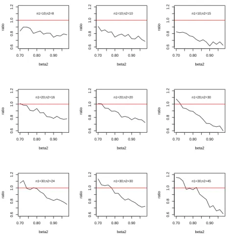
Example 1. The data are generated from models(8)withβ1=1andβ2=0.92. Let X1and X2

are independent and identically distributed with N(0, 1). Also, we set thatσ1 =σ2 =0.3. The

simulation study is conducted as follows. We consider three scenarios: (i) n₁<n₂; (ii) n₁=n₂; and (iii) n1>n2. The range of n1and n2is between 8 and 90. For each fixed sample size,1000

independent data sets are generated. Table 1 summarizes the results. It can be seen that both the MLE and WLE are close to the true values. The standard deviations of the WLE’s are consistently smaller than those of the MLE. Furthermore, the ratios of the MSE of the WLE to the MSE of the MLE are always smaller than 1. This implies that the WLE could reduce the MSE in contrast with the MLE. To assess the sensitivity of the ratio to actual value of the related parameterβ2, we run

simulations with differentβ2values ranging from0.7to0.98. The trend of the ratios against the

values ofβ2is provided in Figure 1. In general, we find that the smaller n1, the smaller the ratio

under the current setup. For each fixed n1, the ratios are inversely proportional to the value of

β2. They would also increase with larger value for n2. We see that the WLE outperforms the MLE

remarkably in small sample size n₁. This feature could be useful in practice if the first sample size is small and we have abundant related information.

0.70 0.80 0.90

0.6

0.8

1.0

1.2

beta2

ratio

n1=10;n2=8

0.70 0.80 0.90

0.6

0.8

1.0

1.2

beta2

ratio

n1=10;n2=10

0.70 0.80 0.90

0.6

0.8

1.0

1.2

beta2

ratio

n1=10;n2=15

0.70 0.80 0.90

0.6

0.8

1.0

1.2

beta2

ratio

n1=20;n2=16

0.70 0.80 0.90

0.6

0.8

1.0

1.2

beta2

ratio

n1=20;n2=20

0.70 0.80 0.90

0.6

0.8

1.0

1.2

beta2

ratio

n1=20;n2=30

0.70 0.80 0.90

0.6

0.8

1.0

1.2

beta2

ratio

n1=30;n2=24

0.70 0.80 0.90

0.6

0.8

1.0

1.2

beta2

ratio

n1=30;n2=30

0.70 0.80 0.90

0.6

0.8

1.0

1.2

beta2

ratio

n1=30;n2=45

Figure 1: The trend of the ratio values against β

2 for 9 ombinations of (n

u

o

,

X

.

W

a

n

g

,

Y.

W

u

/

E

u

r.

J.

P

u

re

A

p

p

l.

M

a

th

,

5

(2

0

1

2

),

3

3

3

-3

5

6

3

5

3

Table1: EstimatedvaluesbasedontheMLEandWLE,theorrespondingMSEandtheratiooftheMSE(WLE)totheMSE(MLE)forExample 1.

MLE WLE

n1 n2 βˆ(std) MSE(std) βˆ(std) MSE(std) λˆ(std) Ratio

10 8 1.009(0.239) 0.057(0.093) 0.997(0.21) 0.044(0.069) 0.744(0.187) 0.768

20 16 1.008(0.166) 0.028(0.041) 0.992(0.149) 0.022(0.033) 0.757(0.186) 0.807

30 24 1.006(0.128) 0.016(0.025) 0.993(0.113) 0.013(0.02) 0.754(0.188) 0.778

40 32 1.001(0.114) 0.013(0.019) 0.991(0.102) 0.01(0.016) 0.767(0.187) 0.813

50 40 1.005(0.098) 0.01(0.014) 0.994(0.09) 0.008(0.012) 0.781(0.194) 0.851

60 48 0.999(0.094) 0.009(0.013) 0.99(0.088) 0.008(0.012) 0.774(0.192) 0.875

10 10 1.004(0.241) 0.058(0.085) 0.985(0.206) 0.042(0.063) 0.742(0.186) 0.734

20 20 1.011(0.164) 0.027(0.04) 0.996(0.143) 0.02(0.032) 0.743(0.188) 0.751

30 30 1.003(0.134) 0.018(0.026) 0.989(0.117) 0.014(0.02) 0.758(0.188) 0.765

40 40 1.001(0.112) 0.013(0.018) 0.988(0.1) 0.01(0.015) 0.761(0.188) 0.808

50 50 0.994(0.099) 0.01(0.015) 0.981(0.088) 0.008(0.012) 0.764(0.189) 0.812

60 60 0.999(0.088) 0.008(0.011) 0.986(0.081) 0.007(0.009) 0.77(0.187) 0.867

10 15 0.986(0.249) 0.062(0.108) 0.966(0.196) 0.04(0.077) 0.717(0.181) 0.638

20 30 1.006(0.161) 0.026(0.039) 0.98(0.131) 0.017(0.026) 0.72(0.186) 0.675

30 45 0.995(0.13) 0.017(0.025) 0.977(0.106) 0.012(0.018) 0.74(0.184) 0.693

40 60 1.002(0.109) 0.012(0.017) 0.984(0.095) 0.009(0.014) 0.753(0.188) 0.78

50 75 1.002(0.101) 0.01(0.015) 0.982(0.084) 0.007(0.011) 0.754(0.184) 0.729

6. A Real Data Example

The low birth weight data comes from a study of risk factors associated with low infant birth weight.The data were collected at Baystate Medical Center, Springfield, Massachusetts, during 1986 and presented in[8]. The goal of this study was to identify risk factors associated with giving birth to a low birth weight baby who weighs less than 2500 grams. In this study data were collected on 189 women, 59 of which had low birth weight babies and 130 of which had normal birth weight babies. Variables which were thought to be of importance were weight of the subject at her last menstrual period and race. These two variables are denoted as "LWT" and "RACE". The response "LOW", is a binary variable which indicates a low birth weight baby if equals to 1, and normal birth weight if equals to 0. The variable "RACE" has been recoded using the two dummy variables. First of all, we investigate on the model

g(µ) =β0+β1LW T,

whereµ is the expected value of the binary response and g is the link function for binomial family. We find that the variable LWT is significant. The estimate of the coefficients and the corresponding p-values are given in Table 2. One can also verify that the interaction between LWT and RACE is not significant.

Table2: EstimatedCoeientsforgenerallogistiregressionmodelusingthevariablesLWT. Estimate p-value

Intercept 0.9983 0.2036 LWT -0.0141 0.0227

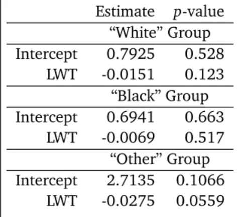
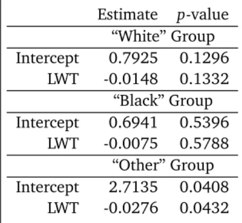
Then we check the significance of LWT within each RACE individually. The p-values are all greater than the p-value of LWT for each group is given in Table 3. Despite the fact that the variable LWT is significant for the overall model, it is very surprising to see that the LWT is not significant within any group. By applying the WLE method based on distribution from bootstraping, we find the LWT is significant in "Other" group.

Table3: EstimatedCoeientsforgenerallogistiregressionmodelusingthevariablesLWTineahRACE group.

Estimate p-value “White” Group Intercept 0.7925 0.528

LWT -0.0151 0.123 “Black” Group Intercept 0.6941 0.663

LWT -0.0069 0.517 “Other” Group Intercept 2.7135 0.1066

Table4: Estimated Coeientsforweightedlogistiregressionmodelusingthevariables LWTwitheah RACEgroupasthemaingroup. P-valuesarebasedonbootstrapdistribution.

Estimate p-value “White” Group Intercept 0.7925 0.1296

LWT -0.0148 0.1332 “Black” Group Intercept 0.6941 0.5396

LWT -0.0075 0.5788 “Other” Group Intercept 2.7135 0.0408

LWT -0.0276 0.0432

7. Discussion

To obtain a more efficient estimator with a smaller MSE when related information is avail-able, we proposed the weighted likelihood inference for the parameters in linear and par-tially linear models. We developed a data-driven approach to estimate the weights to address the vexing issued in weighted likelihood inference. The proposed estimators have the same asymptotically normal distribution as the maximum likelihood estimators. The advantage of the WLE over the classical MLE was illustrated by simulation studies. Results from these simu-lation studies suggest that the proposed estimators have prospective promises. The simplicity and effectiveness of the proposed adaptive weights are also appealing.

We remark that the real data set used in this paper actually came from a longitudinal study. Thus one must recognize the within-subject and between-subject variations. Further investigation of the inference based on the weighted likelihood for mixed-effect models is required.

ACKNOWLEDGEMENTS The research was partially supported by the Natural Sciences and Engineering Research Council of Canada.

References

[1] J Shao.Mathematical Statistics. Springer, New York, 2003.

[2] J Staniswalis. The kernel estimate of a regression function in a likelihood-based models. J. Am. Statist. Assoc., 84:276–83, 1989.

[3] M Stone. Strong inconsistencies from uniform priors.J. Am. Statist. Assoc., 71:114–116, 1976.