Unsupervised Dimensionality Reduction for High-Dimensional Data Classification

http://www.sciencepublishinggroup.com/j/mlr doi: 10.11648/j.mlr.20170204.13

Unsupervised Dimensionality Reduction for

High-Dimensional Data Classification

Hany Yan

*

, Hu Tianyu

School of Mathematics, Jilin University, Changchun, China

Email address:

[email protected] (Han Yan), [email protected] (Hu Tianyu) *

Corresponding author

To cite this article:

Hany Yan, Hu Tianyu. Unsupervised Dimensionality Reduction for High-Dimensional Data Classification. Machine Learning Research. Vol. 2, No. 4, 2017, pp. 125-132. doi: 10.11648/j.mlr.20170204.13

Received: July 20, 2017; Accepted: August 9, 2017; Published:August 31, 2017

Abstract:

This paper carries on research surrounding the influences produced by dimensionality reduction on machine learning classification effect. Firstly, paper constructs the analysis architecture of data dimension reduction classification, combines the two different unsupervised dimension reduction methods, locally linear embedding (LLE) and principal component analysis (PCA) with the five machine learning classification methods: Gradient Boosting Decision Tree (GBDT), Random Forest, Support Vector Machine (SVM), K-Nearest Neighbor (KNN) and Logistic Regression. And then uses the handwritten digital identification dataset to analyze the classification performance of these five classification methods on different dimension datasets by different dimensionality reduction methods. The analysis shows that using the appropriate dimensionality reduction method for dimensionality reduction classification can effectively improve the classification accuracy; the dimensionality reduction classification effect of non-linear dimensionality reduction method is generally better than the linear dimensionality reduction method; different machine learning classification algorithms have significant differences in the sensitivity of dimensions.

Keywords: Dimensionality Reduction, Machine Learning, Classification Problem, Handwritten Numeral Recognition

1. Introduction

With rapid advances in science and technology nowadays, the marginal cost associated with data collection is decreasing, and more and more big data of different types are available for scientific analysis. In the context of data explosion, however, high data dimensionality occurs, posing considerable challenges to classification. The traditional classification algorithms rely on distance or density of data items. But in the case of high dimensionality, these methods are not effective anymore due to space sparsity. Moreover, directly classifying high-dimensionality data using the classification methods causes heavy time costs and computational complexities. This limits the widespread application of the traditional classification algorithms.

From the perspective of machine learning, the classification can be regarded as a supervised learning method where the training dataset is used to establish paradigm and output feature of the prediction set [1]. Because most of existing data have high dimensionality,

type of method and reported that most of the existing machine learning and data mining methods are ineffective to high-dimensionality data. The accuracy of machine learning-based classification decreases quickly with data dimensionality. Training data after dimensionality reduction can make full use of fewer features more effectively and thus avoid over-fitting.

Therefore, reducing data dimensionality is critical to the classification of high-dimensionality data through machine learning. It is of great significance to study dimensionality reduction based classification of high-dimensionality data.

2. Overview of Dimensionality Reduction

The dimensionality reduction technology is designed to reduce the dimensionality of raw data. It is very important to data mining and machine learning. By reducing the number of data features, it can considerably improve the classifier’s performance and reduce computational loads [8].

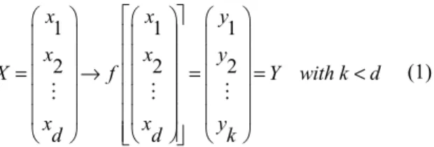
Feature extraction is an important idea for dimensionality reduction, where information is extracted from existing samples to produce new feature variables, also known as second-order features. The main aim of feature extraction is to replace original high-dimensionality features with fewer low-dimensionality more effective ones [9], as shown in the following equation.

1 1 1

2 2 2

 

     

 

     

 

     

= →  = = <

 

     

 

     

 

     

⋮ ⋮ ⋮

x x y

x x y

X f Y with k d

x x y

d d k

(1)

If the second-order features are combined linearly during feature extraction, it is called linear dimensionality reduction. Otherwise, it is called non-linear dimensionality reduction.

Linear dimensionality reduction belongs to the traditional field of statistics and applied mathematical research. The typical algorithms of linear dimensionality reduction are principal component analysis [10], linear discriminant analysis and [11] multi-scale transformation [12] and so on. Their commonality is that the original data set is embedded in a global linear structure. Because the linear model is simple to calculate, it has a good effect for the data with a linear structure or Gaussian distribution, but in the real circumstances, the data structure may be non-linear to fail to extract the geometric structure, the effect of dimensionality reduction will be compromised.

Based on the shortcomings of linear dimensionality reduction, the non-linear dimensionality reduction methods have been paid more and more attention. The early non-linear dimensionality reduction methods were mainly based on kernel method, in which the data with non-linear features were mapped into the high-dimensional space through the kernel method, and the linear dimensionality reduction method was used in that high dimension space. One of the typical methods under this idea is kernel principal component

analysis [12]. But this method also has a shortcoming that cannot be ignored, that is the choice of the most critical core is very difficult and can only rely on experience to judge. In recent years, manifold learning, as another non-linear dimensionality reduction idea, has become more and more important in the eyes of people due to the limitations of kernel-based dimensionality reduction, the typical algorithms are local linear embedding [13] and isometric mapping [14]. The common idea of this kind of non-linear dimensionality is to observe the initial feature structure in the high-dimensional space of the data, and then to establish the mapping from high dimension to low dimension, so that the specific information of data can be kept in the lower dimension. The manifold-based dimensionality reduction method is verified to be often more efficient than the kernel-based method in the processing of high-dimensional data with non-linear structures [15].

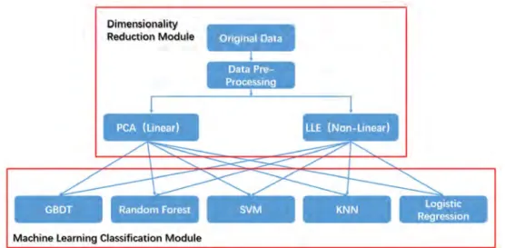
It can be seen from Figure 1 that many dimensionality reduction methods are available currently. Among various linear algorithms, PCA is easy, parameter-free and thus widely used in different scenarios [16]. Among various non-linear algorithms, LLE is a classic unsupervised non-non-linear method, which transforms the global non-linear structure into a local linear structure. The data is converted into low-dimensional through linear embedding. In this way, computational complexity is considerably reduced and high-dimensional space structure is maintained [17]. PCA and LLE are selected as the representative of the linear and non-linear algorithms to study the influence of unsupervised dimensionality reduction on data classification.

Figure 1. Classification of Dimensionality Reduction Methods.

2.1. Principal Component Analysis (PCA)

The main idea of PCA is to perform a linear transformation on original features, find out new non-correlated features, sort them in descending order of importance, and then represent data with fewer principal components. It is a typical unsupervised linear method for dimensionality reduction. Its major steps are given below.

i. Data standardization

Data standardization involves calculation of the data’s variance and mean.

var( )

j j

s = x (2)

the mean: 1 1 n j ij i x x n =

=

∑

(3)

and the canonical transformation:

ij j ij j x x X s −

= (4)

ii. Calculation of correlation coefficient matrix

The correlation coefficient matrix of the standardized data can be computed as:

11 12 1 12 1

21 22 2 21 2

1 2 1 2

1 1 ( ) 1 p p p p

p p pp p p

r r r r r

r r r r r

R Cov X

r r r r r

            = =_{  }= _             ⋯ ⋯ ⋯ ⋯ ⋮ ⋮ ⋮ ⋮ ⋮ ⋮ ⋮ ⋮ ⋯ ⋯ (5) where 1 2 2 1 1 ( )( ) ( ) ( ) n

ki i kj j

k

ij _{n n}

ki i kj j

k k

x x x x

r

x x x x

= = = − − = − −

∑

∑

∑

(6) Let

1 2 p

λ λ≥ ≥⋯λ ≥ 0 (7)

denote the feature values of the correlation coefficient matrix

R. and

1, 2, p

a a ⋯a (8)

denote the feature vectors. The orthogonal matrix:

' 1 2

( , , _p),

A= a a ⋯a AA =I (9)

the principal components:

' 1 2

( , , _p)

Z = Z Z ⋯Z (10)

Where

'

i i

Z =a X (11)

Hence, the correlation coefficient matrix can be written as:

11 12 1 1 11 21 1

21 22 2 2 12 22 2

1 2 1 2

p p

p p

p p pp p p p pp

a a a a a a

a a a a a a

R

a a a a a a

λ λ λ                   =_{     }                   ⋯ ⋯ ⋯ ⋯ ⋮ ⋮ ⋮ ⋮ ⋱ ⋮ ⋮ ⋮ ⋮ ⋯ ⋯ (12)

iii. Choice of principal component based on contribution The contribution of the component is defined as the ratio

of its feature value to the sum of all feature values.

1 i i p i i Contribution λ λ = =

∑

(13)

Because the components’ variance decreases gradually, p

components will be obtained during the process of PCA. Generally, the top few components whose cumulative contribution exceeds a threshold (80%) [18] are selected in practical applications. The cumulative contribution of the top m components is:

1 1 R m i i p i i Cumulative ate λ λ = = =

∑

∑

(14)

2.2. Local Linear Embedding (LLE)

Local linear embedding is an unsupervised non-linear dimensionality reduction method based on manifold learning. It can transform global non-linear structure into local linear structure. By locally reconstructing matrix of weights, it can reduce dimensionality while maintaining high-dimensionality space structure. Its main steps are described as follows.

i. Calculate distance from proximal point in the high-dimensionality space

The distance between each sample xiin the original

high-dimensionality data and its neighbors is computed. And k

points are chosen as the proximal points, where k<N. The distance is computed as:

2

( )

ij ik jk

d =

∑

x −x (15)

ii. Calculate locally reconstructed weight matrix First, the error function is defined as:

2

1 1

min ( )

N k

i ij ij

i j

W x w x

ε

= =

=

∑

−

∑

(16)

where xij (j = 1, 2,…, k) denotes the k proximal points of xij,

wijis the weight and:

1 1 k ij j w = =

∑

(17)

For any point xij, its error is:

2 2

1 1 1 1

( )

k k k k

i

i ij ij ij i j ij im jm

j j j m

x w x w x x w w Q

ε

= = = =

= −

∑

=

∑

− =

∑∑

(18)

where:

( ) ( )

jm

i T

i j i m

Q = x −x x −x (19)

the locally reconstructed weight matrix:

1 1

1 1 1

( )

( ) k

i jm m ij k k

i pq p q

Q w

Q

− =

− = =

=

∑

∑∑

(20)

When Qiis a singular matrix, it can be regularized as:

i i

Q =Q +rI (21)

where r denotes regularization parameter, and I denotes identity matrix.

iii. Search for low-dimensionality space mapping

The samples xiand xj in the high-dimensionality space are

projected to yi and yi in the low-dimensionality space. Due to

the need to maintain local structure of the high-dimensionality space, the weight matrix wij remains the same

and the mapping objective function is:

2

1 1

min ( )

N k N N

T

i ij ij ij i j

i j i j

Y y w y M y y

ε

= =

=

∑

−

∑

=

∑∑

(22)

subject to:

1

1

0

1

N

i i

N T i i i

y

y y I

N =

= 

=

  

 ₌



∑

∑

(23)

The matrix M in the objective function is a N*N symmetric matrix.

( ) (T )

M = −I W I W− (24)

The method of Lagrange multipliers can be used to obtain:

T T

MY =

λ

Y (25)

In order to minimize the objective function, Y is set to the feature vector corresponding to the minimal vector value of

M. After sorting the feature vectors of M in ascending order of feature value, the feature vectors corresponding to 2~d+1

are usually selected for low-dimensionality embedding.

3. Dimensionality Reduction

Classification for Handwritten Digit

Recognition

3.1. Data Description

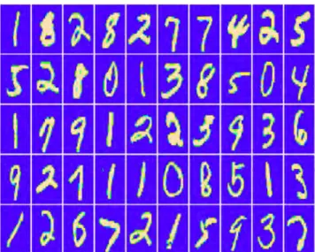
The handwritten digit recognition technology is designed to recognize the handwritten Arabic numerals in the paper or image using the recognition methods. In this paper, handwritten digit recognition is studied using the handwritten digit dataset MNIST [19], which stores 42,000 785-dimension 28*28 images of handwritten digit.

Figure 2. Handwritten Number Image data.

Figure 3. The Difference of Handwritten Number.

Figure 4. Data Distribution.

3.2. Analysis Structure

Figure 5. The Analysis Structure of Dimensionality Reduction Classification.

Two dimensionality reduction methods and five machine learning classification algorithms are used in this paper. A lot of parameter and model settings need to be selected during implementation, including the choice of the kernel function and penalty factor C for SVM, the choice of k for KNN and LEE, as well as the number of iterations, step length and loss function for GBDT. These settings are selected in a way that can maximize algorithm performance.

Mathematical forms and more details of these machine learning classification algorithms are available in [20] [21] [22] [23] [24] [25].

In order to evaluate the performance of machine learning-based classification methods for different dimensions, the training and test datasets are partitioned through the k-fold (k = 5) cross-validation approach [26], as shown in the following figure.

Figure 6. k-Fold Cross-Validation.

The figure above is variance explained by top 100 components by PCA, it can be seen that the top 10 of the 100 components have made over 80% contributions in total, the top 25 components made over 95% contributions, and the top 50-100 components made over 97% contributions stably. Therefore, the original data is reduced to 100, 50, 25 and 10 dimensions using PCA and LLE, respectively. Afterward, the five machine learning-based classification algorithms are compared on each of the four datasets whose dimensionality is reduced using the k-fold cross validation approach.

Dimensionality reduction and classification methods are implemented in this paper using the toolbox of R, Python and Spark. The packages and libraries used for algorithm implementation include caret, scikit-learn, XGBoost and MLlib.

3.3. Result Analysis

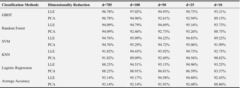
The final results of dimensionality reduction and classification results are shown in the following table.

Table 1. The Prediction Accuracy in Different Dimensionality Reduction Classification Methods.

Classification Methods Dimensionality Reduction d=785 d=100 d=50 d=25 d=10

GBDT LLE 96.78% 97.02% 94.93% 94.73% 93.21%

PCA 96.78% 94.96% 92.61% 92.94% 89.15%

Random Forest LLE 94.09% 94.79% 94.69% 95.16% 93.73%

PCA 94.09% 92.46% 92.73% 93.26% 88.75%

SVM LLE 94.76% 95.09% 94.22% 94.83% 89.22%

PCA 94.76% 95.29% 94.72% 95.06% 91.99%

KNN LLE 91.82% 94.43% 93.92% 94.73% 92.75%

PCA 91.82% 89.09% 92.69% 94.56% 90.82%

Logistic Regression LLE 88.23% 94.51% 95.15% 94.96% 93.25%

PCA 88.23% 88.91% 86.81% 86.59% 83.57%

Average Accuracy LLE 93.14% 95.17% 94.58% 94.88% 92.43%

PCA 93.14% 92.14% 91.91% 92.48% 88.86%

Generally speaking, the average classification accuracy of the linear PCA method is inferior to that of the non-linear LLE method. This is mainly because the handwritten digit has geometric features, and LLE can reduce dimensionality while maintaining space structure of the high-dimensionality data.

Figure 8. The Average Classification Accuracy of LLE and PCA.

Although LLE is superior to PCA in terms of average classification accuracy, the five machine learning algorithms differ greatly in classification accuracy.

Figure 9. The Classification Accuracy of GBDT with Different Dimensionality Reduction Methods.

interference effectively. It may also be the main reason why GBDT performs well on the raw dataset but the accuracy benefits slightly from dimensionality reduction.

Figure 10. The Classification Accuracy of Random Forest with Different Dimensionality Reduction Methods.

Like GBDT, Random Forest is also an ensemble machine learning method based on decision tree. Its performance resembles GBDT very much. The baseline classification accuracy of the Random Forest method is 94.09%, and it reaches its greatest level of 95.16% on the dataset whose dimensionality is reduced to 25 dimensions by LLE, higher than the baseline by 1.07%. But in the case of dimensionality reduction through PCA, none of the four dimensions obtains an accuracy higher than the baseline.

Figure 11. The Classification Accuracy of SVM with Different Dimensionality Reduction Methods.

The baseline accuracy of SVM is 94.76%, and it reaches its highest level of 95.09% in the case of LLE-based dimensionality reduction. Moreover, its highest level of accuracy in the case of LLE-based dimensionality reduction is almost the same as that in the case of PCA-based dimensionality reduction. Because the Gaussian kernel is adopted to train SVM, it can classify high-dimensionality data through non-linear mapping. Hence, it is not sensitive to data dimensionality and its classification accuracy does not benefit a lot from dimensionality reduction.

Figure 12. The Classification Accuracy of KNN with Different Dimensionality Reduction Methods.

The baseline accuracy of KNN is 91.82%. Note that its greatest accuracy is reached when the dataset is reduced to 25 dimensions, irrespective of dimensionality reduction methods. The original dimensionality of the data is reduced by nearly 97% from 784 to 25, indicating the considerable sensitivity of KNN to dimensionality. The spatial neighborhood is determined while training KNN, and the sparsity of high-dimensionality data usually reduces the reliability of this method. Therefore, the classification accuracy of KNN benefits a lot from appropriate dimensionality reduction.

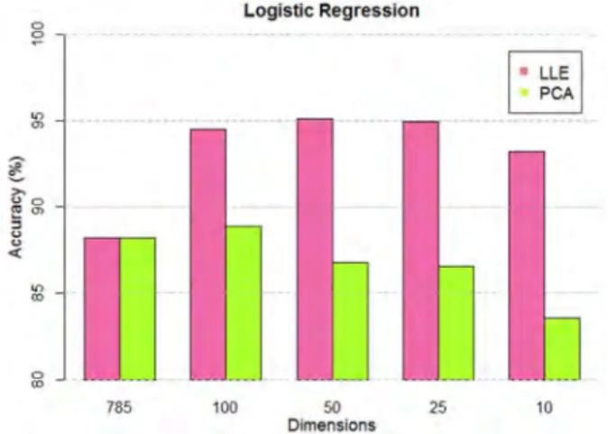
Figure 13. The Classification Accuracy of Logistic Regression with Different Dimensionality Reduction Methods.

The baseline accuracy of the Logistic regression method is merely 88.23%, the lowest among the five algorithms. Its greatest accuracy is 95.15%, higher than the baseline by 6.92%. The increment is larger than any other method. From this, it can be seen that data dimensionality and noise has an enormous impact on the classification accuracy of the Logistic regression method.

4. Conclusion

work has been done to study the variation of the machine learning classification algorithms with different dimensionality reduction methods and different dimensionalities. This paper focuses on the influence of unsupervised dimensionality reduction on machine learning-based classification of high-dimensional data. Data dimensionality is first reduced using linear and non-linear methods. The performance of several machine learning algorithms to classify the data with varying dimensionality is then compared. The following conclusion is reached and it is expected to produce useful insights into existing work. First, classification accuracy can be increased effectively by performing appropriate dimensionality reduction before training. But over-reduction of dimensionality may result in a dramatic decline in classification accuracy. Second, results of the experiment on handwritten digit indicate that the non-linear dimensionality reduction method like LLE is more beneficial to classification performance than the linear dimensionality reduction method like PCA, given the set of data with clear geometric structures. Finally, the sensitivity of classification performance to dimensionality varies among the machine learning-based classification algorithms. For example, the decision tree-based approaches (GBDT and Random Forest) and the kernel-based approaches (SVM) are able to choose appropriate features and resist noise. Therefore, these methods are insensitive to data dimensionality, and their classification accuracy reaps few benefits from dimensionality reduction. But the simple machine learning algorithms like Logistic regression and KNN are very sensitive to data dimensionality and noise.

References

[1] Gaber, Mohamed Medhat, A. Zaslavsky, and S. Krishnaswamy. A Survey of Classification Methods in Data Streams. Data Streams. 2015:39-59.

[2] Su, Jiang, and H. Zhang. "A fast decision tree learning algorithm." National Conference on Artificial Intelligence AAAI Press, 2006:500-505.

[3] Serpen, Gursel, and S. Pathical. "Classification in High-Dimensional Feature Spaces: Random Subsample Ensemble." International Conference on Machine Learning and Applications 2009:740-745.

[4] Fan, J., and Y. Fan. "High Dimensional Classification Using Features Annealed Independence Rules." Annals of Statistics 36.6(2008):2605.

[5] Miller, Alan. Subset selection in regression. Chapman & Hill/CRC, 2002.

[6] Fodor, I. K. "A survey of dimension reduction techniques." Neoplasia 7.5(2002):475-485.

[7] Mitchell, Tom M., J. G. Carbonell, and R. S. Michalski. Machine Learning. McGraw-Hill, 2003.

[8] Huang, Cheng Lung, and J. F. Dun. "A distributed PSO–SVM hybrid system with feature selection and parameter optimization." Applied Soft Computing 8.4(2008):1381-1391.

[9] Tsai, Flora S., and K. L. Chan. "Dimensionality reduction techniques for data exploration." International Conference on Information, Communications & Signal Processing IEEE, 2007:1-5.

[10] Hotelling, H. H. "Analysis of Complex Statistical Variables into Principal Components." British Journal of Educational Psychology 24.6(1933):417-520.

[11] Zigelman, G, R. Kimmel, and N. Kiryati. "Texture mapping using surface flattening via multi-dimensional scaling." IEEE Transactions on Visualization and Computer Graphics 2002:198-207.

[12] Kuang, Fangjun, W. Xu, and S. Zhang. "A novel hybrid KPCA and SVM with GA model for intrusion detection." Applied Soft Computing 18. C(2014):178-184.

[13] Bengio, Yoshua, et al. "Out-of-sample extensions for LLE, Isomap, MDS, Eigenmaps, and Spectral Clustering." International Conference on Neural Information Processing Systems MIT Press, 2003:177-184.

[14] Balasubramanian, M, and E. L. Schwartz. "The isomap algorithm and topological stability." Science 295.5552(2002):7. [15] Gorban, Alexander N., et al. Principal Manifolds for Data

Visualization and Dimension Reduction. Springer Berlin Heidelberg, 2008.

[16] Moore, B. "Principal component analysis in linear systems: Controllability, observability, and model reduction." IEEE Transactions on Automatic Control 26.1(2003):17-32.

[17] Wang, Jianzhong. Locally Linear Embedding. Geometric Structure of High-Dimensional Data and Dimensionality Reduction. Springer Berlin Heidelberg, 2012:203-220.

[18] Egeren, Lawrence F. Multivariate Statistical Analysis. North-Holland Pub. Co, 1973.

[19] Kussul, Ernst, and T. Baidyk. "Improved method of handwritten digit recognition tested on MNIST database." Image & Vision Computing 22.12(2004):971-981.

[20] Xie, Keming, C. Mou, and G. Xie. "The multi-parameter combination mind-evolutionary-based machine learning and its application." 1.1(2000):183-187 vol.1.

[21] Burges, Christopher J. C. A Tutorial on Support Vector Machines for Pattern Recognition. Kluwer Academic Publishers, 1998.

[22] Dietterich, Thomas G. "An Experimental Comparison of Three Methods for Constructing Ensembles of Decision Trees: Bagging, Boosting, and Randomization." Machine Learning 40.2(2000):139-157.

[23] Song, Yang, et al. IKNN: Informative K-Nearest Neighbor Pattern Classification. Knowledge Discovery in Databases: PKDD 2007. Springer Berlin Heidelberg, 2007:248-264.

[24] Andrew Cucchiara. "Applied Logistic Regression." Technometrics 34.1(1992):358-359.

[25] Cutler, Adele, D. R. Cutler, and J. R. Stevens. "Random Forests." Machine Learning 45.1(2012):157-176.