Vol. 12, No. 4, 2019, 1360-1370 ISSN 1307-5543 – www.ejpam.com Published by New York Business Global
Optimal Solution Properties of an Overdetermined
System of Linear Equations
Vedran Novoselac1,∗, Zlatko Pavi´c 1
1 Mechanical Engineering Faculty in Slavonski Brod, University of Osijek,
Trg Ivane Brli´c Maˇzurani´c 2, 35000 Slavonski Brod, Croatia
Abstract. The paper considers the solution properties of an overdetermined system of linear equations in a given norm. The problem is observed as a minimization of the corresponding functional of the errors. Presenting the main results of p norm it is shown that the functional is convex. Following the convex properties we examine minimization properties showing that the problem possesses regression, scale, and affine equivariant properties. As an example we illustrated the problem of finding the weighted mean and weighted median of the data.
2010 Mathematics Subject Classifications: 15A06, 65F20, 58K70
Key Words and Phrases: Linear equations, overdetermined systems, equivariance
1. Introduction
A system of linear equations denoted as Ax=b where
A=
a11 . . . a1n
..
. ... ... am1 . . . amn
∈R
m×n, x=
x1 .. . xn
∈R
n, b=
b1 .. . bm
∈R
m. (1)
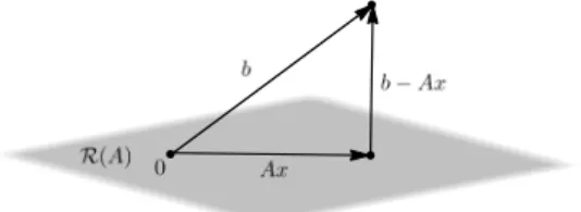
If A is m×n matrix, with m > n, then it is said that the linear system of equations is overdetermined. In general, such a system will have no solution, i.e. it is inconsistent, i.e. b /∈ R(A). Instead the solution with the smallest error kb−Axkp is observed using some p∈[1,∞inorme, where the problem is to find a vector x∈Rn such that
min
x∈Rn
kb−Axkp, p∈[1,∞i. (2) Figure 1 presents the problem of an overdetermined system of linear equations.
∗
Corresponding author.
DOI: https://doi.org/10.29020/nybg.ejpam.v12i4.3517
Email addresses: [email protected](V. Novoselac),[email protected](Z. Pavi´c)
Figure 1: Graphic illustration of an overdetermined systemAx=b.
Problem (2) can be observed as a minimization problem of a functional
fp(x) =kb−Axkp =
m
X
i=1 |bi−
n
X
j=1 aijxj|p
1 p
, p∈[1,∞i. (3)
Many problems can be presented as an overdetermined system of linear equations such as the problem of determinating linear models for fitting experimental data. It is intended to help researchers fit appropriate curves to their data. Curve fitting, also known as regression analysis, is a common technique for modelling data [13]. The problem of determining n-dimensional hyperplane, in order to have its graph pass as close as possible to given points in sense ofpnorme, can be presented as an overdetermined system of linear equations [2]. In linear regression analysis it is most frequently assumed that errors, i.e. so called ’outliers’, can occur in measured values of the independent variable. In this case, if Eu-clidian norm (p= 2) is used, vectorx∈Rnis obtained in the sense of Least Squares (LS)
problem by minimizing (3). In many technical and other applications using the p = 1 norm is much more interesting. Because of robust properties of p = 1 norm the outliers in data should not affect the obtained results. In literature this problem is known as the Least Absolute Deviation (LAD) problem, and is an efficient method for outlier detection [11, 14].
For that purpose some properties of functional fp:Rn → R are shown in Section 2,
especially taking into account the equivariant properties of a solution of an overdetermined system of linear equations. In Section 3, we analyzed equivariant properties of the weighted mean and weighted median of the data, which are a reduced case of an overdetermined system of linear equations, where p= 1, p= 2 is observed, andn= 1 respectively.
2. Properties of the Functional fp
In this section we present some properties of functional fp:Rn→Rin order to prove
equivariant properties. Following the Minkowski inequality presented in Theorem 9, which is proven in Section 5, presented in appendix, we give directly the next theorem.
Theorem 1. Functional fp:Rn→R is convex onRn.
for differentiable functions, because it is not always possible to solve ∇fp(x) = 0 to
calculate critical points. In the situation when p = 2, the problem is known as the LS problem and it always has a solution. In this casex∗ minimizesf2 if and only ifx∗ solves normal equation system ATAx= ATb. It can be shown that if A ∈
Rm×n has full rank
n, then the LS problem has a unique minimizer. In that case global extremum can be presented as x∗ = A+b, where matrix A+ = (ATA)−1AT is usually called the Moore-Penrose inverse [3]. In most general cases, convex functionalfp has a particularly simple
extremal structure, and there are algorithms to calculate extremum points, supposing its existance [15]. Knowing whether or not a local minimum is also global, is one of the most important questions in optimization [7]. The assumption of convexity gives a positive answer to this question as it is stated in the following theorem.
Theorem 2. A local minimumx∗of a functionalfp:Rn→Ris always a global extremum.
Proof. Suppose thatx∗is a local minimum offp, that is, there is an open neighborhood
U ofx∗wherefp(x∗)≤fp(x),∀x∈U.We prove thatfp(x∗)≤fp(y∗) for arbitraryy∗ ∈Rn.
Consider the convex combination (1−λ)x∗+λy∗, for λ∈[0,1], the convex combination approaches to x∗ as λ → 0. Therefore for small enough λ, (1−λ)x∗ +λy∗ is in the neighborhood U. Then
fp(x∗) ≤ fp((1−λ)x∗+λy∗)
≤ (1−λ)fp(x∗) +λfp(y∗).
(4)
Rearranging terms, we havefp(x∗)≤fp(y∗).
From the Theorem 2, it directly follows that the local minimum of a convex functional is necessarily the global minimum. However, this minimum is not necessarily unique, a sufficient condition is strict convexity. Let us now discuss some equivariant properties of functional fp. We considered three types of equivariance: regression, scale, and affine
equivariance [11]. The next theorem shows that functionalfp possesses these three types
of equvivarance.
Theorem 3. Let A∈Rm×n, m > n, b∈
Rm, and x∗∈Rn such that
fp(x∗) = min
x∈Rnkb−Axkp, p∈[1,∞i. (5) Then
(a) For an arbitrary v∈Rn, vector x∗+v is a solution of
min
x∈Rnkb+Av−Axkp. (6) (b) For any c∈R, vector c x∗ is a solution of
min
x∈Rn
(c) For a nonsingular matrixB ∈Rn×n, vector B−1x∗ is a solution of
min
x∈Rnkb−ABxkp. (8) Proof. Let us discuss:
(a) Lety∗ be a solution of (6). Then
kb+Av−Ay∗kp =kb−A(y∗−v)kp ≥ kb−Ax∗kp, (9)
whereby the equation is only ify∗−v=x∗.
(b) For c= 0 the assertion is obvious. Let c6= 0, and y∗ such that is a solution of (7). Then
kcb−Ay∗kp =|c|
b−A
y∗ c
p
≥ |c|kb−Ax∗kp, (10)
whereby the equation is only if yc∗ =x∗. (c) Lety∗ be a solution of (8). Then
kb−ABy∗kp ≥ kb−Ax∗kp, (11) whereby the equation is only ifBy∗=x∗.
Corollary 1. Let A∈Rm×n, m > n, b∈
Rm, andx∗∈Rn such that
fp(x∗) = min x∈Rn
kb−Axkp, p∈[1,∞i. (12)
Then for an arbitrary v ∈ Rn, c ∈
R, and nonsingular matrix B ∈ Rn×n, vector
cB−1(x∗+v) is a solution of
min
x∈Rn
kc(b+Av)−ABxkp. (13)
3. Weighted Mean and Weighted Median of the Data
In this section we will illustrate the equivariant properties of the weighted mean and weighted median of the data. As we mentioned, the problem of the weighted mean and weighted median are essentially reduced to solving an overdetermined system of linear equations. Numerous applications of this problem can be found in various branches of applied research, like image processing [10], or methods for outlier detection [11].
Let a ∈ Rm be the vector data with corresponding positive vector data weights
w∈Rm
+. If we denote by A = [p √
w1, . . . , p √
wm]T and b = [p
√
w1a1, . . . , p √
wmam]T in
functionfp:R→R, wheren= 1, then follows that
f2(x) =kb−Axk2=
v u u t
m
X
i=1
is convex and attains its global minimum on the set R, which is denoted by
x∗ = mean(w, a) and called the weighted mean of the data. If w1 = · · · = wm = 1, the global minimum of the corresponding functional (14) is
de-noted by x∗ = mean(a) and called the mean of the data. Analogously, a real number which minimizes function
f1(x) =kb−Axk1=
m
X
i=1
wi|ai−x|, (15)
is called the weighted median of the data and is denoted by x∗= med(w, a). If w1=· · ·=wm = 1, the global minimum of the corresponding function (15) is denoted by
x∗ = med(a) and called the median of the data. In the Figure 2 we present the example of function fp, for p = 2 and p = 1 norm. Functions are generated with data vector
a= [1,2,3,4,5]T and corresponding weights vector w= [1,1,2,1,1]T presented in Figure 2(a) for p = 2, and for p=1 in Figure 2(b). In Theorem 4 it is shown that the minimum of the function f2, i.e. weighted mean, always achieved unique minimum. Considering the different data weightsw= [1,3,2,1,1]T, presented in Figure 2(c), it can be seen that the construction of the minimum of f1, i.e. weighted median, directly depends on it, and achieved its minimum on interval [a(2), a(3)], in contrast to the situation in Figure 2(b) where the minimum is unique. Also, it can be seen that function f1 is a piecewise linear function. This property of functionalf1is considered for finding a minimum, where details are presented in Theorem 5. In the sequel we give solutions for minimizing problems (14) and (15), i.e. for the weighted mean and weighted median of the data.
2 4 6 8
y
x f2
x∗= mean(w, a)
5 10 15 20
y
x f1
a(1)a(2) a(3) a(4) a(5) 5 10 15 20 25
y
x f1
a(1)a(2) a(3) a(4) a(5)
(a) (b) (c)
Figure 2: Functionfp:R→R.
Theorem 4. Let a ∈ Rm, m ≥ 2, be the data vector with corresponding data weights
w∈Rm
+. Then
mean(w, a) = 1 W
m
X
i=1
wiai, W = m
X
i=1
wi. (16)
Proof. Because the functional defined by (14) is derivable, the minimum is attained by finding a solution of ∂f2(x)
Corollary 2. Let a∈Rm, m≥2, be the data vector, then
mean(a) = 1 m
m
X
i=1
ai. (17)
Theorem 5. Let a ∈ Rm, m ≥ 2, be the data vector with corresponding data weights
w∈Rm
+. Let a(1)≤a(2) ≤. . .≤a(m) denote ordered observation and 0< w(1)≤w(2) ≤. . .≤w(m) corresponding weights. Thereby with the denotation
L:=
n
l:
l
X
i=1 w(i)≤
W 2
o
, l∈ {1, . . . , m}, W =
m
X
i=1
wi, (18)
(a) if L=∅, then med(w, a) =a(1);
(b) if L 6=∅, then with the denotation l0 = maxL there holds: (i) if
l0 P
i=1
w(i)< W2 , then med(w, a) =a(l0+1);
(ii) if
l0 P
i=1
w(i)= W2 , then med(w, a)∈[a(l0), a(l0+1)]. Proof. Notice that on each interval
h−∞, a(1)i,ha(1), a(2)i, . . . ,ha(m−1), a(m)i,ha(m),∞i,
functionf1: R→R defined by (15) is linear, and thereby derivable. The slopes of those
linear functions are consecutivelykl,l= 0, . . . , m, where
k0=−
m
X
i=1
wi, km= m
X
i=1
wi (19)
and for l= 1, . . . , m−1
kl= 2 l
X
i=1 w(i)−
m
X
i=1
wi=kl−1+ 2w(l). (20)
If L=∅, then for everyl= 1, . . . , m−1, is k0 <0< kl. It follows that f1 is strongly decreasing on h−∞, a(1)i and strongly increasing onha(1),∞i, therefore the minimum of f1 is attained forx∗ =a(1).
If L 6=∅, thenkl+1−kl = 2w(l+1)>0, and the sequence (kl) is increasing and
k0 < k1<· · ·< kl0 ≤0< kl0+1 <· · ·< km. (21)
If k(l0)<0, it follows from (21) that f1 is decreasing onh−∞, a(l0+1)i and increasing
on ha(l0+1),∞i, therefore the minimum off1 is attained forx ∗ =a
If k(l0) = 0, it follows from (21) that f1 is decreasing on h−∞, a(l0)i, is constant on
[a(l0), a(l0)+1] and increasing on ha(l0+1),∞i, therefore the minimum of f1 is attained at
every point x∗ ∈[a(l0), a(l0+1)].
Figure 3(a) present the value of data vector a = [1,2,3,4,5]T. In this situation it is obvious that the weighted mean and weighted median with corresponding data weights w = [1,1,2,1,1]T of the observed data are equal. Suppose that in some situation two outliers are added, e.g. because of a copying or transmission error. Figure 3(b) displays such a situation, where the two last data have moved up and away from its original position. These are so called outliers, and they have a large influence on the weighted mean, i.e. LS problem, which is quite different from the weighted mean in Figure 3(a).
1 2 3 4 5
1 2 3 4 5
1 2 3 4
1 2 3 4 5
1 2 3 4 5
1 2 3 8
ai ai
i i
mean(w, a)
med(w, a)
mean(w, a)
med(w, a) OUTLIERS
(a) (b)
Figure 3: Weighted mean and weighted median: (a) original data; (b) same data as in part (a), but with two outliers.
In the sequel, the corollary is mentioned, which specializes the situation for the case if the weights of the data are not assigned, or if all weights are mutually equal. Also, a description of the pseudo-halving property is mentioned [1], which follows directly from Theorem 5.
Corollary 3. Let a ∈ Rm, m ≥ 2, be the data vector and
y(1) ≤y(2)≤. . .≤y(m) denoted ordered observation. Then follows
(a) if m is odd (m= 2l0+ 1),med(a) =a(l0+1);
(b) if m is even (m= 2l0), med(a) is every number from the segment [a(l0), a(l0+1)].
Corollary 4. Let a ∈ Rm, m ≥ 2, be the data vector with corresponding data weights
w∈Rm+. Let a(1) ≤a(2) ≤. . . ≤a(m) denote ordered observation and 0< w(1) ≤w(2) ≤ . . .≤w(m) corresponding weights. Then there holds that the pseudo-halving property
X
a(i)<x∗
w(i) ≤ W 2 and
X
a(i)>x∗
w(i)≤ W
2 , W =
m
X
i=1
Theorem 6. Let a ∈ Rm, m ≥ 2, be the data vector with corresponding data weights
w∈Rm+. Then for α, β, γ ∈R, α >0, there holds that (a) mean(αw, βa+γe) =βmean(w, a) +γ;
(b) med(αw, βa+γe) =βmed(w, a) +γ, where e= [1, . . . ,1]T ∈Rm.
Proof. First we prove (a), while the proof of (b) is going analogue of (a). Notice that equality (a) holds if and only if
mean(αw, a) = mean(w, a), and (23)
mean(αw, βa+γe) =βmean(w, a) +γ. (24) Property (23) is trivial to prove. Property (24) follows immediately from Theorem 3, i.e. from regression and scale equivariant property.
The next figure presents the weighted mean and weighted median equivariance prop-erties presented in Theorem 6. For example we observed data vectora and weight vector w from Figure 3(a). Parameter α > 0 do not have influence on results of the weighted mean and median. For other parameters we observed caseβ =−2, andγ = 25.
1 2 3 4 5
1 2 3 4 5 23 21 19 17 15
1 2 3 4 5
1 2 3 4 5 23 21 19 17 15 βai+γ
ai
i i
mean(αw, βa+γe)
mean(αw, a)
med(αw, βa+γe)
med(αw, a)
(a) (b)
Figure 4: Equivariance properties: (a) weighted mean; (b) weighted median.
4. Conclusion
5. Appendix - Discrete Forms of Inequalities
A set S ⊆ Rn is said to be convex if, for all x, y ∈ S and all λ ∈ [0,1], the point
(1−λ)x+λy also belongs to S, i.e. (1−λ)x+λy ∈ S. The sum (1 −λ)x +λy is called binomial convex combination. It can be easily seen that if we havem observations x1, . . . , xm ∈Sin convex setS, andλ1, . . . , λmnonnegative number such thatPmi=1λi = 1,
thenPm
i=1λixi ∈S. A point of this type is known as am-member convex combination of
x1, . . . , xm.
Let S⊆Rn be convex, a functional f :S→
Ris said to be convex if the inequality
f((1−λ)x+λy)≤(1−λ)f(x) +λf(y) (25) holds for all pointsx, y ∈S and coefficient λ∈[0,1]. If the inequality (25) is strict for all x, y ∈S, thenf(x) is called strictly convex.
Using mathematical induction, the inequality in formula (25) can be extended to m-membered convex combinations.
Theorem 7. (Discrete form of Jensen’s inequality) Let S⊆Rn be a convex set, let
xi ∈S be points, and let λi ∈[0,1] be coefficients such that m
P
i=1
λi = 1. Then each convex
functionf :S→R satisfies the inequality
f
m
X
i=1 λixi
!
≤
m
X
i=1
λif(xi). (26)
Theorem 8. (Discrete form of H¨older’s inequality) Let x, y∈Rn be points, and let
p, q∈ h0,∞i be numbers such that 1/p+ 1/q = 1. Then we have the inequality
m
X
i=1
|xiyi| ≤ m
X
i=1 |xi|p
!1p m X
i=1 |yi|q
!1q
. (27)
Proof. Assuming that all pointsyiare different from zero, formula (27) can be obtained
from formula (26) as follows. Using the points |xi||yi|−
q p
asxi, the coefficients
λi =
|yi|q m
P
i=1 |yi|q
,
and the convex function xp, we get
1
m
P
i=1 |yi|q
m
X
i=1
|yi|q|xi||yi|
−q p
p
≤ m 1
P
i=1 |yi|q
m
X
i=1 |yi|q
|xi||yi|
−q p
p
Since q−q/p= 1, it follows that 1 m P i=1 |yi|q
m
X
i=1 |xiyi|
p
≤ m 1
P
i=1 |yi|q
m
X
i=1 |xi|p.
Taking the p-th root, multiplying by Pm
i=1|yi|q, and using the exponent 1/q instead of
1−1/p, we achieve the inequality in formula (27).
If some yj is equal to zero, then xjyj = 0 does not increase the left side of formula
(27), butxj 6= 0 increases the right side.
Utilizing the vectors x = [x1, . . . , xn]T, y = [y1, . . . , yn]T and z = [x1y1, . . . , xnyn]T,
formula (27) can be expressed by the norms,
kzk1 ≤ kxkpkykq. (28) Theorem 9. (Discrete form of Minkowski’s inequality) Let x, y ∈ Rn be points,
and let p∈[1,∞) be a number. Then we have the inequality
m
X
i=1
|xi+yi|p
!1p
≤
m
X
i=1 |xi|p
!1p
+
m
X
i=1 |yi|p
!1p
. (29)
Proof. If allxiandyiare equal to zero, then formula (29) trivially holds. Ifp= 1, then
the inequality in formula (29) follows from the simple triangle inequality |xi+yi| ≤ |xi|+|yi|. If some of the points are different from zero, and if p > 1, the
inequality in formula (29) can be derived by using the simple triangle inequality, and the inequality in formula (27). In this intention, we have
m
X
i=1
|xi+yi|p≤ m
X
i=1
|xi||xi+yi|p−1+ m
X
i=1
|yi||xi+yi|p−1
≤
m
X
i=1 |xi|p
!1
p m
X
i=1
|xi+yi|(p−1)q
!1 q + m X i=1 |yi|p
!1
p m
X
i=1
|xi+yi|(p−1)q
!1 q = m X i=1 |xi|p
!1p
+
m
X
i=1 |yi|p
!1p
m
X
i=1
|xi+yi|p
!1q
because (p−1)q=p. Dividing by Pn
i=1|xi+yi|p
1/q
, and putting 1/pinstead of 1−1/q, we obtain the inequality in formula (29).
Using p norms of the vectors x,y and x+y, the inequality in formula (29) takes the form
References
[1] P. Bloomfield, and W. Steiger. Least Absolute Deviations: Theory, Applications and Algorithms. Birkhauser, Boston, 1983.
[2] J. A. Cadzow. Minimum `1,`2, and`∞ norm approximate solutions to an
overdeter-mined system of linear equations.Digital Signal Processing, 12(4): 524-560, 2002. [3] M. Fiedler, J. Nedoma, J. Ramik, J. Rohn, and K. Zimmermann. Linear optimization
problems with inexact data. Springer, 2006.
[4] J. Mi´ci´c, Z. Pavi´c, and J. Peˇcari´c. The inequalities for quasiarithmetic means.Abstract and Applied Analysis, 2012: 1-25, 2012.
[5] T. Needham. A visual explanation of Jensen’s inequality. American Mathematical Monthly, 100(8): 768-771, 1993.
[6] C. P. Niculescu, and L. E. Persson.Convex Functions and Their Applications. Cana-dian Mathematical Society, Springer, New York, USA, 2006.
[7] M. R. Osborne.Finite Algorithms in Optimization and Data Analysis. Departmant of Statistics, Australian National University, Camberra, John Wiley, 1985.
[8] Z. Pavi´c, J. Peˇcari´c, and I. Peri´c. Integral, discrete and functional variants of Jensen’s inequality.Journal of Mathematical Inequalities, 5(2): 253-264, 2011.
[9] J. E. Peˇcari´c, F. Proschan, and Y. L. Tong. Convex Functions, Partial Orderings, and Statistical Applications. Academic Press, New York, USA, 1992.
[10] I. Pitas. Digital Image Processing Algorithms and Applications. John Wiley & Sons, 2000.
[11] P. J. Rousseeuw, and A. M. Leroy. Robust Regression and Outlier Detection. Wiley, New York, 2003.
[12] W. Rudin.Real and Complex Analysis. McGraw-Hill, New York, USA, 1987.
[13] V. Sit, and M. Poulin-Costello. Catalogue of curves for curve fitting. Biometrics information handbook series, no. 4, 1994.
[14] I. Vazler, K. Sabo, and R. Scitovski. Weighted median of the data in solving least ab-solute deviations problems.Communications in Statistics-Theory and Methods, 41(8): 1455-1465, 2012.