Stefan Wiesberg and Gerhard Reinelt
Institut für Informatik, Universität Heidelberg
Im Neuenheimer Feld 368, 69120 Heidelberg, Germany
E-mail: stefan.wiesberg/[email protected]
Keywords:network analysis, clustering, blockmodeling
Received:June 21, 2014
Network analysts try to explain the structure of complex networks by the partitioning of their nodes into groups. These groups are either required to be dense (clustering) or to contain vertices of equivalent positions (blockmodeling). However, there is a variety of definitions and quality measures to achieve the groupings. In surveys, only few mathematical connections between the various definitions are mentioned. In this paper, we show that most of the definitions used in practice can be seen as certain relaxations of four basic graph theoretical definitions. The theory holds for both clustering and blockmodeling. It can be used as the basis of a methodological analysis of different practical approaches.
Povzetek: Pri razdeljevanju omrežij na podskupine so pristopi opredeljeni kot eni od štirih teoretiˇcnih skupin.
1
Introduction
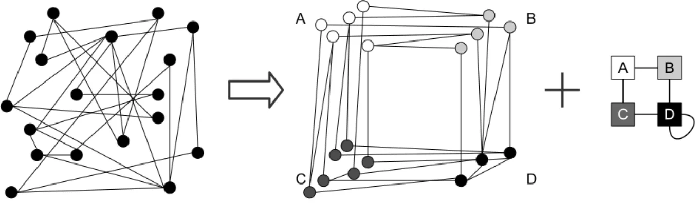
The structure of large networks is usually not comprehen-sible to the human beholder. Especially, if the network has not been designed by a human architect, but rather evolved over time in a complex (natural) process. Examples for such networks are social (friendship, mailing, scientific collaboration, advice giving), economic (trading between countries or companies), chemical (protein-protein reac-tions), biological (food chain), or internet link networks. Nevertheless, researchers in these fields use the networks to gain insight into their structural makeup. To this end, a first step is most often the reduction of the network’s complexity with the help of algorithms. A common ap-proach is to reduce the high number of nodes in the net-work. The idea ofblockmodeling approaches is to group the nodes such that the number of groups is much lower than the number of nodes. The grouping is done in a way that leads to patterns in the network’s links. We distinguish two kinds of patterns: Patterns of linkdensity(Section 1.1) and of link existence(Section 1.2). An example for pat-terns of link density is given in Figure 1: On the left-hand side, we see a random drawing of a graphG= (V, E). In the center, we see a partition ofV into four groupsA,B,
C,D, indicated by four different colors, such that a den-sity pattern becomes apparent. Densely connected are the group pairs AB, BD, DD, CD, CA, sparsely connected areAA, BB, CC, AD, BC. Note that we use a merely in-tuitive definition of density here for motivational reasons; strict mathematical definitions will be introduced subse-quently.
Before we explain the patterns of link density, we for-malize a vertex grouping of a graphGwith vertex setVand edge setEas a vertex coloring. This is possible since
ev-ery vertex coloringφ:V →[c], where[c] ={1,2, . . . , c}, naturally defines a partition of V into the color classes. W.l.o.g. we assume thatφis surjective, i.e., allccolors are used. In this paper, we assume that our network is given as an undirected graphG = (V, E). More general cases, in which there are weights (on the arcs or on group pairs) or multiple arc types are not treated here.
1.1
Patterns of link density
The goal of the grouping which is discussed in this section is to group the vertices in a way such that for each pair of groups, there are either verymanyor veryfewlinks be-tween the groups. In other words, we search for apattern of link densityin the network.
Once such a pattern has been found, the network’s com-plexity has been reduced in the following sense: One can now shrink the groups to single vertices, and connect two such vertices by an edge if the corresponding groups were densely connected prior to the shrinking. The shrunk graph for the example in Figure 1 is depicted on the right-hand side of the figure.
A
C
B
D
A B
C D
Figure 1:An exemplary density pattern.
figure. Note that the image graph can be seen as a simpli-fication of the network structure: There is an edge in the image graph wherever there are many edges in the original network, and no edge wherever there are only few edges.
For a given network graphG, one is hence interested in a coloringφof the vertices together with a density pattern. Such a pair(φ, I)of a coloringφand its interpretation, an image matrixIof appropriate dimension, is called a block-model. The process of computing a good blockmodel for a given network is sometimes calledblockmodeling.
1.2
Patterns of link existence
Density patterns imply that for the vertices in a groupA, it holds that either all of them have very many or all of them have very few links to the vertices in a groupB. In a pattern of linkexistence, however, one demands that either many vertices in groupAhaveat least onelink into groupB or almost no vertex in groupAhas a link to groupB. Analo-gously to the density pattern case, we can define an image matrix. It encodes for each pair of groups which of the two cases are interpreted to exist in the given coloring. The im-age graph then visualizes a pattern of connectivity. If an edge exists between groupsA and B, then almost every vertex inAis connected toB, and vice versa. Otherwise, the groups are almost disconnected.
1.3
Fixing patterns
To find a suitable number of groups is generally part of the blockmodeling process. In practical blockmodeling, how-ever, it is sometimes set a priori to a small fixed value. Moreover, the whole pattern is sometimes fixed a priori. The blockmodeling then reduces to the search for a color-ing which matches the given pattern best. This is useful to test whether an assumed pattern actually exists in the net-work. A prominent example of pattern fixing is the cluster-ing problem. Here, one searches for density patterns. The numbercof groups is fixed to a small value and the image matrix is fixed to thec×cidentity matrix. The blockmodel-ing hence consists of the search for a colorblockmodel-ing withccolors such that the color groups themselves are dense, whereas
their interconnections are sparse. In case thatcis not fixed, the family of all identity matrices is considered as the set of feasible patterns.
1.4
Outline of the paper
Literature shows a large variety in practical blockmodeling approaches. Not only are they distinct in the way they use a priori fixings, they also differ in the ways they measure the quality of a given blockmodel for a given network. Usu-ally, the search for clusters, link density and link existence patterns are treated separately. There are separate methods and publications for each of the three problem types.
In this paper, we present a new classification of the ap-proaches. This classification holds for all (non-stochastic) clustering and blockmodeling approaches which quantify the quality of blockmodels and are reported in the fol-lowing survey books: Social Network Analysisby Wasser-man and Faust [16],Network Analysisby Brandes and Er-lebach [6] (exceptconductance), andCommunity Detection in Graphsby Fortunato [10].
The search for an ideal blockmodel can usually be for-mulated as a graph coloring problem. By our classification, we show that the practical approaches can be seen as meth-ods to optimize very specific relaxations of these problems. They are the same in clustering, link density and link exis-tence patterns search.
Section 2 presents the graph coloring problems, which are relaxed in practical approaches. Section 3 explains the three types of relaxations that are used. Each type is il-lustrated with practical examples from the survey books. Finally, Section 4 summarizes and gives an outlook on ap-plications of the classification.
2
Ideal blockmodels
be directly constructed fromφ: The entryIAB is0if and only if there is no edge from A to B. We hence call a coloringφidealif the blockmodel(φ, I)is ideal, whereI
is constructed as explained.
There are three graph theoretical definitions of ideal col-orings. They will be presented in the next three subsec-tions.
2.1
The subgraph definition
In ideal blockmodels for density patterns, certain sub-graphs are either complete or empty. These subsub-graphs can be defined as follows. Given a coloringφ, there is one such subgraphGφ,A,B for every pair(A, B)of colors. It is ob-tained fromGby deleting all vertices but the ones colored withA or B and deleting all edges but those connecting an A-colored with a B-colored vertex. Gφ,A,B is hence bipartite forA 6=B. Note that all of these subgraphs are edge disjoint. A similar observation can be made for ideal link existence blockmodels: That all vertices inAhave at least one neighbor inB, and vice versa, is equivalent to the statement thatGφ,A,Bcontains no isolated vertices.
We have seen thatclusteringis a special case of link den-sity, where the image matrix is a priori fixed. However, there is a common variant of clustering. It only requires the color groups to be dense, but doesnotrequire their in-terconnections to be sparse. In other words, only the diag-onal image matrix entries are given. We include this vari-ant into our classification scheme as it is widely used. It corresponds to Part (i) of the following definition of ideal colorings. Part (ii) defines ideal link density and Part (iii) ideal link existence colorings. See Figure 2 for examples.
Definition 1. Given a graphG, ac-coloringφ:V →[c]
of its vertex set is
(i) anideal cliquec-coloring, if for allA∈[c], the graph
Gφ,A,Ais complete.
(ii) an ideal structural c-coloring, if for all color pairs
A, B ∈ [c], the graph Gφ,A,B is either empty or a
complete (complete bipartite forA6=B) graph.
(iii) an ideal regular c-coloring, if for all color pairs
A, B ∈[c], the graphGφ,A,B is either empty or
con-tains no isolated vertices.
2.2
The node pair definition
We have seen that ideal colorings can be defined by sub-graph characterizations. Alternatively, they can be de-fined by properties of same-colored vertices. In a clique
c-coloring, every two vertices with the same color are con-nected by an edge. In a structuralc-coloring, two vertices with the same color have exactly the same neighboring ver-tices in G. In a regularc-coloring, two vertices with the
to vertexu. The following definition is hence equivalent to the subgraph definition above. See Lorrain and White [12] for details.
Definition 2. Given a graphG, ac-coloringφ:V →[c]
of its vertex set is an
(i) ideal cliquec-coloring, if for allu, v∈V withφ(u) =
φ(v):uv∈E.
(ii) ideal structural c-coloring, if for allu, v ∈ V with
φ(u) =φ(v):N(u)\ {v}=N(v)\ {u}.
(iii) ideal regular c-coloring, if for all u, v ∈ V with
φ(u) =φ(v):{φ(w)| w∈V, uw ∈E} ={φ(w)|
w∈V, vw∈E}.
2.3
The single node definition
A definition from the perspective ofsinglevertex is only possible with respect to a fixed image matrix I. In this case, the following single node definition is equivalent to the two definitions above.
Definition 3. Given a graphGand ac×cimage matrixI, ac-coloringφ:V →[c]ofG’s vertex set is
(i) anideal cliquec-coloring, if for allu∈V:uis adja-cent to allv∈V withφ(v) =φ(u).
(ii) anideal structuralc-coloring w. r. t.I, if for allu∈V
and all C ∈ [c]: uis adjacent to all v ∈ V with
φ(v) =CifIφ(u)C= 1, and to nov∈V withφ(v) =
CifIφ(u)C= 0.
(iii) anideal regularc-coloring w. r. t.I, if for allu ∈V
and allC ∈[c]: uis adjacent to at least onev ∈V
withφ(v) =CifIφ(u)C = 1, and to nov ∈V with
φ(v) =CifIφ(u)C= 0.
3
Relaxations
For a given graphG, one can theoretically compute a col-oring from Definition 1 or 2 to obtain an ideal colcol-oring (and thus ideal blockmodel). However, this is usually not done in practice. In Section 3.1, we list some common rea-sons for this decision. In Section 3.2, we show that the ap-proaches used in practice can be interpreted as the solution of an optimization problem on a relaxed problem defini-tion.
3.1
Reasons for relaxations
There are several reasons for the use of relaxations instead of directly searching for ideal blockmodels. We list four of them.
a) b) c)
Figure 2:Ideal clique (a), structural (b), and regular (c)3-colorings. In b) and c), the corresponding image graph is depicted.
2. Real-world modeling reasons. The definition might be too restrictive for the application at hand. For ex-ample, the graph theoretical definition ofcliquemight be too strict to describe friendship cliques in social networks, where some edges can be missing.
3. Involvement of statistics.The relaxations allow to de-fine statistically profound criteria for the quality of colorings, instead of the purely graph theoretical ones.
4. Robustness against measuring errors. The extrac-tion of graphs from complex networks can be erro-neous, especially in biological or chemical networks. However, a regular coloring on a graph can turn non-regular by the deletion or addition of one single edge. Relaxations are hence useful to limit the influence of these errors on the colorings.
3.2
General relaxation
In this section, we show how ideal blockmodels are re-laxed in practice. Denote byCC(c, G)the set of all clique
c-colorings of the vertices of G. Analogously, we de-fine SC(c, G)andRC(c, G)for structural and regular c -colorings. As a shorthand, we simply write X(G) in a statement which holds for any fixed type (CC, SC, RC) and any fixed numbercof colors. Practitioners, often im-plicitly, enlarge the setX(G)of feasible colorings to a set
XL(G) ⊇ X(G)and assign a penalty valuep(φ) ≥0to each memberφ of the enlarged setXL(G). Afterwards, they solve the optimization problem of finding a color-ingφ∗inXL(G)with the minimum penalty valuep(φ∗). We now show that this is usually done in the following way: The setX(G)of feasible colorings is enlarged by dropping some of the requirements in the definition ofX. Further-more, the penalty functionpis not arbitrary, but measures the degree of violation against the droppedrequirements. The optimization problem to be solved is thus:
(MIN-P)Given the setXL(G)and the penalty function
p:XL(G)→R+0, find aφ∗∈XL(G)which minimizesp. That is, among the colorings satisfying the non-dropped requirements, find the one which violates the dropped re-quirements to the least possible extent. As a convention, a penalty value of0is assigned to the colorings inX(G), as
they do not violate any dropped requirements ( compatibil-ity requirement, see Doreian et. al. [9]). Hence, a coloring satisfying the original definitionX is always an optimum solution to (MIN-P).
We will now classify literature by the type of relaxation used. As we are considering the relaxation of ideal col-orings, three types of relaxations come to mind: The re-laxation of the coloring definition, of the node pair ideal-ity definition and the subgraph idealideal-ity definition. Indeed, these possibilities are widely used. In Section 3.3, we will look at the cases where the general definition of coloring is relaxed. Sections 3.4 and 3.5 treat the ideality definition relaxations respectively.
3.3
Coloring relaxations
In Definition 1 and 2 for ideal colorings, the definition of “coloring” itself can be relaxed. If we use the binary vari-ablesxvA to express whether vertex v is colored with A (xvA = 1) or not (xvA = 0), the requirement “to be a
c-coloring” can be decomposed into the following sub re-quirements:
c X
A=1
xvA= 1 for allv∈V, (1)
X
v∈V
xvA≥1 for allA∈[c], (2)
0≤xvA≤1 for allv∈V, A∈[c], (3)
xvA∈Z for allv∈V, A∈[c]. (4)
Example (Fuzzy Colorings.) In some applications, it is meaningful for a vertex to get several colors at the same time. E.g., a person might be a member of several clubs. In this case, requirement (1) is dropped. Alternatively, a vertex might be allowed to consist of color fractions that sum up to1, such as50%red,30%green and20%blue. In this case, requirement (4) is dropped. One speaks offuzzy coloringsorpartitionsin both of these cases of relaxation. Usually, there is no penalty for a vertex to have more than one color at the same time. That is, the penalty functionpis usually constant with respect to the coloring requirements.
bers are usually more suitable for interpretation, the penalty functionpmight be defined to assign each coloringφthe number of colors used byφ. The lower the number of col-ors, the less the amount of penalty. As an example, the algorithm CATREGE [4] solves (MIN-P) for such apand X=RC. I.e., given a graph, it finds a regularc-coloring with the smallest possiblec.
3.4
Single node and node pair relaxations
In single node relaxations, the properties for a single vertex to contribute to an ideal coloring are relaxed. As we have seen in Definition 3, single node definitions are only possi-ble if the image matrixIis fixed. An example are the nodal degree relaxations for clusterings, i.e., for Part (i).
Example (Nodal Degree Relaxations.)Seidman and Fos-ter [15] relax the requirement that every vertex must be adjacent to all other vertices of the same color by the re-quirement that every vertex can be non-adjacent to at most
kother vertices of the same color. In an ideal coloring, the resulting subgraphs are hence not cliques, but so-calledk -plexes. Usually, the relaxation is not penalized. That is,p
is constant, sayp≡0. The search for an ideal blockmodel is hence simply the search for a partition of the vertices intok-plexes. Instead ofk-plexes, the similark-cores are sometimes used.
We now turn to the more common nodepairrelaxations. Here, the properties for same-colored vertex pairs in Def-inition 2 are relaxed. Two forms ofpare most commonly used, which will be explained by the following two exam-ples: pis either constant or decomposable over the set of all vertex pairs.
Example (Sociometric Cliques.)Alba [1] finds the graph theoretical definition of cliqueto be not perfectly appro-priate to describe friendship (or sociometric) cliques in so-cial networks. He thus relaxes its definition to so-called
n-cliques. Here, two same-colored vertices do not need to be connected by an edge. They need to be connected by a path of length at most n, which relaxes the edge connec-tion requirement. If no penalties are introduced, the prob-lem (MIN-P) merely consists in the search foranypartition inton-cliques. Similar to then-clique are then-clan and
n-club relaxations [13].
We now treat a second common type of node pair relax-ation: Thevertex similarity approaches. The idea is to con-sider for each vertex pair separately, whether it should be same-colored or not. In this special case of (MIN-P), the penalty function pcan thus be decomposed over all ver-tex pairs, i.e., p(φ) = P
u,v∈V puvδ(φ(u), φ(v)). Here,
puv ≥ 0 are real numbers and δ denotes the Kronecker function. It is1ifφ(u) = φ(v)and0otherwise. In liter-ature, the numberspuvare often called(dis)similarity
val-ues. The relaxation technique of using such a decompos-able function is calledindirect blockmodeling approachby Doreian et al. [9].
propositions were made indirectly by a specification of the valuespuv. They quantify how much a coloring violates this dropped requirement, that is, to quantify how similar two vertices are with respect to common neighbors. See Leicht, Holme, and Newman [11] for an overview on these functions.
3.5
Subgraph relaxations
In subgraph relaxations, the requirements of Definition 1 for ideal blockmodels are relaxed.
Assume a practitioner is interested in regular4-colorings on a given graph G = (V, E). However, such a color-ing does not exist onG. It is then reasonable to consider a 4-coloring φ to be a good solution, if it is not regular on G, but turns regular ifG is changed by a very small amount. Following this idea, the best4-coloring is the one that requires the lowest amount of changes inGin order to become regular. Possible changes are usually the deletion and addition of edges. That is, requirements of the forms “uv∈E” and “uv /∈E” are dropped. If they are penalized by the functionp, then the coloringφ∗which requires the lowest amount of edge changes in Gwill be the optimal solution to (MIN-P).
In order to define a suitable penalty functionp, we first need to define a functiondto measure the amount of edge changes. More precisely,dmeasures the distance of two graphsG = (V, E)andH = (V, F)on the same vertex setV. A simple but common exemplary form of such ad
is given by
d(G, H) = X u,v∈V,u6=v
|A(G)u,v−A(H)u,v|, (5)
whereAdenotes the adjacency matrix of the graph. The function counts the number of different entries in the adja-cency matrices ofGandH. More complex distance func-tions are discussed below. The functiondmeasures the dis-tance ofGto a single graphH. We can also measure its dis-tance to a set of graphsH, by defining the distanced(G,H) as the distance ofGto its closest element inH. That is,
d(G,H) := min H∈H
d(G, H).
To measure how muchGhas to be changed, it is compared to sets of ideal graphsH(φ), on whichφperfectly satisfies the requirements. In our example, H(φ) is defined such thatφis4-regular on allH ∈ H(φ). The penalty function for (MIN-P) is hencep(φ) =d(G,H(φ)).
Ideal, Worst and Average Graphs
Given an ideal coloring definition X (for example CC, SC, RC), a graphG= (V, E)and a coloringφof its vertices, the set H(φ)of ideal graphs can be naturally defined. It is the set of all graphs H with the same vertex set asG, such that φis an X-coloring on H. Definition 1 gives a characterization of these graphs. In the case of clustering, i. e., X = CC, the ideal graphs are those in which vertices of the same color induce complete graphs. Note that for everyφ:V →[c], the setH(φ)is non-empty.
Alternatively, one can defineH(φ)to be the set ofworst
graphs instead of ideal ones. Worst graphs can be easily defined for CC and SC. This is because their subgraph char-acterization in Definition 1 use empty and complete graphs only. As “being empty” and “being complete” are opposite extremes, one can define worst graphs by interchanging the words “empty” and “complete” in the definition. E. g., in a worst graph for clustering (CC) no cluster contains any edges. If worst graphs are used, the distance of the closest graph toGneeds to be maximized instead of minimized. A third alternative has been used for CC and SC: G is compared to average graphs. For clustering, the subgraphs are hence neither empty nor complete, but have an average density. The distance ofGto the average graphsH(φ)can then be positive or negative, depending on whether Gis worse (sparser) or better (denser) than average. The same holds hence for the penalty function. It is usually used as a reward functionp: The fartherGis from average in the positive direction, the largerpis, and the betterφis.
Overview on Distance Functions
We already stated the most simple distance function to measure the distance between two graphs on the same ver-tex set:
d(G, H) = X
u,v∈V,u6=v
|A(G)u,v−A(H)u,v|,
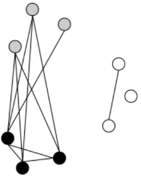
It counts the number of edges to be added or deleted (changed) inGto obtain the ideal graphH. See Figure 3 for an example for structural 3-colorings (X = SC). The dis-tanced(G,H(φ))of the depicted coloringφof the drawn graphGis3. The reason is that3changes are at least neces-sary to obtain a structural3-coloring: Add two edges from gray to black and delete one edge within white. Hence, the penalty value for this coloring isp(φ) = 3.
IfGis compared toaveragegraphs, the absolute value function is a problem. Here, we want to distinguish whetherGis worse or better than average. Hence, the fol-lowing function is more suitable in this case.
d(G, H) = X u,v∈V,u6=v
(A(G)u,v−A(H)u,v). (6)
The adjacency matrix ofHis possibly weighted, as average graphs usually do not have binary edge weights.
There is a third function for the case that vertices are relaxed instead of edges. More precisely, if requirements
Figure 3:Example for the distance function (5) when applied to a structural 3-coloring problem.
of the form “v ∈ V” are relaxed. Note that the opposite requirement “v /∈ V” is never relaxed, as the addition of vertices cannot contribute to the transformation ofGinto an ideal graph. For every coloringφof the vertices inG= (V, E),Gis compared to a set of ideal graphsH(φ). Ev-ery such graphH = (VH, EH)inH(φ)has a vertex sub-setVH ⊆V and the edge setEH = E(VH). That is,H can be obtained fromGby deleting vertices together with their incident edges. A distance function needs to measure the amount of vertices to be deleted to transformGintoH.
d(G, H) =|V(G)| − |V(H)|. (7)
Beside these linear functions, several non-polynomial functions have been proposed. Being derived from general statistical matrix correlation measures, they can be used to compare the adjacency matrices ofGandH. See Wasser-man and Faust [16] or Arabie et al. [2] for an overview.
Combining Subgraph Penalties
In Definition 1, the ideal coloring conditions are formu-lated as requirements for the subgraphs Gφ,A,B ofG. In the widely useddirect blockmodeling approach, these sub-graphs are relaxed separately. That is, there is a separate penalty value for each subgraph. However, the same dis-tance functiondis used for each subgraph. Whether the separate relaxations of the subgraphs is equivalent to the relaxation ofGitself depends on the choice ofd. In direct blockmodeling, we have single penalty valuespAB(φ) =
d(Gφ,A,B,Hφ,A,B) for the subgraphs. They need to be combined to a total penalty valuep(φ). In most cases, the
pABare simply summed up:
p(φ) = X
A,B∈[c]
pAB(φ). (8)
For clustering (X=CC), the sum runs clearly only over those(A, B)withA = B. If scaling is used, the factor is usually1/mAB, wheremAB is the number of possible edges in the subgraph Gφ,A,B. More precisely, mAB = |A| · |B|ifA6=B,mAA=|A| ·(|A| −1), and
p(φ) = X
A,B∈[c]
1
mAB ·
approaches.
p(φ) = X
A,B∈[c]
(pAB(φ))2. (10)
Besides the above scaling factor, a second one can be used here. The distance ofGφ,A,B to Hφ,A,B can be seen in relation to the maximum distancedmaxφ,A,B of any graph, on the same vertex set, toHφ,A,B.
p(φ) = X
A,B∈[c] mAB·
pAB(φ)
dmaxφ,A,B
2
. (11)
Examples
We now give some examples on how this kind of relaxation is used in literature, either for coloring type CC, SC, or RC. For each example, we need to specify the following modeling choices:
– Whether ideal, worst, or average graphs are used (and how average is defined).
– Whether edges or vertices are relaxed.
– Howp(φ)is combined from thepAB(φ).
Example (Cluster Performance). Theperformanceof a clustering counts the number of missing edges within the clusters and adds the number of existing edges between the clusters. It is hence a measure for the clustering special case ofX = SC. According to our classification, ideal graphs are used, edges are relaxed, andp(φ)is simply the sum of thepAB(φ).
Example (Maximal Cluster Density.) A basic measure for the quality of a clustering (X=CC) onG= (V, E)is the sum over allintra-cluster densitiesδint(Vi). They give the proportion of actual edges to theoretically possible edges within thei-th cluster:
δint(Vi) =
# internal edges ofVi |Vi|(|Vi| −1)/2
.
The search for a coloring φ∗ with maximum total intra-cluster density is a (MIN-P) problem. Ideal graphs are used, edges are relaxed, and the penalty valuespAB(φ)are linearly combined by Formula (9).
Example (Maximal Structural Density.) Wasserman and Faust explain a simple measure for structural colorings in their survey [16]. It is a generalization of the preced-ing example from clique to structural colorpreced-ings. For each pairA, Bof colors, they sum up the values|IAB−∆AB|. Here, I denotes the image matrix and ∆AB denotes the density. The density is defined as the number of edges from
A-colored toB-colored vertices, divided by the maximum possible numbermAB of such edges. Hence, ideal graphs are used, edges are relaxed, and the penaltiespAB(φ)are linearly combined by formula (9).
They chooseH(φ)to contain average graphs. More pre-cisely, H(φ)consists of exactly one graphH = (V, F). The edge weight ofuv ∈ F isdeg(u)deg(v)/2|E|. This is precisely the probability of the edge to exist in a ran-dom graph with the same degree distribution asG. For this reason,H can be interpreted as the average graph w.r.t. to the degree distribution of G. Hence, average graphs are used, edges are relaxed, and the penaltiespAB(φ)are sim-ply summed up (Formula (8)).
Note thatp(φ)/2|E|is called themodularityofφ. The factor1/2|E|is however constant and can thus be ignored in the solution of (MIN-P). Other so-called Newman-like modularitiescan be modeled analogously.
Example (Berkowitz-Carrington-Heil Index.) The in-dex [8] is designed for structural colorings (X=SC). It com-paresGto an average graphH. The user is asked to spec-ify an average densityαfrom the interval between0and1.
H is then the complete graph with edge weights allα, let-ting its density equal α. The distance function d is (5), hence the most simple one. It is applied on subgraphs. Since the index is aχ2approach, the functionp(φ)is
com-posed as in (11).
Example (Vertex Relaxation.) Batagelj et. al. [3] re-lax vertices for regular colorings (X=RE). They use ideal graphs, relax vertices, and simply sum up the penal-tiespAB(φ). However, they restrict the natural setH(φ)of ideal graphs by allowing only thoseH ∈ H(φ)for which it holds that whenever there is an edgeuv ∈ E anduis not inVH, thenvcannot be inVH either. An optimization heuristic for this function is implemented in UCINET [5]. Brusco and Steinley [7] present an exact optimization algo-rithm based on an integer programming model.
4
Summary and conclusions
We present a classification for clustering and blockmodel-ing approaches used in practice. We show that these ap-proaches are based on relaxations of graph theoretical col-oring definitions. Basically, there are only three types of re-laxations. The classification unifies link density pattern (in-cluding clustering) and link existence pattern approaches and shows the connections between them.
An obvious drawback of such a theory about used ap-proaches is clearly its invalidity as soon as new kinds of approaches are invented. Furthermore, it does not yet cover approaches which penalize blockmodels in which the col-ors groups do not have similar sizes. An example is the
include it as most approaches deal with this requirement in-directly: They exclude blockmodels with largely differing group sizes from the setXL(G)of feasible blockmodels.
However, we also see two kinds of practical benefits. First, the classification can be used to think about the “missing” approaches. For example, approaches which use average graphs usually compare G to a single aver-age graph H, whose edge weights are fractional. This choice seems to be arbitrary, as one could also use a whole setH(φ)of unweighted average graphs for the comparison toG. The latter idea is standard if ideal instead of aver-age graphs are used. Second, the question which approach is the most suitable one for a given network can now be answered stepwise: Are ideal or average graphs more suit-able, should edges or vertices be relaxed, should node pairs or subgraphs be relaxed, how should subgraph penalties be combined, etc.?
References
[1] R. D. Alba. A graph-theoretic definition of a socio-metric clique. Journal of Mathematical Sociology, 3(1):113–126, 1973.
[2] P. Arabie, S. A. Boorman, and P. R. Levitt. Construct-ing blockmodels: How and why. Journal of Mathe-matical Psychology, 17(1):21–63, 1978.
[3] V. Batagelj, P. Doreian, and A. Ferligoj. An optimiza-tional approach to regular equivalence. Social Net-works, 14(1):121–135, 1992.
[4] S. P. Borgatti and M. G. Everett. Two algorithms for computing regular equivalence. Social Networks, 15(4):361–376, 1993.
[5] S. P. Borgatti, M. G. Everett, and L. C. Freeman. Ucinet for windows: Software for social network analysis. 2002.
[6] U. Brandes and J. Lerner. Structural similarity: spec-tral methods for relaxed blockmodeling. Journal of Classification, 27(3):279–306, 2010.
[7] M. J. Brusco and D. Steinley. Integer programs for one-and two-mode blockmodeling based on pre-specified image matrices for structural and regular equivalence. Journal of Mathematical Psychology, 53(6):577–585, 2009.
[8] P. J. Carrington, G. H. Heil, and S. D. Berkowitz. A goodness-of-fit index for blockmodels. Social Net-works, 2(3):219–234, 1980.
[9] P. Doreian, V. Batagelj, and A. Ferligoj. General-ized blockmodeling, volume 25. Cambridge Univer-sity Press, 2005.
[10] S. Fortunato. Community detection in graphs.
Physics Reports, 486(3):75–174, 2009.
[11] E. Leicht, P. Holme, and M. Newman. Vertex simi-larity in networks.Physical Review E, 73(2):026120, 2006.
[12] F. Lorrain and H. C. White. Structural equivalence of individuals in social networks. The Journal of Math-ematical Sociology, 1(1):49–80, 1971.
[13] R. J. Mokken. Cliques, clubs and clans. Quality and Quantity, 13:161–173, 1979.
[14] M. E. Newman and M. Girvan. Finding and evalu-ating community structure in networks. Physical Re-view E, 69(2):026113, 2004.
[15] S. Seidman and B. Foster. A graph-theoretic general-ization of the clique concept. Journal of Mathemati-cal Sociology, 6:139–154, 1978.