Differential Evolution Control Parameters Study for Self-Adaptive Triangular
Brushstrokes
Aleš Zamuda and Uroš Mlakar
Faculty of Electrical Engineering and Computer Science, University of Maribor Smetanova ulica 17, SI-2000 Maribor, Slovenia
E-mail: [email protected], [email protected]
Keywords:differential evolution, evolutionary computer vision, evolutionary art, image-based modeling, self-adaptation, triangular brushstrokes
Received:December 1, 2014
This paper proposes a lossy image representation where a reference image is approximated by an evolved image, constituted of variable number of triangular brushstrokes. The parameters of each triangle brush are evolved using differential evolution, which self-adapts the triangles to the reference image, and also self-adapts some of the control parameters of the optimization algorithm, including the number of trian-gles. Experimental results show the viability of the proposed encoding and optimization results on a few sample reference images. The results of the self-adapting control parameters for crossover and mutation in differential evolution are also compared to results with keeping these parameters constant, like in a basic differential evolution algorithm. Statistical tests are furthermore included to confirm the improved perfor-mance with the self-adaptation of the control parameters over the fixed control parameters.
Povzetek: V ˇclanku je predlagana izgubna predstavitev slike, kjer je referenˇcna slika aproksimirana z evoluirano sliko, ki je sestavljena iz spremenljivega števila potez trikotniškega ˇcopiˇca. Parametre vsake poteze ˇcopiˇca optimiramo s pomoˇcjo diferencialne evolucije, ki samoprilagaja trikotniške poteze na ref-erenˇcno sliko in prav tako samoprilagaja nekatere krmilne parametre samega optimizacijskega algoritma, vkljuˇcno s številom trikotnikov. Rezultati poizkusov kažejo primernost predlagane metode in rezultati op-timizacije so prikazani za veˇc izbranih referenˇcnih slik. Rezultati samoprilagodljivih krmilnih parametrov za diferecialno evolucijo so primerjani tudi z rezultati, kjer so ti parametri nespremenljivi, kot je to primer pri osnovnem algoritmu diferencialne evolucije. Dodatno so podani še statistiˇcni testi, ki nadalje potrju-jejo izboljšanje kakovosti pristopa ob samoprilagajanju krmilnih parametrov v primerjavi s pristopom z nespremenljivimi krmilnimi parametri.
1
Introduction
In this paper, evolvable lossy image representation utiliz-ing an image compared to its evolved generated counterpart image, is proposed. The image is represented using a vari-able number of triangular brushstrokes [7], each consist-ing of triangle vertices coordinates and color parameters. These parameters for each triangle brush are evolved using differential evolution [13, 4], which self-adapts the control parameters, including the proposed self-adaptation for the number of triangles to be used. Experimental results show the viability of the proposed encoding and evolution con-vergence for lossy compression of sample images. Since this paper is an extended version of [8], new additional re-sults are included, where the experiments rere-sults with fixed control parameters for differential evolution are included to check and demonstrate the self-adaptation mechanism influence on results. The results show clear superiority of the proposed approach with the self-adaptive control pa-rameters over the approach where its control papa-rameters are fixed.
The approach presented is built upon and compared
In the following section, related work is presented, then the proposed approach is defined. In Section 4, the experi-mental results are reported. Section 5 concludes the paper with propositions for future work.
2
Related Work
In this section, related work on evolutionary computer vi-sion, evolutionary art, image representation, and evolution-ary optimization using differential evolution, are presented. These topics are used in the proposed method, defined in the next section.
2.1
Image-Based Modeling, Evolutionary
Computer Vision, and Evolutionary Art
Image-based approaches to modeling include processing of images, e.g., two-dimensional, from which after segmenta-tion certain features are extracted and used to represent a geometrical model [10]. For art drawings modeling, au-tomatic evolutionary rendering has been applied [2, 12]. Heijer and Eiben evolved pop art two-dimensional scal-able vector graphics (SVG) images [6] and defined genetic operators on SVG to evolve representational images using SVG, and also to evolve new images, different from source images, leading to new and surprising images for pop-art. Bergen and Ross [3] interactively evolved vector graph-ics images using genetic algorithm, where solid-coloured opaque or translucent geometric objects or mosaic tile ef-fects with bitmap textures were utilized; they considered the art aspect of the evolved image and multiple possible outcomes due to evolution stochastics and concluded to in-vestigate vector animation of the vectorized image.
In [14] animated artwork is evolved using an evolu-tionary algorithm. Then, Izadi et al. [7] evolved trian-gular brushstrokes challenge using genetic programming for two-dimensional images, using unguided and guided searches on a three or four branch genetic program, where roughly 5% similarity with reference images was obtained on average per pixel. In this paper, we build upon and com-pare our new approach with [7], by addressing and also ex-tending this challenge. After exex-tending the challenge, we optimize it using DE, which is described in the next sec-tion.
2.2
Evolutionary Optimization Using
Differential Evolution
Differential evolution (DE) [13] is a floating-point encod-ing evolutionary algorithm for continuous global optimiza-tion. It has been modified and extended several times with various versions being proposed [5]. DE has also been ap-plied to remote sensing image subpixel mapping [18], im-age thresholding [11], and for imim-age-based modeling using evolutionary computer vision to reconstruct a spatial pro-cedural tree model from a limited set of two dimensional
images [16, 15]. DE mechanisms were also compared to other algorithms in several studies [17]. Neri and Tirronen in their survey on DE [9] concluded that, compared to the other algorithms, a DE extension called jDE [4], is supe-rior to the compared algorithms in terms of robustness and versatility over a diverse benchmark set used in the survey. Therefore, we choose to apply jDE in this approach.
The original DE has a main evolutionary loop where a population of vectors is computed within each genera-tion. For one generation, counted as g, each vector xi,
∀i ∈ {1, . . . ,NP}in the current population of size NP, undergoes DE evolutionary operators, namely the muta-tion, crossover, and selection. Using these operators, a trial vector (offspring) is produced and the vector with the best fitness value is selected for the next generation. For each corresponding population vector, mutation creates a mutant vectorvi,g+1(‘rand/1’[13]):
vi,g+1=xr1,g+F(xr2,g−xr3,g), (1)
where the indexes r1, r2, and r3 are random and mutu-ally different integers generated in from set{1, . . . ,NP}, which are also different fromi. F is an amplification fac-tor of the difference vecfac-tor, mostly within the interval[0,1]. The termxr2,g−xr3,gdenotes a difference vector, which is
named the amplified difference vector after multiplication withF. The mutant vectorvi,g+1is then used for
recom-bination, where with the target vector xi,g a trial vector
ui,j,g+1is created, e.g., using binary crossover:
ui,j,g+1=
vi,j,g+1, ifrand(0,1)≤CR
orj=jrand,
xi,j,g otherwise,
(2)
where CR denotes the crossover rate, ∀j ∈ {1, . . . , D}
is aj-th search parameter ofD-dimensional search space,
rand(0,1)∈[0,1]is a uniformly distributed random num-ber, andjrand is a uniform randomly chosen index of the
search parameter, which is always exchanged to prevent cloning of target vectors. The original DE [13] keeps the control parameters fixed, such asF = 0.5andCR = 0.9
throughout optimization.
However, the jDE algorithm, which is a modification of the original DE, self-adapts theFandCRcontrol parame-ters to generate the vectorsvi,g+1andui,g+1,
correspond-ing values Fi andCRi, ∀i ∈ {1, . . . ,NP} are updated
prior to their use in the mutation and crossover mecha-nisms:
Fi,g+1= (
Fl+rand1×Fu ifrand2< τ1,
Fi,g otherwise,
(3)
CRi,g+1= (
rand3 ifrand4< τ2,
CRi,g otherwise,
(4)
vector and propagates the fittest:
xi,g+1= (
ui,g+1 iff(ui,g+1)< f(xi,g),
xi,g otherwise.
(5)
3
Differential Evolution for
Self-Adaptive Triangular
Brushstrokes
In this section, the encoding aspect, genotype-phenotpye rendering, and evaluation mechanisms of the proposed ap-proach are defined.
3.1
Encoding Aspect
We encode an individual compressed image into a DE vector as follows. A DE vector
x = (x1, x2, . . . , x8Tmax, Fi,CRi, TiL, TiU) is
com-posed of floating-point scalar values packed sequentially as{xj : ∀j ∈ {1, . . . , D+ 4}}, starting with a
triangles-coding part of length D = 8Tmax, and the rest are the self-adaptive control parameters of the vector to be used during the DE. The self-adaptive control parameters part of thexvector encodes and uses the scaling factorF and crossover rate CR as in the jDE [4]; then the TL
i , TiU
∈ {1, . . . , Tmax}control parameters follow.
The self-adaptiveTL
i andTiUcontrol parameters
deter-mine index-wise triangles encoded in the vector xto be used for rendering the evolved image, i.e., the portion ofx
to render an image is{xj :∀j ∈ {TiL, . . . , TiU}}.
In this paper, we propose to have the whole vector rep-resent a triangle set, organized similar to serializing a tree as a linear vector in visiting nodes by depth-first search. However, the leaf nodes are mostly exposed to being cut-off, whereas the root node is encoded in the middle of the vector and the near-root nodes are therefore more protected in being retained, since they are more anchored due to cut-offs mostly around the codon edges. After being included into a new trial vector, all nodes have an equal probability of having their triangle data changed.
In this way, theTL
i andTiU allow us to render only a
sub-portion of the triangles set, similarly to taking an in-separable portion of a GP tree traversal as in [7]. This gives us an arbitrary length render set, and keeps the crossover of anti-codon to help us find the number of triangles Ti ∈
{1, . . . , Tmax}, which is more suitable for image
approxi-mation:
Ti=
( TU
i −TiL+ 1 ifTiL< TiU
(Tmax−TL
i ) +TiU otherwise.
(6)
TheTL
i andTiUare updated similarly to theFicontrol
pa-rameter:
Ti,gL+1= (
brandL
1×Tmaxc ifrandL2< τL,
Ti,gL otherwise, (7)
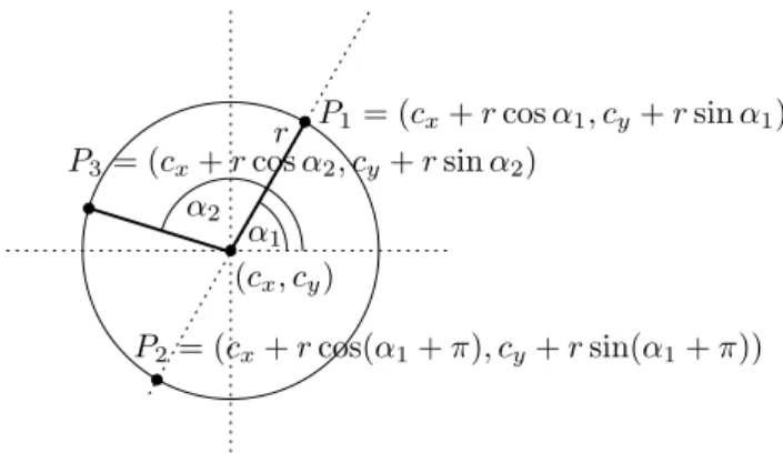
Figure 1: The triangle brush definition and the circum-scribed circle.
Ti,gU+1= (
brandU
1 ×Tmaxc ifrandU2 < τU, TU
i,g otherwise,
(8)
whereτL=τU=τ
1= 0.1of the jDE.
3.2
Genotype-Phenotype Rendering
A DE vectorxi,∀i∈ {1, . . . ,NP}encoded using
floating-point numbers xi,j,∀j ∈ {1, . . . , D+ 4} constituting a
genotype is rendered into a phenotype imagezi={zi,x,y}
of Rx width and Ry height in pixels, to be compared against a reference imagez∗as follows.
The triangle brushstrokes (Figure 1) are represented as
(cx, cy, r, α1, α2, bY, bCb, bCr), where cx ∈ [0, . . . , Rx), cy ∈ [0, . . . , Ry), andr ∈ [0, Rx/
√
Tmax] define the
cir-cumscribed circle center and radius for the triangle to be rendered; α1 ∈ [1◦,360◦)andα2 ∈ [1◦,180◦)define the vertices of this triangle on its circumscribed circle; and
bY∈[16,236),bCb∈[16,241), andbCr ∈[16,241)are the
color components of the brush for the triangle contained pixels.
The triangles’ vertices coordinates encoded by i-th DE vector construct Ti triangles, each triangle Tk =
(cx,k, cy,k, rk, α1,k, α2,k),∀k ∈ {1, . . . , Ti} (Tk being
packed asxi = {xi,j}, j = 8k+m,m ∈ {1, . . . ,8}),
defining the vertices of a triangleP1,k,P2,k, andP3,k:
P1,k=b(cx,k+rkcosα1,k,
cy,k+rksinα1,k)c,
(9)
P2,k=b(cx,k+rkcos(α1,k+π),
cy,k+rksin(α1,k+π))c,
(10)
P3,k=b(cx,k+rkcosα2,k,
cy,k+rksinα2,k)c.
(11)
The brush color bYCbCr
k = (b
Y
k, b
Cb
k , b
Cr
k) is first
trans-formed into RGB color model as bRGB
k = (b
R
k, bGk, b
B
k)
(bR
k, bGk, bBk ∈[0,255]), where:
bRk =
1.164(bYk−16) + 1.596(bCrk −128)
bG
k =b1.164(bYk −16)−0.813(bCrk −128)
−0.391(bCbk −128)c (13)
bBk =
1.164(bYk−16) + 2.018(bCbk −128)
(14)
For each triangle Tk, a solid color is rendered without
antialiasing over the triangle brush area rasterizing [1] with a transparency factor of1/Ti:
bk=
255
Ti
bRGBk
. (15)
This is analogous to blending the triangle as a part-transparent layer within the evolved imageZi=Pkzk,x,y
and computes R, G, and B color layers for the pixels of the
i-th individual:
zk,x,y=
X
Tkover (x,y)
bk,x,y
= X
Tkover (x,y)
255
Ti
bRGBk,x,y
,
(16)
whereTkover (x, y)denotes each triangle being rendered
over the pixel(x, y)such thatbk,x,ycontains the rendered
pixels of a brushstroke. Triangles defined possibly over the edges of image canvas are drawn by clipping away pixels outside of the canvas area.
The initialization of a genotype is such that the
cx, cy, α1, α2, bY, bCb,bCr,TiL, andTiUare initialized
uni-form randomly to integer values within their respective def-inition intervals, whileris kept as a floating-point. All pa-rameters are however evolved as floating-point scalar val-ues in DE.
3.3
Evaluation
Evaluation of the phenotype image Zi to be compared
against a reference image Z∗ is as follows. A reference image Z∗ is represented as RGB-encoded colored pixels integer values in layersZ∗={(zR
x,y, zGx,y, zx,yB )}.
To obtain a difference assessment value, the following comparison metric is used for comparing an evolved image Z=ZitoZ∗:
f(Z) = 100×
Ry−1
X
y=0
Rx−1
X
x=0
|z∗x,yR−zRx,y|
255×RxRy
+
Ry−1
X
y=0
Rx−1
X
x=0
|zx,y∗G−zx,yG |
255×RxRy +
Ry−1
X
y=0
Rx−1
X
x=0
|z∗x,yB −zx,yB |
255×RxRy
. (17) 5 10 15 20 25 30 35 40
0 500 1000 1500 2000
Fitness Generation Liberty Palace Vegetables Baboon
Figure 2: Fitness convergence, for best runs of each test image.
4
Experiments
The following experiments assess the viability of the ap-proach on different control parameters, each with several independent runs. The parameter sets are as follows: the DE population size NP = {25,50,100} and Tmax = {10,20, . . . ,150}, thereby for each run RNi={0, 1, . . . , 51} this counts for total of 45 parameter sets, i.e., 2340 independent runs. The NP and Tmax are fixed during
one run. The maximum number of function evaluations (MAXFES) used is same as with [7], MAXFES is105. For
image rendering, basic GDI+ is used.
4.1
Obtained Results
The obtained fitness values at the MAXFES termination of
105, over different parameters ofT
max andNP, are seen
in Tables 1 and 2. The best values obtained overall for an image are marked in bold underlined text font. The fitness convergence graphs for these best runs are seen in Figure 2, where after the initialization, the fitness is roughly below 40 (i.e., 40% similarity with reference), then drops below 15 for all test images and even further to slightly above 6 for two of them.
The convergent obtained results depend on the MAXFES used being same as with [7], but also NP and
Tmax, as reported below. From Tables 1 and 2, we choose to
report further evolved images up to MAXFES of106with
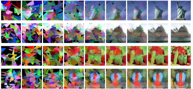
all images. The best approximated images after MAXFES of 106 are shown in the Figure 3 which shows the
evo-lution of the four images. In each line of Figure 3, the best fitting vectors upto MAXFES of 106 in generations g={0,100,200,400,700,1200,2000}, and the final gen-eration, are shown, then the rightmost the corresponding reference image. Figure 4 shows for each test image, dy-namics of the number of triangle brushes in current best vector during generations, displaying varying convergent bestTivalues across images.
Figure 3: The evolved and the reference images (self-adaptiveFandCR).
also makes ourNP parameter have higher value, since we have no guided search and the problem is therefore more general. Also, our approach does not use a dynamically re-allocatable morphable variable-size tree structure as in ge-netic programming encoding, inspite it rather uses a fixed size vector and limits its brushstrokes set by two simple bounds, making the approach faster for execution.
For comparison purposes and since this paper is an ex-tended version of [8], following additional comparison is included. The algorithm is run again with fixed control pa-rametersF = 0.5andCR = 0.9in DE, all other settings are kept same as with the proposed above approach.
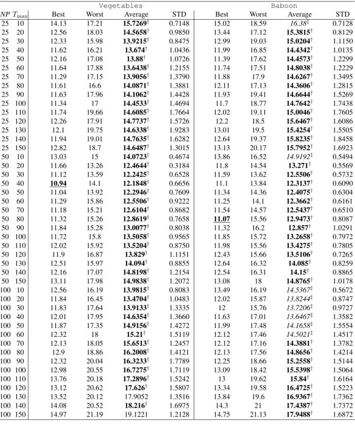
Further, the results in Tables 1 and 2 are statistically tested using t-test with alpha = 0.001, against the null hypothesis, that the results obtained with fixed control pa-rameters F = 0.5 and CR = 0.9 in DE, do not statis-tically differ. The symbol † with the values in bold text font signifies that the self-adaptive F andCRparameters approach results are significantly better and the symbol ‡ with values in italicized text font signifies that the fixed parameters approach results are significantly better. Com-paring the statistics on the varied N P andTmax settings,
DE with changingFandCRis 164 times better, 13 times worse, and 3 times with no significant performance differ-ence, compared to the DE withF = 0.5,CR= 0.9.
The Figure 5, the best DE run withF = 0.5,CR= 0.9, nonetheless still shows self-adaptation of the Ti
parame-ter – this is an additional indicator that the performance difference lines in the changing of theF andCRcontrol parameters, which, compared to fixed values, improve the approach performance if they are self-adaptive.
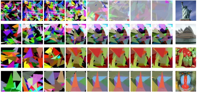
Visually, the performance difference is observed from the rendered images in Figure 6, showing superiority of the proposed approach with self-adaptive control parame-ters over the approach using fixed control parameparame-ters. The Figure 7 shows fitness convergence of the best evaluated vector of the best DE run withF = 0.5,CR = 0.9, this
10 20 30 40 50 60 70 80
0 500 1000 1500 2000
Ti
Generation
Liberty Palace Vegetables Baboon
Figure 4: Number of brushstrokes in best vector, for best runs of each test image, self-adaptiveF andCR parame-ters.
0 5 10 15 20 25 30
0 200 400 600 800 1000
Ti
Generation
Liberty Palace Vegetables Baboon
Table 1: Obtained fitness overTmaxandN P: test instancesLibertyandPalace
Liberty Palace
NPTmax Best Worst Average STD Best Worst Average STD
25 10 8.29 11.99 9.93096† 0.8233 8.69 13.69 10.1362† 0.9655
25 20 8.03 13.14 10.0935† 1.0845 7.83 11.5 9.12173† 0.8092
25 30 8.41 13.74 10.0525† 1.1712 7.52 11.1 8.97942† 0.7992
25 40 8.13 12.81 10.4408† 1.1416 7.34 11.36 8.91788† 0.8922
25 50 8.49 13.37 10.6767† 1.1768 7.65 12.53 8.87442† 0.9788
25 60 7.95 14.65 10.9858† 1.4284 7.9 11.88 8.99673† 0.8761
25 70 8.28 14.21 11.4075† 1.3630 7.79 13.17 9.50327† 1.0482
25 80 8.72 15.89 11.7554† 1.6330 7.97 12.34 9.43558† 0.9765
25 90 8.84 16.24 12.1342† 1.6608 8.41 13.54 9.82† 1.2756
25 100 9.01 16.74 12.4798† 1.7521 8.62 12.96 9.83635† 0.8869
25 110 8.07 16.78 12.7412† 1.7849 9.01 14.42 10.4119† 1.2468
25 120 9.67 16.14 12.8467† 1.7359 8.93 15.13 10.3858† 1.3149
25 130 10.16 17.96 13.2692† 1.7193 9.02 14.2 10.2858† 1.0292
25 140 9.29 17.99 13.7029† 1.7886 8.29 13.51 10.7779† 1.0299
25 150 10.82 18.56 14.0373† 1.6573 9.89 14.91 11.1206† 1.0586
50 10 7.51 9.69 8.45077† 0.4198 7.43 11.84 8.68058† 0.8825
50 20 6.78 8.99 7.80173† 0.4987 7.1 11.39 8.79173† 0.9592
50 30 6.89 9.17 7.81788† 0.5119 7.53 12.58 9.75654† 1.1186
50 40 6.77 9.87 8.0375† 0.6578 8.27 12.24 10.0575† 0.9537
50 50 7.08 10.61 8.39923† 0.7056 7.97 13.14 10.3338† 1.1009
50 60 7.15 10.4 8.67115† 0.7472 8.59 12.49 10.7817† 1.0754
50 70 7.46 10.9 9.1025† 0.8666 7.58 12.8 10.7744† 1.1086
50 80 7.6 11.4 9.47981† 0.8689 9.15 13.11 11.3802† 1.0178
50 90 8.05 12.65 9.67346† 0.9115 9.97 13.41 11.5227† 0.9315
50 100 8.75 11.75 10.0152† 0.7824 8.55 13.62 11.4356† 0.9923
50 110 8.93 13.63 10.6356† 0.9682 9.32 13.77 12.0712† 0.9579
50 120 9.22 13.01 10.7502† 0.9840 9.77 14.21 12.429† 0.8972
50 130 9.42 12.59 11.0527† 0.7707 11.37 14.07 12.7387† 0.6134
50 140 9.99 13.39 11.5719† 0.7815 9.69 15.5 12.9317† 0.9708
50 150 10.2 14.56 12.2633† 1.0702 9.58 15.36 12.8092† 1.1717
100 10 7.1 9.12 7.98596† 0.4241 7.91 13.88 10.9573† 1.8019
100 20 6.85 9.77 7.83962† 0.5360 8.86 14.59 12.1117† 1.2862
100 30 7.15 11.8 8.49077† 1.1563 9.59 16.15 12.9098† 1.0589
100 40 7.22 13 8.86327† 1.1092 9.65 14.97 13.2477† 1.1543
100 50 7.41 12.75 9.34846† 1.3939 11.01 15.52 13.8606† 0.9750
100 60 8.06 12.97 9.77731† 1.1539 11.5 16.14 14.1856† 1.1234
100 70 8.67 13.28 10.1954† 1.3722 10.77 16.32 14.3629† 1.1713
100 80 8.73 14.48 11.0929† 1.4093 10.98 17.06 14.9348† 1.1679
100 90 9.04 14.92 11.3594† 1.3483 11.1 16.8 15.104† 1.2586
100 100 9.4 16.13 11.6604† 1.4952 10.8 17.62 15.36 1.2330
100 110 10.17 15.68 12.3365† 1.5685 13.01 17.86 16.0202‡ 0.9744
100 120 10.26 15.45 12.3358† 1.5076 11.07 17.99 15.6113‡ 1.6455
100 130 10.22 16.19 13.2212† 1.6108 12.33 18.37 16.4085‡ 1.3168
100 140 11.42 16.65 13.7808† 1.5502 11.64 18.35 16.1229‡ 1.4990
Table 2: Obtained fitness overTmaxandN P: test instancesVegetablesandBaboon
Vegetables Baboon
NPTmax Best Worst Average STD Best Worst Average STD
25 10 14.13 17.21 15.7269† 0.7148 15.02 18.59 16.38‡ 0.7128
25 20 12.56 18.03 14.5658† 0.9850 13.44 17.12 15.3815† 0.8129
25 30 12.33 15.98 13.9215† 0.8475 12.99 19.03 15.0204† 1.1150
25 40 11.62 16.21 13.674† 1.0436 11.99 16.85 14.4342† 1.0135
25 50 12.16 17.08 13.88† 1.0726 11.39 17.62 14.4573† 1.2299
25 60 11.64 17.88 13.6438† 1.2155 11.74 17.51 14.8038† 1.2229
25 70 11.29 17.15 13.9056† 1.3790 11.88 17.9 14.6267† 1.3495
25 80 11.61 16.6 14.0871† 1.3881 12.11 17.13 14.3606† 1.2815
25 90 11.63 17.96 14.1062† 1.4428 11.93 19.41 14.6644† 1.5269
25 100 11.34 17 14.4533† 1.4694 11.7 18.77 14.7642† 1.7438
25 110 11.74 19.66 14.6085† 1.7664 12.02 19.11 15.0046† 1.7605
25 120 12.26 17.91 14.7737† 1.5726 12.2 18.5 15.6467† 1.6086
25 130 12.1 19.75 14.6338† 1.9283 13.01 19.5 15.4254† 1.5505
25 140 11.94 19.01 14.7635† 1.6282 12.64 19.37 15.8235† 1.8458
25 150 12.82 18.7 14.6487† 1.3015 13.13 20.17 15.7952† 1.6923
50 10 13.03 15 14.0723† 0.4674 13.86 16.52 14.9192‡ 0.5494
50 20 11.66 13.26 12.4644† 0.3184 11.8 14.54 13.271† 0.5569
50 30 11.12 13.59 12.2425† 0.6528 11.59 13.62 12.5506† 0.5732
50 40 10.94 14.1 12.1848† 0.6656 11.1 13.84 12.3137† 0.6090
50 50 11.04 13.92 12.2946† 0.7609 11.34 14.36 12.4075† 0.6304
50 60 11.29 15.86 12.5506† 0.9222 11.25 14.1 12.3662† 0.6161
50 70 11.18 15.21 12.6104† 0.8682 11.54 14.57 12.5437† 0.6510
50 80 11.32 15.26 12.8619† 0.7658 11.07 15.56 12.9473† 0.8087
50 90 11.84 15.28 13.0077† 0.8038 11.32 16.2 12.857† 1.0291
50 100 11.72 15.8 13.5058† 0.9565 11.85 15.72 13.2658† 0.7972
50 110 12.02 15.92 13.5204† 0.8750 11.98 15.56 13.4275† 0.7805
50 120 11.9 16.87 13.829† 1.1151 12.43 15.66 13.5106† 0.7265
50 130 12.51 15.97 14.094† 0.8855 12.64 16.32 14.085† 0.8259
50 140 12.16 17.07 14.8198† 1.2154 12.54 16.31 14.15† 0.8865
50 150 13.11 17.98 14.9838† 1.2072 13.08 18 14.8765† 1.0178
100 10 12.56 16.19 13.9815† 0.8083 13.49 16.19 14.5367‡ 0.5672
100 20 11.84 16.45 13.4704† 1.0483 12.02 15.87 13.8244‡ 0.8747
100 30 11.83 17.64 13.9133† 1.3335 12 15.76 13.7206‡ 0.9727
100 40 12.01 17.95 14.6354† 1.3660 11.63 17.01 13.6467‡ 1.3582
100 50 11.87 17.35 14.9156† 1.4272 11.99 17.48 14.1658‡ 1.5554
100 60 12.32 18 15.21† 1.5119 12.12 17.46 14.5021‡ 1.4517
100 70 12.13 18.05 15.6513† 1.2457 12.12 17.16 14.3881† 1.3782
100 80 12.9 18.86 16.2008† 1.4121 12.13 17.56 14.8656† 1.4214
100 90 12.32 20.04 16.3233† 1.7789 12.25 18.66 15.2558† 1.5144
100 100 12.98 20.55 16.7275† 1.7119 13.09 18.42 15.5398† 1.5064
100 110 13.76 20.18 17.2896† 1.5242 13 19.62 15.84† 1.6164
100 120 13.12 20.62 17.626† 1.5807 13.34 19.58 16.4725† 1.5223
100 130 13.52 20.12 17.9052 1.3516 13.84 19.6 16.9367† 1.7362
100 140 14.08 20.52 18.216† 1.6975 14.3 21 17.4387† 1.7372
Figure 6: The evolved and the reference images,F = 0.5,CR= 0.9.
time withN P = 100and therefore maximum generation number of 1000. The attained values tend to converge to-wardsTmax, but results are worse since the differentTmax,
seen from Figures 4 and 5.
5
Conclusion
This paper presents an evolvable lossy image representa-tion, approximating an image by comparing it to its evolved generated counterpart image. The image is represented us-ing a variable number of triangular brushstrokes, each con-sisting of a triangle position and color parameters. These parameters for each triangle brush are evolved using dif-ferential evolution, which self-adapts the control parame-ters for mutation and crossover. Also, the proposed DE extension splits the DE vector in the codon and anticodon parts, where the triangles material is used only from the codon part, adjusting the genetic tree center and its bor-ders, together with the number of triangle brushstrokes to be rendered. Experimental results show the viability of the proposed encoding and evolution convergence for the lossy representation of reference images, where fitness is dis-played dependent on the population size, maximal number of function evaluations allowed, maximal number of trian-gles used in image representation, and different input ref-erence images. While analyzing theNP andTmax, more-over in this paper, we have shown that the self-adaptive jDE control parameters handling mechanism is preferable to the fixed control parameters mechanism from the original DE.
Future work can include increasing MAXFES, address-ing different encodaddress-ing aspects, evolutionary operators, control-parameters update, Euclidean distance for colors comparison, and more case studies on input images with different properties.
5 10 15 20 25 30 35 40
0 200 400 600 800 1000
Fitness
Generation
Liberty Palace Vegetables Baboon
Figure 7: Fitness convergence, for best runs of each test image,F = 0.5,CR= 0.9.
Acknowledgement
This work is supported in part by Slovenian Research Agency, project P2-0041.
References
[1] B. D. Ackland, N. H. Weste (1981) The edge flag al-gorithm – a fill method for raster scan displays,IEEE Transactions on Computers, vol. 100, no. 1, pp. 41– 48.
[2] P. Barile, V. Ciesielski, M. Berry, K. Trist, (2009) An-imated drawings rendered by genetic programming,
Proceedings of the Genetic and Evolutionary
Com-putation Conference (GECCO), pp. 939–946.
[4] J. Brest, S. Greiner, B. Boškovi´c, M. Mernik, V. Žumer (2006) Self-Adapting Control Parameters in Differential Evolution: A Comparative Study on Nu-merical Benchmark Problems,IEEE Transactions on
Evolutionary Computation, vol. 10, no. 6, pp. 646–
657.
[5] S. Das, P. N. Suganthan (2011) Differential Evolu-tion: A Survey of the State-of-the-art,IEEE Transac-tions on Evolutionary Computation, vol. 15, no. 1, pp. 4–31.
[6] E. den Heijer, A. E. Eiben (2012) Evolving pop art using scalable vector graphics,Evolutionary and
Bi-ologically Inspired Music, Sound, Art and Design,
Springer, pp. 48–59.
[7] A. Izadi, V. Ciesielski, M. Berry (2011) Evolutionary non photo-realistic animations with triangular brush-strokes,AI 2010: Advances in Artificial Intelligence, Springer, pp. 283–292.
[8] U. Mlakar, J. Brest, A. Zamuda (2014) Differen-tial Evolution for Self-adaptive Triangular Brush-strokes, Proceedings of the Student Workshop on Bioinspired Optimization Methods and their
Applica-tions (BIOMA), pp. 105–116.
[9] F. Neri, V. Tirronen (2010) Recent Advances in Differential Evolution: A Survey and Experimental Analysis,Artificial Intelligence Review, vol. 33, no. 1-2, pp. 61–106.
[10] L. Quan (2010)Image-Based Modeling, 1st edition, Springer.
[11] S. Rahnamayan, H. R. Tizhoosh (2008) Image thresh-olding using micro opposition-based Differential Evolution (Micro-ODE), Proceedings of the World
Congress on Computational Intelligence (WCCI), pp.
1409–1416.
[12] J. Riley, V. Ciesielski (2010) Fitness landscape anal-ysis for evolutionary non-photorealistic rendering,
Proceedings of the Congress on Evolutionary Com-putation (CEC), pp. 1–9.
[13] R. Storn, K. Price (1997) Differential Evolution – A Simple and Efficient Heuristic for Global Optimiza-tion over Continuous Spaces,Journal of Global Opti-mization, vol. 11, pp. 341–359.
[14] K. Trist, V. Ciesielski, P. Barile (2010) Can’t see the forest: Using an evolutionary algorithm to produce an animated artwork.Arts and Technology, Springer, pp. 255–262.
[15] A. Zamuda, J. Brest (2014) Vectorized procedural models for animated trees reconstruction using differ-ential evolution,Information Sciences, vol. 278, pp. 1–21.
[16] A. Zamuda, J. Brest, B. Boškovi´c, V. Žumer (2011) Differential Evolution for Parameterized Procedural Woody Plant Models Reconstruction, Applied Soft Computing, vol. 11, no. 8, pp. 4904–4912.
[17] K. Zielinski, R. Laur (2007) Stopping criteria for a constrained single-objective particle swarm optimiza-tion algorithm,Informatica, vol. 31, no. 1, pp. 51–59.