A STUDY OF CO-OPERATIVE INVENTORY CONTROL WITH THE
HELP OF DYNAMIC PROGRAMMING
Saloni Srivastava* Dr. R.K. Shrivastava**
ABSTRACT
Communication and coordination among the retailers motivated by the possibility of sharing set up costs in the Multi-Retailer Inventory Control. In this paper we solve the problem of searching the sub optimal distributed reordering policies which minimize set up, ordering, storage and shortage costs, which is incurred by the retailers over a finite horizon. The computational complexity of the solution algorithm from exponential reduces to polynomial
on the number of retailers through Neuro-Dynamic Programming.
*Department of Applied Science and Humanities, Sachdeva Institute of Technology, Farah, Mathura.
1.
INTRODUCTION
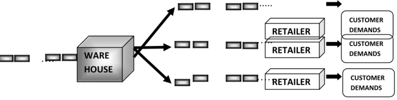
Consider a two echelon, one-warehouse multi-retailer inventory system. It is to be noted that each day, a stochastic demand materializes at each node and unfulfilled demand is backlogged. To fulfill the expected demand, retailers observe their own inventory level, communicate and make decisions whether to reorder or not from ware house. At each store the ordered quantities and the inventory may not exceed storage capacity. Reordering occurs by means of a single track which serves all the retailers,
and set up costs are shared among all retailer who reorders also called ACTIVE RETAILERS. This motivates a certain coordination of reordering policies. It is explained in the below figure:
... ….. …. ……
Fig. 1. One-warehouse multi-retailer inventory system
Decentralization of policies under partial information is mainly focused by Fransoo, Wouters and de Kokin 2001. Yu, Yan and Cheng in 2002 analyze the benefits of the information sharing on the performance of the entire chain. In 2001, Axsater discussed the issues, regarding the use of different kinds of penalties, transfer prices and cost sharing schemes to improve the coordination of policies optimized on a local basis. In 2003, Bauso, Giarre and Pesenti introduced a static context (for fixed day and fixed inventory levels), Saber and Murray in 2003 distributed a consensus protocol for estimating the number of active retailers and coordinating the reordering policies. Each retailer is assumed to choose a fixed threshold policy, with threshold on the number of active retailers, i.e., one defines its intention to reorder only if at least other retailers are willing to do the same.
In this paper we extend the aforementioned results to a dynamic inventory control context in which each day, the inventory levels changes. We prove that a optimal policy, for each i-th retailer, is to order only in conjunction with at least other retailers and also that the threshold can be computed locally by the k-th retailer depending on the current inventory level and expected demand, which is possible by implementing a distributed Neuro-Dynamic
Programming (NDP) algorithm polynomial on the number of retailers, which avoid the curse of dimensionality and reduces errors due to model uncertainties.
In this paper, for a cooperative inventory control problem we develop a hybrid model. Further we prove that the cost-function is k-convex and hence can be efficiently computed in a reduced number of points and also we show that threshold policies on the number of active retailers are optimal. We also introduced the NDP algorithm.
2. HYBRID MODEL
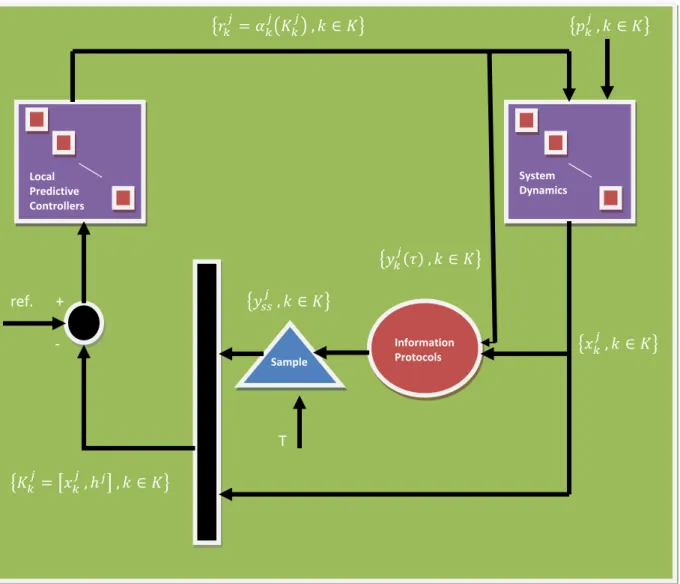
We introduced a novel hybrid model for the multi-retailer inventory system, which is explained in Figure2.
Fig 2. Block Diagram of the closed loop inventory system.
Under the SYSTEM DYNAMICS, we model the n decoupled inventory subsystems. Under the CONSENSUS PROTOCOLS, we model the information flow among the subsystems and
ref. +
-
T
Local
Predictive Controllers
System Dynamics
under the LOCAL PREDICTIVE CONTROLERS; we introduce the structure of the local controllers.
2.1. SYSTEM DYNAMICS
Let us consider a network , where each is a node representing retailer for and each edge representing communication link for
. Let , where is the cardinality of the set S. The model input is the quantity of inventory ordered by the kth retailer at each stage . We model with the stochastic demand faced by the kth retailer. The kth inventory subsystem is a finite-state discrete-time model, that for all takes on the form
.
The inventory at hand plus inventory ordered may not exceed storage capacity as is expressed in the following equation:
, referred to as sensed information is , which means each retailer observes only his inventory level.
2.2. CONSENSUS PROTOCOLS
Through a distributed protocol, the information flow is managed and is given as:
Where , describes the dynamics of the transmitted information of the kth node as a function of the information both available at the node itself and transmitted by the other nodes eq(1). generates a new transmitted information vector given its output at the stage j eq(2). And
estimates, that which is based on current information and having the aggregate information eq(3).
represents the steady state value assumed by within the interval . For a
full state vector the converging value of the transmitted
information, , plus the sensed information, constitute the partial information vector,
available to the kth retailer.
2.3. LOCAL PREDICTIVE CONTROLLER
Over a finite horizon, the local controllers compute the following cost
where is the predicted information and is the discount factor at stage j. The stage cost
is defined as:
Where J represents the set up cost, is the purchase cost per unit stock, is the penalty on storage, is the penalty on shortage and is zero if the kth retailer does not reorder, and one if he reorders.
The algorithm that is used for solution is to taken due to the consideration of simulation-based tunable predicator of the form:
(7)
The set up cost is equally shared among the active retailers, we assumed this in eq(6).
Under consideration we give the formalization of the problem. For a given set of reviewed retailers as dynamic agents of a network with topology G = (V, E).
Problem
, that minimizes the n-stage individual pay off defined in (3).
: (Local Controllers Synthesis) For each kth retailer, determine the reordering
policy
Sub Problem : (Protocols Design) Determine a distributed protocol which maximizes the
3. DYNAMIC PROGRAMMING APPROACH
For the upcoming days, to fulfill exactly the expected demand, the inventory must be ordered in quantity. Let be the set up cost charged to each retailer that reorders at stage j , and
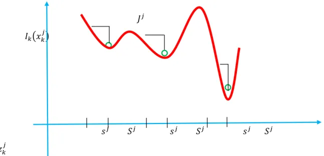
be the instantaneous inventory position (the inventory level just after the order has been issued). Let us consider that if the set up cost decreases with time retailers place short term orders. Optimal policies are multi period policies , with a unique lower and upper threshold which can be easily seen in figure 3.
Fig. 3. Intuitive plot of the cost
On the contrary, if the set up cost increases with time, retailers place long-term orders. Optimal policies are multi period policies with multiple thresholds at different inventory levels which can be easily seen in figure 4.
Fig. 4.Intuitive plot of the cost when the set up cost increases with time : multiple
3.1. SEARCHING FOR STRUCTURE
We first apply the Dynamic Programming (DP) algorithm given by eq (6) and (7) to minimize the cost (5) which shows that the individual objective functions
have atmost n local minima. By defining a new function in which is the maximum set up cost incurred by the kth retailer over the horizon which is obtained by rearranging the Bellman’s equation eq(4) can also be arranged as:
With the help of DP algorithm, we get
Consider a new function as:
Eq.(7) i.e., Bellman’s equation can also be written as:
It is to be noticed that Bellman’s eq.(8) has a unique minimize if we can show that is
-convex then is also -convex. This shows a sufficient condition that guarantees
optimality of multi period order-up-to policies. As we know that represents the minimum threshold on inventory level below which retailers reorder to restore level and
also that minimize and threshold verifies
Let us consider the following:
• as the threshold computed if all retailers would share equally the set up costs ,
namely one nth of the entire cost J.
• as the threshold which corresponds to the assumption that the kth retailer is charged
the whole set up cost; we have .
• In the function , we explicit dependence of threshold on set up cost for
On considering parameter, we show that the individual objective function,
which is a non-convex and has all local minima coincide with the demand summed over one or more days.
Theorem 3.1.1: Solution of the Bellman’s eq.(9) are at most n – j different multi period policies
, where and threshold verifies
. Policy are associated to different intervals of inventory levels.
Proof: Since the cost is piecewise linear, the Bellman’s eq. where the cost is the
summation of a piecewise linear stage cost having unique global minima at and a piecewise linear future cost having potential local minima at .
3.2. THRESHOLD REORDERING POLICIES : Now we have to show that on the
number of retailers interested in reordering, Nash equilibrium reordering policies have a threshold structure. For this we have the following mentioned lemma:
Lemma 3.2.1 : (Single-Stage Optimization) a threshold , for each
inventory level such that the reordering policy
is a Nash equilibrium for the single-stage formulation of the Multi-retailer Inventory Control Problem.
Proof: We have a unique multi period policy from the theorem 3.1.1. Then the
retailers make decision according to the following equation:
To find the minimum value of , for given , that verifies the condition . This is straight forward for the two limit cases of “low” inventory level and “high” inventory level . This lemma can be extended to the multi-stage formulation.
Theorem 3.3.2 : (Multi-Stage Optimization) a threshold for each
is a Nash equilibrium for the multi-stage formulation of the Multi-retailer Inventory Control problem.
Proof : Proof for this theorem is the same as for the single-stage inventory problem in lemma
3.2.1. From theorem 3.1.1, we have at most n – j different multi period policy , each one associated to a different interval of inventory levels. After repeating the above argument for each interval, we get the proof. Optimizing the multi-retailer inventory control problem over a multi-stage horizon leads to Nash equilibrium reordering policies with threshold structure on the number of active retailers.
3.3. LOCAL ESTIMATION WITH CONSENSUS PROTOCOLS
Here we discuss the solution of the sub problem on protocol design and concentrate on consensus protocols to estimate the number of active retailers . Also for a given vector , collecting the optimal thresholds, each retailer makes the decision “do not reorder” if his local estimation is lower than his threshold, as expressed in eq.(13). We assume that the current estimate of the percentage of retailers who are interested in reordering is the transmitted information. At the beginning of each time interval based on the current inventory level , the current estimate is reinitialized to {0, 1}. Also if the corresponding threshold does not exceed the network size n that is the kth inventory level is “low”, then the retailer is willing to reorder, got no information yet except his observed inventory level thus he assumes that all other retailers are in the same circumstances and set , which signifies that today everyone is interested in reordering. On the other hand, if the inventory level is “high” i.e., if exceed n then he is not willing to join the group to order and set , which signifies that no one is in need to reorder. Hence we have
be activated only one time and only when the all local estimates have reached consensus on a final value. This occurs every , where is an estimate of the worst case possible setting time of the protocol dynamics. For a given eq.(14), the continuous-time average-consensus protocol takes on the form:
where L is the Laplacian matrix of the communication network topology; is in turn the time instant where the current estimate converges to a value below the threshold; it can be defined by the following logic conditions such that:
4. NDP SOLUTION ALGORITHM
Here we consider the hybrid model in the field of neuro-dynamic programming.
4.1 CONSENSUS ON FEATURES
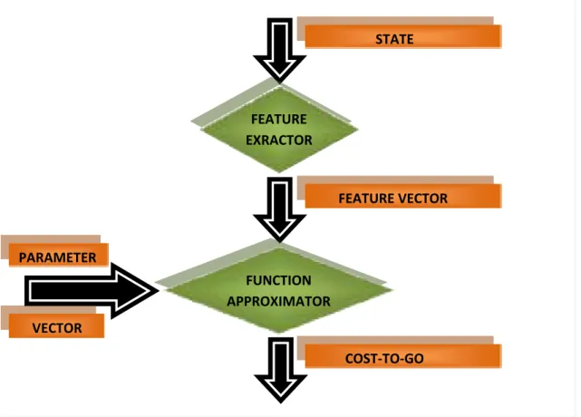
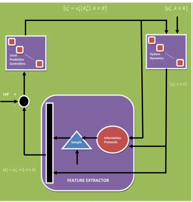
The NDP architecture based on feature extraction displayed in figure 5.
Fig. 5: The information flow management uses consensus protocols to extract the features.
FEATURE EXRACTOR
STATE
COST-TO-GO FEATURE VECTOR
PARAMETER
VECTOR
The block diagram of the Hybrid Model is displayed in figure 6.
+
-
T
Fig. 6 : Block Diagram of the closed loop system
It is to be noticed that the full state vector of the hybrid model, in the approximation architecture, the input to the feature extractor. The information flow management block can be reviewed as the feature extractor. The full state vector reduces to the partial information vector available to the kth retailer. Each local controller implement a function approximation, which receive the partial information vector and returns the individual cost-to-go over the horizon.
ref +
-
Local
Predictive Controllers
System Dynamics
FEATURE EXTRACTOR
4.2. LINEAR ARCHITECTURE
Let us consider that the probability distribution over all potential values assumed by propogates according to the linear dynamics where
. For this we have a matrix of weight q that coincides with the transition probability matrix of the predictor i.e. and basis
functions representing different future costs associated to different . Association of all possible behavior of the other retailers over the horizon, the approximation architecture linearly parameterizes the future costs as:
, where, is the row of the
transition probabilities from to all possible and is the transposed row of the associated future costs.
4.3. THE NDP ALGORITHM
The NDP algorithm consists of two parts. In the first part, the retailers compute the set of admissible decisions and reachable states over the horizon and the second part involving three steps:
STEP 1: Policy Improvement
For a given prediction, we improve the policy with the stochastic Bellman’s equation backwards in time
STEP 2 : Value Iteration
The improved policy is valued through repeated Quasi-Monte Carlo simulations. Active exploration guarantees that initial states are sufficiently spread over the local minima. During the value iteration we compute and store the number of times a transition occurs during the repeated finite length simulations. At the end of each simulation, the protocol runs over the horizon and returns the training set for the next step.
STEP 3. Temporal Difference
We use the training set to update the transition probabilities of the predictor.
Above mentioned three steps are iteratively repeated to get the convergence of policies.
Lemma 4.3.1: Each iteration of the NDP algorithm, for given initial state , has
i
ω1 4 8 6 5 7 8 4 5 6 8
ω2 0 0 1 7 8 0 6 2 1 4
ω3 0 3 2 0 3 1 1 3 3 0
Proof: The proof starts from considering that the complexity of the algorithm depends
essentially on the complexity of the second part. Here, we write the Bellman’s equation considering the set of feasible decisions , for each retailer , for each
stage j = 1, 2, ..., N and for each decomposed state . Thus the complexity is .
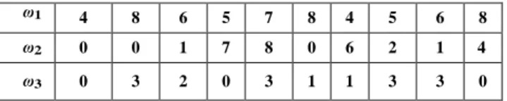
Example 1: Let us consider a group of three retailers and parameters K = 24, p = 8, h =
1, and c = 2. Retailers face a stochastic poissonian demand with expected values over the horizon of ten days as in Table I.
Table 1. Expected demand for the upcoming ten days
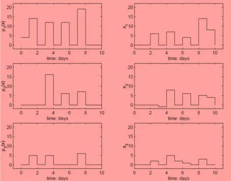
At the first iteration, no communication has occurred among the retailers and the
“policy improvement” returns the uncoordinated reordering policies displayed in Fig.
7.
Fig. 7. Uncoordinated reordering policies
The “value iteration” consists in 12 simulations of the inventory system under the
improved reordering policies. The set of initial states is a stochastic sequence
and 6 for the 1st, 2nd, and 3rd retailer. Indeed, we know from deterministic simulation
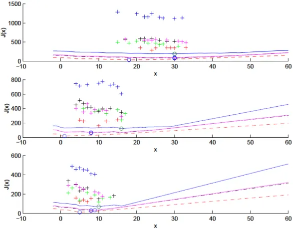
results that J1 has potential local minima at 18, 23, 30, J2 at 1, 8, 16, and J3 at 8, 10 as
displayed in Figure 9 (solid and dotted lines). Here, the costs associated to the 1st, 2nd,
3rd and 4th policy improvements when demand is deterministic are represented by four
lines of different colors (blue, red, magenta, and red). At the end of each simulation
the retailers run a consensus protocol returning akover the horizon. Based on this new
aggregate information, during the “temporal difference” the retailers update the
transition probabilities of the predictor and a new iteration starts. In this example, the
algorithm eventually converges to Nash equilibrium in six iterations returning a
coordinated distribution of reorders
over the horizon as shown in Fig. 8. We see from Fig. 9 that the costs-to-go at the 4th
and 5th iteration (green and red crosses) draw much near to the cost-to-go of the
deterministic problem. We may conclude that the NDP algorithm possesses satisfying
learning capabilities.
Fig. 9. Costs versus inventory : deterministic (colored lines) and stochastic demand (colored crosses)
5. RESULT
We propose an NDP approach to coordinate the reordering policies of a group of
retailers. Coordination is motivated by the possibility of sharing set up cost when
orders are placed in conjunction, therefore we develop a hybrid model to describe the
inventory subsystems and the information flow and designed consensus protocols for
the information flow to presented a scalable and suboptimal NDP algorithm.
REFERENCES
[1]. S. Axs¨ater, “A framework for decentralized multi-echelon inventory control”,
IIE Transactions, vol. 33, no. 1, 2001, pp. 91-97.
[2]. D. Bauso, “Cooperative Control and Optimization: a Neuro-Dynamic
Programming Approach”, Ph. D. Thesis Universit`a di Palermo, Dipartimento di
[3]. D. Bauso and L. Giarr`e and R. Pesenti, “Distributed Consensus Protocols for
Coordinating Buyers”, Proc. of the IEEE Conference on Decision and Control, Maui,
Hawaii, Dec. 2003.
[4]. D. P. Bertsekas, Dynamic Programming and Optimal Control, 2nd ed. Bellmont,
MA: Athena, 1995.
[5]. D. P. Bertsekas and J. N. Tsitsiklis,“Neuro-Dynamic Programming”, Athena
Scientific, Bellmont, MA, 1996.
[6]. J. C. Fransoo, M. J. F. Wouters and T. G. de Kok, “Multiechelon multi-company
inventory planning with limited information exchange”, Journal of the Operational
Research Society, vol. 52, no. 7, Jul. 2001, pp. 830-838.
[7]. R. Olfati Saber and R. M. Murray, “Consensus Protocols for Networks of
Dynamic Agents”, Proc. of American Control Conference, Denver, Colorado, Jun.
2003.
[8]. H. E. Scarf, “Inventory Theory”, Operations Research, vol.50, no.1, Jan-Feb
2002, pp.189-191.
[9]. H. E. Scarf, “The Optimality of (s; S) Policies in the Dynamic Inventory
Problem”, Mathematical Methods in the Social Sciences, Stanford University Press,
Stanford, CA, 1995.
[10]. Z. Yu, H. Yan and T. C. E. Cheng, “Modelling the benefits of information
sharing-based partnerships in a two-level supply chain”, Journal of the Operational
Research Society, vol. 53, no. 4, Apr. 2002, pp. 436-446.