Results of Archaeogeophysical Surveying at
the Great Friends Meeting House in Newport,
Rhode Island
Prepared for:
Cultural and Historic Preservation Program
Salve Regina University
100 Ochre Point Avenue
Newport, RI 02840
and
The Newport Historical Society
82 Touro Street
Newport, RI 02840
Prepared by:
John Steinberg,
Brian N. Damiata, John W. Schoenfelder,
Kathryn A. Catlin, & Christine Campbell
Table of Contents ... i
List of Figures ... i
List of Tables ... iii
Fiske Center for Archaeological Research ... iv
Acknowledgements ... v
Abstract ... vi
Introduction ... 1
GPS & Total Station ... 1
Archaeogeophysics ... 2
Ground Penetrating Radar ... 4
Electromagnetics ... 5
Resistivity ... 6
Interpretations ... 7
Features ... 7
Graves ... 8
Recommendations ... 10
Figures ... 11
Tables ... 78
Bibliography ... 80
Appendix 1 – Georeferenced air photos ... 84
Appendix 2 – Survey Points ... 90
List of Figures
Figure 1. Location of the Great Friends Meeting House. ... 11
Figure 2. 2008 georefrenced air photo. ... 12
Figure 3. Topographic points. ... 13
Figure 4. General Topography. ... 14
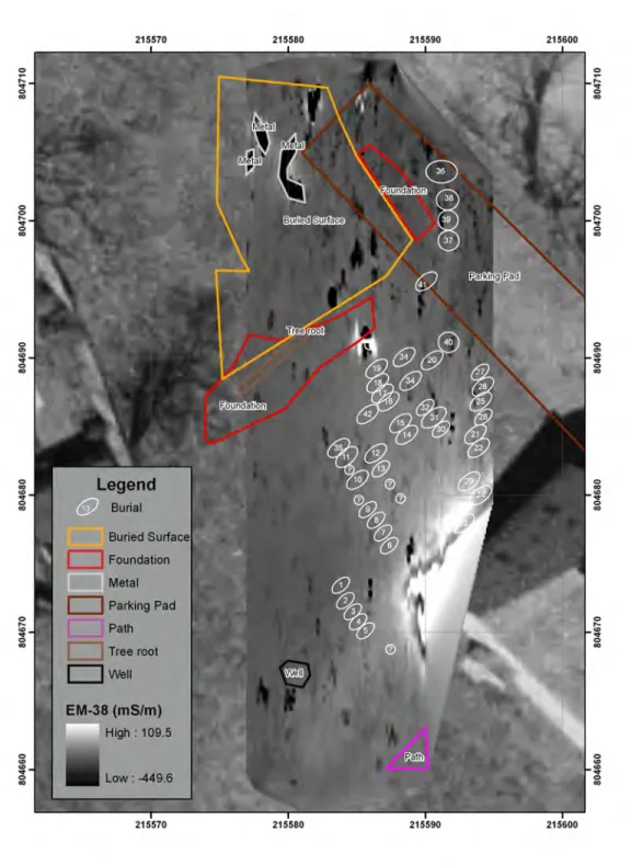
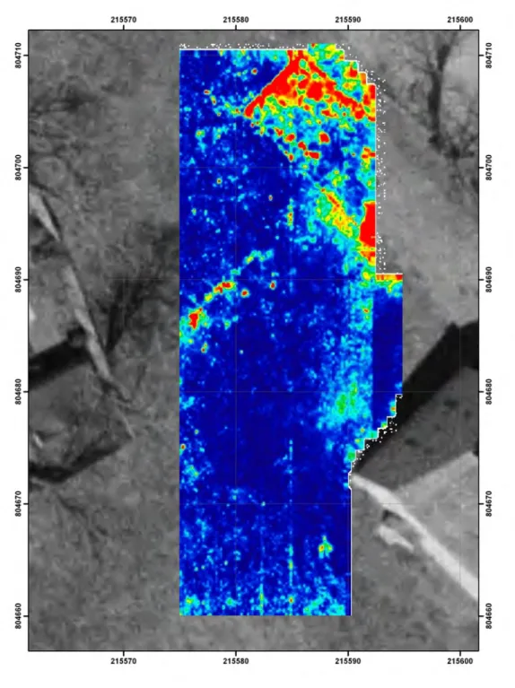
Figure 5. Apparent ground conductivity readings (Q) in black and white scale. ... 15
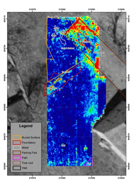
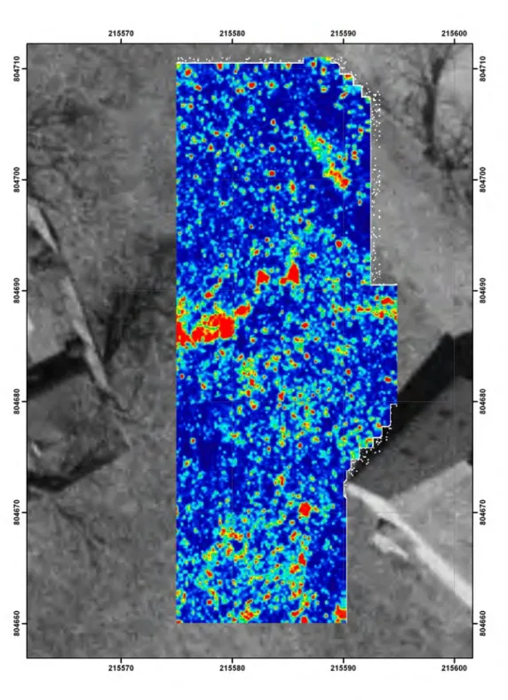
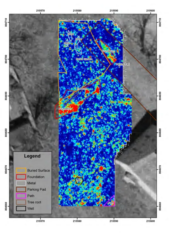
Figure 6. Apparent ground conductivity readings in color scale. ... 16
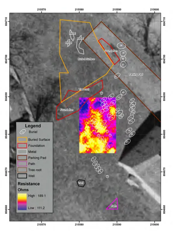
Figure 7. Resistance in color scale (ohm) showing graves and other features identified in GPR.
... 17
Figure 8. Close up showing resistance in color scale (ohm) showing graves identified in GPR. 18
Figure 9. GPR slice 1 of the 500 MHz data at 0-‐7 cm bgs. Strong reflectors are in red. ... 19
Figure 10. GPR slice 1 of the 500 MHz data at 0-‐7 cm bgs. Strong reflectors are in red.
Suggested features are outlined. ... 20
Figure 11. GPR slice 2 of the 500 MHz data at 4-‐11 cm bgs. Strong reflectors are in red. ... 21
Figure 12. GPR slice 2 of the 500 MHz data at 4-‐11 cm bgs. Strong reflectors are in red.
Suggested features are outlined. ... 22
Suggested features are outlined. ... 26
Figure 17. GPR slice 8 of the 500 MHz data at 24-‐32 cm bgs. Strong reflectors are in red. ... 27
Figure 18. GPR slice 8 of the 500 MHz data at 24-‐32 cm bgs. Strong reflectors are in red.
Suggested features are outlined. ... 28
Figure 19. GPR slice 10 of the 500 MHz data at 32-‐39 cm bgs. Strong reflectors are in red. ... 29
Figure 20. GPR slice 10 of the 500 MHz data at 32-‐39 cm bgs. Strong reflectors are in red.
Suggested features are outlined. ... 30
Figure 21. GPR slice 12 of the 500 MHz data at 39-‐46 cm bgs. Strong reflectors are in red. ... 31
Figure 22. GPR slice 12 of the 500 MHz data at 39-‐46 cm bgs. Strong reflectors are in red.
Suggested features are outlined. ... 32
Figure 23. GPR slice 14 of the 500 MHz data at 46-‐53 cm bgs. Strong reflectors are in red. ... 33
Figure 24. GPR slice 14 of the 500 MHz data at 46-‐53 cm bgs. Strong reflectors are in red.
Suggested features are outlined. ... 34
Figure 25. GPR slice 16 of the 500 MHz data at 53-‐60 cm bgs. Strong reflectors are in red. ... 35
Figure 26. GPR slice 16 of the 500 MHz data at 53-‐60 cm bgs. Strong reflectors are in red.
Suggested features are outlined. ... 36
Figure 27. GPR slice 18 of the 500 MHz data at 60-‐67 cm bgs. Strong reflectors are in red. ... 37
Figure 28. GPR slice 18 of the 500 MHz data at 60-‐67 cm bgs. Strong reflectors are in red.
Suggested features are outlined. ... 38
Figure 29. GPR slice 20 of the 500 MHz data at 67-‐74 cm bgs. Strong reflectors are in red. ... 39
Figure 30. GPR slice 20 of the 500 MHz data at 67-‐74 cm bgs. Strong reflectors are in red.
Suggested features are outlined. ... 40
Figure 31. GPR slice 22 of the 500 MHz data at 74-‐81 cm bgs. Strong reflectors are in red. ... 41
Figure 32. GPR slice 22 of the 500 MHz data at 74-‐81 cm bgs. Strong reflectors are in red.
Suggested features are outlined. ... 42
Figure 33. GPR slice 23 of the 500 MHz data at 77-‐85 cm bgs. Strong reflectors are in red. ... 43
Figure 34. GPR slice 23 of the 500 MHz data at 77-‐85 cm bgs. Strong reflectors are in red.
Suggested features are outlined. ... 44
Figure 35. GPR slice 24 of the 500 MHz data at 81-‐88 cm bgs. Strong reflectors are in red. ... 45
Figure 36. GPR slice 24 of the 500 MHz data at 81-‐88 cm bgs. Strong reflectors are in red.
Suggested features are outlined. ... 46
Figure 37. GPR slice 25 of the 500 MHz data at 84-‐92 cm bgs. Strong reflectors are in red. .... 47
Figure 38. GPR slice 25 of the 500 MHz data at 84-‐92 cm bgs. Strong reflectors are in red.
Suggested features are outlined. ... 48
Figure 39. GPR slice 26 of the 500 MHz data at 88-‐95 cm bgs. Strong reflectors are in red. .... 49
Figure 40. GPR slice 26 of the 500 MHz data at 88-‐95 cm bgs. Strong reflectors are in red.
Suggested features are outlined. ... 50
Figure 41. GPR slice 28 of the 500 MHz data at 95-‐102 cm bgs. Strong reflectors are in red. ... 51
Figure 42. GPR slice 28 of the 500 MHz data at 95-‐102 cm bgs. Strong reflectors are in red.
Suggested features are outlined. ... 52
Figure 43. GPR slice 30 of the 500 MHz data at 102-‐109 cm bgs. Strong reflectors are in red. ... 53
Figure 44. GPR slice 30 of the 500 MHz data at 102-‐109 cm bgs. Strong reflectors are in red.
Suggested features are outlined. ... 54
Figure 45. GPR slice 32 of the 500 MHz data at 116-‐124 cm bgs. Strong reflectors are in red. .... 55
Figure 50. GPR slice 40 of the 500 MHz data at 137-‐145 cm bgs. Strong reflectors are in red.
Suggested features are outlined. ... 60
Figure 51. GPR slice 44 of the 500 MHz data at 151-‐159 cm bgs. Strong reflectors are in red. .... 61
Figure 52. GPR slice 44 of the 500 MHz data at 151-‐159 cm bgs. Strong reflectors are in red.
Suggested features are outlined. ... 62
Figure 53. GPR slice 48 of the 500 MHz data at 165-‐173 cm bgs. Strong reflectors are in red. ... 63
Figure 54. GPR slice 48 of the 500 MHz data at 165-‐173 cm bgs. Strong reflectors are in red.
Suggested features are outlined. ... 64
Figure 55. GPR slice 52 of the 500 MHz data at 180-‐187 cm bgs. Strong reflectors are in red. .. 65
Figure 56. GPR slice 52 of the 500 MHz data at 180-‐187 cm bgs. Strong reflectors are in red.
Suggested features are outlined. ... 66
Figure 57. GPR slice 15 of the 800 MHz data at 66-‐73 cm bgs. Strong reflectors are in red
Suggested features are outlined. ... 67
Figure 58. GPR slice 16 of the 800 MHz data at 71-‐77 cm bgs. Strong reflectors are in red
Suggested features are outlined. ... 68
Figure 59. GPR slice 17 of the 800 MHz data at 75-‐81 cm bgs. Strong reflectors are in red
Suggested features are outlined. ... 69
Figure 60. GPR slice 19 of the 800 MHz data at 84-‐90 cm bgs. Strong reflectors are in red
Suggested features are outlined. At this bottom slice, there is substantial north-‐south
line noise. ... 70
Figure 61. Overlay of the hardest reflectors (in red) from 63 to 99 cm bgs. ... 71
Figure 62. Radargrams E595 to 591.2. ... 72
Figure 63. Radargrams E591 to 587.4 ... 73
Figure 64. Radargrams E587.2 to 583.4. ... 74
Figure 65. Radargrams E583.2 to 579.4 ... 75
Figure 66. Radargrams E579.2 to 575.4. ... 76
Figure 67. Radargrams E575.2 to 575. ... 77
Figure 68. 1939 georeferened air photo. ... 84
Figure 69. 1951 georeferenced air photo. ... 85
Figure 70. 1962 georeferenced air photo. ... 86
Figure 71. 1972 georeferenced air photo. ... 87
Figure 72. 1981 georeferenced air photo. ... 88
Figure 73. 2004 georefrenced color air photo. ... 89
List of Tables
Table 1. GPS points. ... 78
Table 2. Possible Grave Listing. ... 78
Table 3. Survey points taken from total station. ... 90
Fiske Center for Archaeological Research
The Andrew Fiske Memorial Center for Archaeological Research at the University
of Massachusetts Boston was established in 1999 through the generosity of the late
Alice Fiske and her family as a living memorial to her late husband Andrew. The
Fiske Center was formally known as the Center for Cultural and Environmental
History.
As an international leader in interdisciplinary research, the Fiske Center promotes
a vision of archaeology as a multi-‐faceted, theoretically rigorous field that
integrates a variety of analytical perspectives into its studies of the cultural and
biological dimensions of colonization, urbanization, and industrialization over the
past thousand years in the Americas and the Atlantic World. Intellectually the
Center staff is committed to building a highly integrated archaeology that
embraces the multiplicity of methodological and theoretical approaches the field
offers. As part of a public university, the Center maintains a program of local
archaeology with a special emphasis on research that meets the needs of cities,
towns, and Tribal Nations in New England and the greater Northeast. The Fiske
Center also seeks to understand the local as part of a larger Atlantic World.
Acknowledgements
James Garman and Catherine Zipf arranged for this work on behalf of Sarah
Schofield, as part of her honors thesis in Culturel and Historic Preservation at
Salve Regina University. The work was permitted by Ruth Taylor, Executive
Director of the Newport Historical Society. John Steinberg obtained the GPS
(Global Positioning System) points. John Steinberg, Sarah Schofield, Catherine
Zipf and James Garman specified the location and position of the survey grid. John
Schoenfielder mapped the surface features and set out the corners of the survey
grid. Brian Damiata, Kathryn Catlin, Christine Campbell, Sarah Schofield, and John
Steinberg carried out the archaeogeophysical surveys. John Steinberg and Brian
Damiata are responsible for the quality control of the survey interpretation of the
data.
None of the suggestions or recommendations in this report should be construed as
geological interpretations (although Brian Damiata is a licensed geophysicist in the
State of California). Rather, these are archaeological interpretations of shallow
geophysical data, in reference to previous excavations whenever possible. The
interpretations presented herein should be ground truthed with targeted
archaeological excavations. The interpretations and assessments are the
responsibility of John Steinberg.
Abstract
Archaeogeophysical surveys were carried out in October 2010 over a 30 x 50 m grid
that was established immediately to the north and west of the north end of the
Great Friends Meeting House (GFMH) in Newport, RI. The surveys were
conducted using a Geonics EM-‐38 RT ground conductivity meter and a Malå X3M
Ground Penetrating Radar (GPR) system that was equipped with 500 and 800 MHz
antennas. In addition, a resistance survey was performed over a much smaller
central area using a Geoscan RM15 resistance meter. From this work three types of
geophysical anomalies have been identified: those associated with individual
features, structures, and graves. There may be one large structure to the north of
the GFMH with a similar alignment. Forty-‐two anomalies were identified that are
consistent with graves. There are many more anomalies that have not been
specifically interpreted as graves because they did not meet enough of our criteria
but may indeed be graves. We recommend that additional archaeogeophysical
surveys be performed as well as a series of follow-‐up excavations to ground truth
the interpretations.
Introduction
There has been an unreported series of excavations near the northern end of the
Great Friends Meeting House (GFMH; Figure 1). Recollections suggest that several
bodies had been excavated near the north end and perpendicular to the long
dimension of the GFMH. Could there be significant geophysical anomalies around
the GFMH that are consistent with graves? If so, how many interments could there
be and what is the spatial extent covered by them?
In an attempt to non-‐invasively assess the number and extent of the unmarked
graves, in the middle of October 2010, we applied Ground Penetrating Radar (GPR)
and electromagnetic (EM) geophysical methods to the area north and west of the
GFMH, as these two methods are commonly used to detect graves (e.g., Bevan
1991). Additionally, Sarah Schofield under the guidance of James Garman,
collected ground resistance data over a smaller central section of the region.
GPS & Total Station
When preforming archaeogeophysical surveys, quality control (QC), is critical and
involves constant attention to instrument calibration, consistency in use, and
instrument recording location. We find that the most important QC parameter is
the accuracy of the geophysical survey grid. Geophysical readings must be
associated with a very specific location that is accurate and reproducible for the
readings to be useful. Slight differences between the actual location of a
geophysical reading and the coordinate assigned during survey can weaken or
eliminate archaeogeophysical signatures. Inaccurate surveying can also create
anomalies where there are none. The effects of inaccurate surveying are magnified
when the data is post-‐processed and filtered.
In anticipation of the geophysical survey, we established three Global Positioning
System (GPS) points using a Trimble GeoXH with a Zepher antenna. At each
location over 600 readings were collected (in three groups of 200 at 5-‐second
intervals) to establish the point. These 600+ readings were then averaged (Table
1). Two of the GPS points (Fairwell & Marb) were accurate enough to be used as
resectioning points for the subsequent land surveying which used the Topcon
GPT9005 robotic total station, that was set up midway between these two GPS
points. The two points were then remeasured and now serve as semi-‐permanent
benchmarks on the Massachusetts State Plane system. These points are described
in Appendix 2 and shown in Figure 2.
With benchmarks established, significant features in the yard were measured (e.g.,
trees, steps, fences). A larger scale topographic grid was established over the
entire yard with points measured in at least every 5 meters (m). In areas of
significant relief, such as close to the house, the topographic points were measured
closer together (see Figure 3). These points are listed in Appendix 2.
Using the Massachusetts State Plane, we established a geophysical grid between
East 215570 to East 215600 and North 804660 to North 804710. Within this 30 x 50
m area, PVC flags were positioned with the Topcon GPT9005 every 10 m whenever
possible. Along the northern and southern sides of this grid, a measuring tapeline
was laid and PVC flags of various colors were placed at integer meter points of the
grid. Every even meter, odd meter, 5 m, and 10 m location had a specific color.
These colored flags were used as endpoints for the north-‐south transects traversed
in the archaeogeophysical surveys. In general, we refer to coordinates within the
GFMH area using the last three digits of the Massachusetts State Plane system. If
no cardinal directions are specified, the order is East, North, and Elevation (X, Y,
and Z). Note that none of the archaeogeophysical surveys that were performed
(GPR 500, GPR 800, EM-‐38, & resistivity) surveyed exactly the same area, but all
focus on the areas to the north and the northwest of the northern end of the
current GFMH.
Archaeogeophysics
Archaeogeophysics is the application of non-‐destructive geophysical methods and
principles to archaeological settings. More specifically, archaeogeophysics
involves the interpretation of geophysical signatures (anomalies) that may be due
to buried archaeological sites and features. In some cases, archaeological features,
subsurface geology, graves, and sometimes artifacts and ecofacts can be located
and partially analyzed based on their geophysical signatures. Shallow geophysical
surveying has been particularly useful in understanding landscape features such as
gardens (Cole, et al. 1997; Yentsch and Kratzer 1994) and cemeteries (Jones 2008;
King, et al. 1993) that cover a large area and cannot be completely excavated.
Archaeogeophysics is not an exact science. We have found that small differences in
the environment (e.g., soil moisture, surface cover, changes in ambient
temperature) can affect geophysical measurements, and therefore change the
nature and shape of the interpreted geophysical anomalies. A geophysical
In archaeogeophysics, the choice of methods, equipment, and field procedures can
have as much or more of an effect on the detection of archaeological features as
the contrasts between the features and the surrounding matrix (Pomfret 2006).
Because the work is non-‐destructive, surveys can, and usually are, performed
multiple times with slightly different parameters in order to obtain the best results
(Kvamme 2006; Kvamme, et al. 2006; Watters 2009).
In general, interpretations based on archaeogeophysical data should be ground
truthed through archaeological excavations. Even small excavations of targeted
geophysical anomalies can greatly enhance the overall accuracy of the
interpretations. Similarly, the archaeogeophysical interpretations can help to guide
the efficient placement of excavations. The reflexive use of archaeology and
geophysics can establish a local geophysical signature for an archaeological
feature. That is, when archaeological investigations are in a feedback loop with
geophysical surveys we can turn a geophysical anomaly into an archaeological
signature.
In some cases, important archaeological features may not produce a sufficient
geophysical contrast with its surroundings to be detected with the methods and
post-‐processing techniques applied herein. The detection of archaeological
features depends on the measurable contrast produced between the background
subsurface characteristics and the archaeological features. The detectability is a
function of size, geometry, depth, and contrast. A given archaeological feature in
one environment may not be detectable in another environment. By collecting a
series of profiles we assess whether there is any geometry associated with an
anomaly and then make an interpretation as to whether the cause is natural or
could be an archaeological feature. Sometimes, contrasts between archaeological
features and the surrounding environment will show up with one method and may
not show up in another. The use of multiple geophysical methods that measure
different physical properties of the subsurface may mitigate this problem.
Sometimes more accurate archaeogeophysical interpretations can be made when
an anomaly only manifests itself with one geophysical method. However,
anomalies that manifest themselves in multiple methods are usually substantial.
Archaeological interpretations based only on geophysical results have their
limitations. While some anomalies are much more suggestive than others, there
are no characteristic anomalies per se (i.e., different types of features can produce
an identical geophysical signature) The most “accurate” interpretations are those
Ground Penetrating Radar
Ground Penetrating Radar (GPR) has become The Fiske Center’s principal
archaeogeophysical method for high-‐resolution mapping of buried architecture
(Neubauer, et al. 2007), cultural deposits (Goodman, et al. 2008; Goodman, et al.
2007), and graves (Doolittle and Bellantoni 2010). In the method, an
antenna/receiver unit pulses microwaves energy as it is towed along the ground
surface. At interfaces that exhibit significant contrasts in dielectric constant—an
electromagnetic property—some of the energy will be reflected back to the
receiver. The longer it takes for the microwaves to return, the deeper the reflector
(all other factors being equal). The more energy a feature sends back, the
“stronger” the reflection. Buried flat rocks, laying parallel to the ground, are some
of the strongest microwave reflectors. Conversely, the presence of saline soils will
absorb the energy and limit depth of penetration (Goodman and Conyers 1997).
Therefore, assuming a deposit is non-‐saline, the reflected pulse contains
information about the nature of the reflectors over a variety of depths (Conyers
2005). In general, the deeper the target, the more difficult it is to detect and the
lower the resolution of the feature.
The strength and time lag of the reflected microwave energy can be plotted to
create a pseudo-‐profile of the intensity of reflectors over the depth, which is called
a Radargram. These can be seen in Figure 62 through Figure 67. In these figures
the black and white bands are the amplitude of the reflected energy (black is the
positive and white is the negative part to the wave). As the depth increases, the
area that receives and reflects the microwaves becomes larger, and therefore, the
signals reflected back to the receiver become even weaker. The raw data are
typically gained to increase the strength of the signals from the lower parts of the
radargram. A series of these pseudo-‐profiles can then be combined and “sliced” at
a given depth to create a plan view of the subsurface reflections. The slices use the
squared amplitude of the wave, making the positive and negative aspects of the
microwave look the same.
In general, the northeast has good suitability for GPR (Doolittle 2009) and
Newport should have good soils for application of the method. However, the
proximity to the sea of the GFMH may mean some attenuation of the GPR signal
due to salt. However, the relatively low apparent ground conductivity measured in
the EM survey (avg. of about 11 mS/m ) would suggest relatively little salt in this
area. Clay can also cause problems for GPR, but the soils around Newport are high
from interfaces and features over 2.1 m below the ground surface (bgs) using the
500 MHz antenna and 90 cm bgs with the 800 MHz antenna. For both GPR
surveys, transects were spaced 20 cm apart across the survey grid and were
traversed unidirectionally. The radargrams were processed with GPR-‐Slice
software (see www.GPR-‐slice.com), using 7 cm slices every 3.5 cm for the 500 MHz
data (60 slices over 2.11 m) and 6.5 cm slices every 4.7 cm for the 800 MHz data (19
slices over 90 cm). In both cases, this provides significant overlap and continuity
between slices, yet gives good resolution (all of these are available on the attached
CD). The raw data is contained in the enclosed CD and can be re-‐sliced at other
depths and thicknesses. In general, this reports only utilizes every other slice.
Electromagnetics
The Geonics EM-‐38 ground conductivity meter emits an alternating current and
measures the strengths of the resulting direct primary magnetic field as well as the
secondary magnetic fields that are generated within the ground (Dalan 1991;
McNeill 1980; Tabbagh 2009). The instrument measures apparent ground
conductivity (in units of milliSiemens per meter, mS/m) that is a function of bulk
ground conductivity. The instrument does not need to be in direct contact with
the ground, and therefore, can be used on rough and undulating terrain. The 1-‐m
coil separation provides for a relatively shallow depth of investigation (< 1.5 m) and
therefore good resolution of changes in apparent ground conductivity close to the
ground surface.
We used an EM-‐38 RT that was manufactured in 2001 and retrofitted for
temperature compensation by Geonics Ltd. in December of 2009. This
modification reduces the sensitivity of the unit to changes in temperature caused
by changes in sun, shade, or ground heat. However, some conductivity changes
may be a response to taking readings with different ambient temperatures.
The EM-‐38 RT can also yield the In-‐Phase component (IP) in parts per thousand.
The IP readings are similar to those of a metal detector and can be thought of as a
field measure of magnetic susceptibility. Unfortunately, the particular model of
the EM-‐38 that we employ (RT) can only record one component at a time. At the
GFMH, we chose to record apparent ground conductivity in hopes of identifying
changes in conductivity associated with burial shafts. We suggest performing a
similar survey with the EM-‐38 and recording the IP component instead.
During the EM-‐38 survey, intermediate base-‐station readings were taken to check
for instrument drift. The base station was established at E 990, N 680. In addition,
a quality control (QC) line was established east-‐west at the N 680 line and could
be used to tie in all of the north-‐south transects. This perpendicular transect was
run before and after the survey. The repeatability of the QC data indicates that the
survey was accurate and reproducible under similar conditions. The results
presented in Figure 5 have not been filtered or smoothed, nor has the small offset
in the data been accounted for.
For the survey, apparent ground conductivity readings were recorded every 5 cm
along north-‐south transects that were spaced 20 cm apart. The transects were
traversed in a unidirectional manner. The apparent ground conductivity ranged
from -‐449 to +109 mS/m, with negative values due to the presence of buried pieces
of metal. The average value is 11.6 mS/m with a SD of 14 mS/m. Most of this
variation seems to be due to the metal (which cause huge positive and negative
swings), possibly associated with a structure (Figure 5). The range of apparent
ground conductivity relevant for the identification of non-‐metallic archaeological
features is from 2 to 25 mS/m (Figure 6).
The results of the conductivity survey were not conclusive. Even with dense
recording and tightly spaced transects, we are not able to detect individual graves.
However, the data does suggest a graveyard area consistent with the overall spatial
extent of graves as identified in the GPR (Figure 30). The general grave area is
indicated by a more variable series of slightly conductive areas marked in blue
(about 17 mS/m). This suggests that the apparent ground conductivity of
disturbed graves is higher than the surrounding intact soil.
Resistivity
The resistivity method measures how well the soil conducts electricity by injecting
a direct current through a pair of electrodes and measuring the Earth’s response
through a second pair of electrodes. The resistivity of the subsurface is a function
of soil moisture, soil texture, concentrations of salts, and presence of ferrous
material. Wet soils with a high clay content and high salt levels provide very good
conductive mediums whereas dry rocky and sandy soils are poor conductors.
The resistivity method is good for assessing resistive targets in a conductive
environment (Gaffney and Gater 2003; Hargrave, et al. 2002; Kvamme 2006;
Garman employed a Geoscan RM15 resistance meter and collected the data. A
current-‐potential spacing of 0.5 m was used, with one set of electrodes remotely
spaced more than 30 m away. Note that the unit provides a measurement of
resistance (units of ohms) as compared to the conventional resistivity method
(units of ohms-‐m).
There appears to be little correspondence in the resistance data compared to the
graves as interpreted with the GPR data (see next section). Grave shafts (the soil
put back into the shaft) can be either resistive or conductive targets even within
the same cemetery (Jones 2008:29). Based on the admittedly disappointing results
from the EM-‐38, we suspect that the grave shafts might be marginally more
conductive than the surrounding intact soil and therefore resistance may not be
the best method to detect graves at the GFMH. Although the general northeastern
trend of the data follows the same orientation of graves as interpreted with the
GPR data (Figure 8), the correspondence between the two data sets is weak.
Interpretations
Features
Most of the interpretive features are located in the northern and northwestern
portions of the surveyed area. No obvious utilities were detected but there may be
a few deep pipes. Important and obvious features include the parking pad, tree
roots, metal pieces, a buried surface, associated foundations, a well, and a path.
The survey was not designed to delineate these suggested features, and therefore
the extent of them may not be completely surveyed.
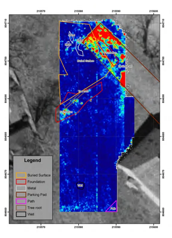
The main feature that may have some effect on the detection of other features is
the stone parking pad in the northeast. This feature is visible in both the
electromagnetic (EM) data and the upper slices of the GPR data. It also may affect
the lower slices by causing an offset of the slices.
Northwest of the grave field is a possible structure. This feature is best observed in
the 500 MHz slices. The combination of a buried surface and shallower linear
features that surround it probably make up part of a structure of some sort, and it
will be described as such hereafter. The foundation shows up in slice 8 (24-‐32 cm
bgs, Figure 18) and is strongest in slice 14 (39-‐46 cm bgs, Figure 24). The southern
part of the foundation area has a particularly strong east-‐west linear feature that
Figure 26). We tentatively interpret this to be a subsurface floor surrounded by a
foundation wall. There may be some pieces of metal associated with structure that
are clearly evident in the EM data (labeled Metal in Figure 6).
There is also part of a path or some utility which the southeastern part of the
survey area just intercepted the corner. This anomaly is labeled “Path” and is first
seen in slice 22 (74-‐81 cm bgs, Figure 32) in the 500 MHz data and is clearly visible
in slice 30 (107-‐110 cm bgs, Figure 43). This same anomaly is also visible on the
deepest slices of the 800 MHz data (slice 19, 84-‐90 cm bgs, Figure 60). In the
southern part of the survey area is a feature labeled “Well.” This is one of the
strongest, most consistent, and deepest anomalies that was encountered. It first
shows up in the in slice 15 (66-‐73 cm bgs, Figure 57) of the 800 MHz data and in
slice 17 (75-‐81 cm bgs,) of the 500 MHz data. Slice 17 is not presented in the figures
but the same anomaly can be seen in slice 18 (Figure 27 & Figure 28).
Possible, but unlabeled features include some sort of buried surface just to the
west of the grave field that occurs at depths of 60-‐73 cm bgs (Figure 57) in the 800
MHz data. Because this does not show up particularly well in the 500 MHz data,
we have not labeled it. Also, on the deeper 500 MHz slices, there are two strong
deep anomalies located 12 m north and northeast of the well (e.g., see Figure 47,
Figure 53, and Figure 55). The nature of these strong deep reflectors is not known
and they do not appear higher up in the sequence. There also may be several deep
pipes, which are not labeled on the slices but can be identified in the radargrams
(e.g., Figure 66)
Graves
Quaker graves are a difficult class of burials to detect (Bromberg and Shephard
2006). GPR can be a very effective method for detecting graves when general
conditions are suitable for use of the method (King, et al. 1993).
Stronger reflectors that arise from the coffin, the body, and the shaft itself will
generally suggest burials. Breaks in the soil stratigraphy and the corresponding
grave shaft fill can also be identified (Jones 2008). In addition, either the sides or
the bottom of the pit can sometimes be detected if the pit has cut through and
disturbed preexisting soil layers (Conyers 2006a:154). Void spaces (e.g., air
pockets) from relatively intact coffins and possibly the skull and chest cavity
(Hammon, et al. 2000) are potential targets but bones are usually too small to be
The orientation of the individual feature reflections is important for identifying
graves. Most obvious in Christian cemeteries is a consistent east-‐west orientation
(Fiedler, et al. 2009). At the GFMH the graves seem to be perpendicular to the
long dimension of the Meeting House. Therefore, if GPR survey is performed
perpendicular to the long axes of the graves, each burial should be identifiable
across several radargrams. In particular, we look for anomalies that appear on
multiple transects that would create a 1.2-‐2.2 m long and 0.4 m wide deep strong
reflector that would result from the remains of the casket or box (Hammon, et al.
2000).
The geometry of a group of reflections is also important for identifying graves.
Most importantly, a linear sequence of separated reflections may imply a series of
graves. In particular, multiple anomalies separated by a meter or so are a strong
indication of burials. Between deep strong reflections there can be strong near-‐
surface reflections that result from foot traffic between graves (Fiedler, et al. 2009).
All of these geometric possibilities are considered when interpreting the existence
and the location of graves.
Because of the complexity of this grave field, we have only identified the most
obvious graves. This means that we have identified the deeper larger burials (or at
least larger grave shafts) and those with the most intact coffins. Therefore, we
have not identified shallower, smaller, and degraded graves. By concentrating on
the most obvious graves, we have been able to outline the burial area and suggest a
general orientation for the more robust graves. This is a conservative approach to
grave identification.
In total, 42 potential graves have been identified within a very well confined area
(see Table 2). These selected anomalies are very good candidates, satisfying
several criteria for graves. We have omitted many shallower anomalies in that
region that are possibly graves. Many of these are just north of the western corner
of the GRMH and can be seen in slice 6 (18-‐25 cm bgs, Figure 15 & Figure 16). The
graves that have been identified and numbered generally begin to appear on slice
18 (60-‐67 cm bgs, Figure 27 &Figure 28) and are most clear on slice 22 (74-‐81 cm
bgs, Figure 31 & Figure 32). These graves show a strong linear anomaly over
multiple slices. Furthermore, all of the identified graves have either a break in the
surface or a phase change in the lower strong reflector. Even with this
conservative approach (each identified grave must have at least one distinct grave
characteristic beyond the geometry) the general burial area becomes apparent.
present good signals, but they are not quite as strong as graves 1-‐5. The separation
of these graves could be an artifact of the grid configuration and the presence of
the parking pad. Figure 61 shows an overlay (Goodman, et al. 2008) where all of
the strongest reflectors from 63 to 99 cm bgs are presented in one image.
Recommendations
The archaeogeophysical results from the Great Friends Meeting House have
provided useful information, and we suggest that more surveys and small targeted
excavations be performed. Specifically, we recommend three more surveys. GPR
survey using the 500 MHz antenna and with transects oriented east-‐west should
be conducted over the grave shaft area to better delineate the buried surface and
associated foundations. We also recommend an EM-‐38 survey over the same area
but recording the IP component along unidirectional transects spaced every 20
cm. This survey might detect individual grave shafts and would provide a
complementary dataset that could be compared with the GPR results that have
been presented herein.
Assuming that the nature of the foundation and buried floor surface is not
documented elsewhere, we also think it very important to perform a GPR survey
over this area. The present survey was designed to detect graves and therefore was
not focused on possible structures located to the northwest of the grave field. We
suggest a complete survey over a larger area (e.g., 50x50 m). This will ensure that
the entire structure and its surroundings are captured.
Finally, we recommend that after the above surveys have been performed and
results examined, that a series of exploratory archaeological excavations into the
major anomalies be carried out. These excavations should be placed so as to
crosscut the major anomalies that have been identified.
Figures
Figure 1. Location of the Great Friends Meeting House.
Figure 2. 2008 georefrenced air photo.
A
A
A
215550.000000 215600.000000 215650.000000 8 0 4 6 0 0 .0 0 0 0 0 0 8 0 4 6 0 0 .0 0 0 0 0 0 8 0 4 6 5 0 .0 0 0 0 0 0 8 0 4 6 5 0 .0 0 0 0 0 0 8 0 4 7 0 0 .0 0 0 0 0 0 8 0 4 7 0 0 .0 0 0 0 0 0 8 0 4 7 5 0 .0 0 0 0 0 0 8 0 4 7 5 0 .0 0 0 0 0 0 8 0 4 8 0 0 .0 8 0 4 8 0 0 .0Legend
Meeting House outline
Figure 3. Topographic points.
215570.000000 215580.000000 215590.000000 215600.000000 215610.000000 8 0 4 6 5 0 .0 0 0 0 0 0 8 0 4 6 5 0 .0 0 0 0 0 0 8 0 4 6 6 0 .0 0 0 0 0 0 8 0 4 6 6 0 .0 0 0 0 0 0 8 0 4 6 7 0 .0 0 0 0 0 0 8 0 4 6 7 0 .0 0 0 0 0 0 8 0 4 6 8 0 .0 0 0 0 0 0 8 0 4 6 8 0 .0 0 0 0 0 0 8 0 4 6 9 0 .0 0 0 0 0 0 8 0 4 6 9 0 .0 0 0 0 0 0 8 0 4 7 0 0 .0 0 0 0 0 0 8 0 4 7 0 0 .0 0 0 0 0 0 8 0 4 7 1 0 .0 0 0 0 0 0 8 0 4 7 1 0 .0 0 0 0 0 0 Legend Topographic Points Elevation asl (m) <VALUE> 6.75 - 6.84 6.85 - 6.9 6.91 - 6.95 6.96 - 7 7.01 - 7.05 7.06 - 7.12 7.13 - 7.17 7.18 - 7.22 7.23 - 7.27 7.28 - 7.33 7.34 - 7.39 7.4 - 7.46 7.47 - 7.52 7.53 - 7.59 7.6 - 7.65 7.66 - 7.7 7.71 - 7.76 7.77 - 7.81 7.82 - 7.86 7.87 - 7.94
Figure 4. General Topography.
215570.000000 215580.000000 215590.000000 215600.000000 215610.000000 8 0 4 6 5 0 .0 0 0 0 0 0 8 0 4 6 5 0 .0 0 0 0 0 0 8 0 4 6 6 0 .0 0 0 0 0 0 8 0 4 6 6 0 .0 0 0 0 0 0 8 0 4 6 7 0 .0 0 0 0 0 0 8 0 4 6 7 0 .0 0 0 0 0 0 8 0 4 6 8 0 .0 0 0 0 0 0 8 0 4 6 8 0 .0 0 0 0 0 0 8 0 4 6 9 0 .0 0 0 0 0 0 8 0 4 6 9 0 .0 0 0 0 0 0 8 0 4 7 0 0 .0 0 0 0 0 0 8 0 4 7 0 0 .0 0 0 0 0 0 8 0 4 7 1 0 .0 0 0 0 0 0 8 0 4 7 1 0 .0 0 0 0 0 0 Legend Elevation asl (m) <VALUE> 6.75 - 6.84 6.85 - 6.9 6.91 - 6.95 6.96 - 7 7.01 - 7.05 7.06 - 7.12 7.13 - 7.17 7.18 - 7.22 7.23 - 7.27 7.28 - 7.33 7.34 - 7.39 7.4 - 7.46 7.47 - 7.52 7.53 - 7.59 7.6 - 7.65 7.66 - 7.7 7.71 - 7.76 7.77 - 7.81 7.82 - 7.86 7.87 - 7.94