Quantifying the Impact of Multiple Risks on Software-Intensive Programs

Quantifying the Impact of Multiple Risks on

Software-Intensive Programs

Sharon A. Els

Kimberly Sklar Reichelt

Kenneth G. Cooper

PA Consulting Group

Cambridge, MA 02142

[sharon.els; kim.reichelt]@paconsulting.com

[email protected]

It is a rare program that is affected by just a single risk. There may be one risk that is of more concern than others, but there are almost always other risks that can compound the challenges and impacts of any single risk. If not foreseen and mitigated, compounding risk impacts can be a dangerous phenomenon. Our findings show that the program impact of a single risk can be significantly greater—by 20–30% or more—when it occurs in the presence of certain other risks.

The authors have developed an approach using system dynamics simulation to assess the impact of both isolated risks and the combined impact of risks. The model employed simulates the primary cost drivers of most programs— staffing, work schedules, the drivers of productivity, and the causes of rework.

This paper focuses on the dynamics that can cause compounding impacts in combinations of potentially interacting risks.

Keywords: System dynamics, simulation, risk analysis, program management, compounding risk impact

1. The Problem of Quantifying Multiple Risks Are there compounding impacts of multiple risks on a program? Can we rely on the adequacy of impact estimates of each individual risk element in isolation? In other words, can the impact of Risk A be greater in the presence of Risk B than if Risk A were to occur alone?

Simulation plays a vital role in this evaluation of risks’ compounding impacts. One cannot easily experiment on an operating program to gauge the impact of various combinations of risks or to determine the existence of or degree of compounding of these risks. The best place for such experimentation is a simulation that can replicate the real program but allow “what if” testing. The use of program simulation enables dispassionate analysis of the causes and magnitude of such impacts; it enables testing to identify the extent of compounding impacts and the circumstances under which compounding impacts occur.

The answers in the evaluation have significant implications for program planning and management.

If compounding impacts are present, different contingent plans would be needed for different combinations of future conditions. Estimates of the probabilities of program cost levels would need to be adjusted. Staffing and executing the work would need to accommodate the altered conditions. Mitigating actions would need to be redesigned. Potential effects on other procurements would need to be flagged proactively. While none of these prospects may seem attractive, advance planning is crucial. In the absence of forewarning, without better understanding of the impact of multiple risks, programs are doomed to be “surprised” by them, without effective preemptive mitigation plans.

The prospect of multiple risks hitting a single program is very real as the list of potential challenges to a program is long.1 _{For example, the risk list for an} individual program may include instances of one or several of the following:

Funding delays

Known or unknown technical challenges •

•

1. See, for example, GAO Report Number 05-301, “Defense Acquisitions: Assessments of Selected Major Weapon

Late or missing information/material

Evolving or changing requirements definition Resource availability problems (computers, people, offices)

Less reuse or lower productivity than planned Increases in work scope

Inadequate domain experience

Shortages of staff and/or competition for resources from other programs

High attrition rates

Excessive reviews and meetings

Problems with subcontractor or partner performance

Delays in performance of related program These risks are both real and common. For example, the risk of facing late or missing information is widespread. The March 2005 GAO report found that “The majority of the programs proceeded with less knowledge at critical junctures than suggested by best practices.” They concluded that this late information had contributed “to large cost growth and schedule delays” [1].

A “compounding” impact can occur when multiple changed conditions combine to produce a total impact that is greater than the sum of the individual changes’ impacts (including their “knock-on” effects2_{)[2]. An example is when one activity is} delayed by a condition (such as late information)— which impacts productivity—and another changed condition separately impacts a different activity (with its own set of knock-on impacts). Together, the two changed conditions may aggravate the total impact of the two individually. For example, if the two changes combine to generate a need for more hiring of new staff, there can easily be a nonlinear impact on the staff productivity, as new hires may not only work less productively but also create increasing demands on supervision, draining the supervisory time available for other problem solving. This added consequence can then trigger further impact, such as allowing additional rework that less-strained supervisors could have avoided—hence, a multi-path compounding impact of the combination of changed conditions. On a program with critical talent needs, this is an all-too-familiar phenomenon and an example of how combined changes can accelerate the

• • • • • • • • • • •

degree of impact significantly beyond the simple sum of individual impacts.

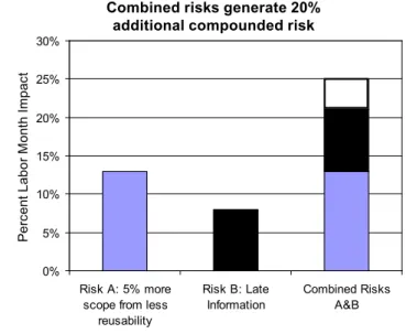
Figure 1 demonstrates analysis results from just such a case, a typical large software project, which is described below. Here, one risk (lower reuse) yields a 13% impact and another (late information from a related program) yields 7%. The impact of the two combined, however, is not 20% but 24%. How and why does this “compounding impact” occur?

It is vital to understand the causality of the phenomena that affect program performance and to be able to analyze compounding impacts, so as to be able to design effective mitigating actions to control those phenomena. Without that foresight and proactive action, any complex program on which there are multiple changing conditions is destined to suffer unanticipated and unmitigated impacts that can significantly harm program performance [3]. 2. The Method

The enabling simulation technology for this work is called system dynamics. A system dynamics model replicates in a computer simulation model the feedback loops that drive real-world performance. Systems dynamics was invented at the Massachusetts Institute of Technology (MIT) in the late 1950s to help government and businesses design durable improvements to complex problems. Professor Jay W. Forrester developed the field of system dynamics by applying what he learned about

Combined risks generate 20% additional compounded risk

0% 5% 10% 15% 20% 25% 30% Risk A: 5% more

scope from less reusability

Risk B: Late

Information Combined RisksA&B

Percent Labor Month Impact

Risk A Risk B Additional Total Impact When Combined

Figure 1. The impact of Risk A and Risk B in combination results in a compounded cost impact which is greater than the sum of the individual cost impacts.

2. By “knock-on” effects we refer to the indirect effects of a

condition, as in the impact of reduced productivity that may

accompany an addition of workscope—the new workscope is a direct effect; but if they cause, for example, additional overtime

that reduces the overall productivity of the work, then the increased hours caused by lower productivity on the new and

existing workscope is the indirect or “knock-on” effect.

Pe rc en t L ab or M on th I m pa ct

Combined risks generate 20% additional compounded risk

systems in his work in electrical engineering and control theory to other kinds of systems involving organizations and complex behavior. What makes system dynamics different from other approaches to studying complex systems is the use of feedback loops. Stocks (accumulations) and flows (rates of change) help describe how a system is connected by feedback loops that create the nonlinearity and resistance to change found so often with complex problems. System dynamics simulation models apply control theory, including feedback and time delays, to represent the dynamics and behavior of complex systems under different conditions.

Over thirty years ago, we built the first project model using system dynamics, and refined and enhanced it since. Over one hundred large programs have used the method and particular model described here, most in top-tier defense contractors. Programs employ this method to simulate program performance and, with a wide range of “what if” tests, examine how changed conditions or management actions would alter cost and schedule performance.

We build and tailor a project model in conjunction with project managers and staff. We collect an extensive set of data describing a project’s scope, budget, and schedule, as well as the labor environment, performance history on the project (if it has already started) in terms of labor applied, progress achieved, initial issues, revisions, overtime used, recollections of program history describing factors that affect productivity, data on change orders, etc. Initial model values are set based on past experience with similar projects in the same industry, are then tailored to reflect information from interviews with project managers and staff, and finally are adapted through an iterative calibration and validation process.3 _{The result of}

this process is a model that accurately captures the dynamics of a specific project, replicating the known history of the project that is already underway, or consistent with the details of a prospective project and tailored based on other similar, completed projects. Our work in project management was first conducted in the late 1970s and published in 1980[6]; and since, we and others have followed with dynamic models describing the impacts of varying productivity on project performance. Tarek Abdel-Hamid has done work focusing on software projects [7]. Susan Howick has focused on the quantification of disruption [8]. Substantial literature has confirmed the presence of individual pieces of the productivity puzzle—how much overtime [9] or weather [10] or change orders [11] affect productivity. But it is only by considering

all these factors in combination that we can get a real handle on the dynamics of a project.

While our project models have been used in a variety of ways before, during, and even after program execution, the focus here is on the proactive evaluation of different risks’ performance impacts. Imagine running a large, complex software-intensive development program. Several distinct teams are working on separate modules, many of which depend on one another. The managers develop plans and, having done this many times before, are careful to include contingencies in both cost and schedule and to consider the many interdependencies among the tasks. The program begins smoothly, but later, when “risk” conditions emerge as actual changes, the managers find it nearly impossible to keep the plans up to date and the work on target. In the test results that follow, we have set up a model of a program with those characteristics—a fictional one, but with realistic parameters, adapted from validated models of large software projects. The analyses that result are consistent with analyses we have run on dozens of real-world, calibrated, tested, and validated models of software projects.

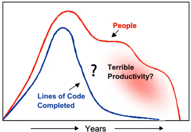
The difficulty for planners and managers is that most planning tools start with two very basic, and usually incorrect, assumptions. They assume, as in Figure 2 below, that (1 ) as you apply people to tasks they will complete these tasks in the planned number of hours, i.e., at a productivity that is constant throughout the task; and (2 ) once done, work is complete and will not need later revision.

Consider our fictional software program manager. Early on, the team may seem to perform ahead of plan, showing favorable variances relative to both planned budget and schedule. But later, it seems little net progress is occurring (Figure 3). Team leaders report that everyone is working as hard as they can, even logging large amounts of overtime, and yet progress estimates are barely budging, sometimes even edging backward. How is this possible?

As programs near completion, it is common for them to suffer a “lost year,” during which every step forward seems to be accompanied by two going backward. To those going through it, it may feel as though external events are the cause—just when things were going so well, the requirements change,

3. Model calibration and validation are beyond the scope of this paper, but have been discussed in earlier papers, e.g.,Lyneis,

Reichelt, and Bespolka [4] and Stephens, Graham, and Lyneis [5]. Figure 2. Productivity may vary as people accomplish work.

PeopleProductivity

Work To

Be Done WorkDone

PeopleProductivity

Work To

or planned reuse turns out to be infeasible, or a schedule milestone is accelerated, or the budget is cut. Most often, however, when we step back and analyze what is really going on, the answer is more systemic. “Rework” is being discovered faster than the staff can fix it. This rework, work which was not done correctly and completely the first time, actually had been accumulating over the preceding months and now, as testing intensifies and problems are found while integrating the modules, it is being discovered (Figure 4). Capers Jones highlights the tremendous cost this rework can have, with rework costs being as high as 60% of the effort for very large projects [12]. Whenever program productivity or rework is affected by a changed condition (and the risk is realized) the cost and/or schedule performance is impacted. The key questions are: By how much? When? In which segments? Why? What improvements can be made? It may be that none of these questions can be answered adequately without considering the compounding impacts of multiple risks.

3. The Dynamics of Compounding Risk

Imagine our software program operating in a relatively tight labor market, one among several programs at its company location. Among these other programs is one on which our program of interest is technically dependent, despite being contractually completely separate. The program is planning a high degree of reuse from a prior effort, but there is a risk that this level of reuse is not attainable.

In the section below, we examine the impact of (a) the program achieving lesser reuse than planned, and (b) late information from the precedent program. As we do, we examine via simulation the impact of each risk by itself and in the presence of a second risk. (Note that we are assessing each risk here at a particular level; that is, describing each risk and then assessing it to the program without assigning probabilities. We can, and often do, run Monte Carlo simulations to assess risks addressing them probabilitistically, but for the purpose of simplifying the discussion we address given risks here.)

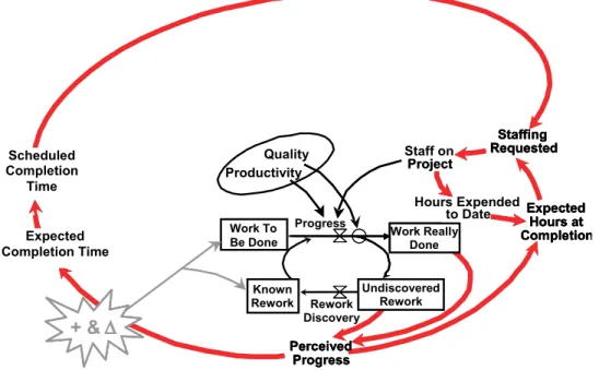
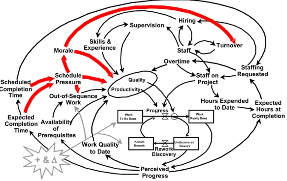
Each of the charts that follows describes the cause-effect relationships that occur on projects and are represented in the model. Each arrow represents a causal relationship as, in the example below, “staffing requested” affects the “staff on project.”

Lower levels of reusability translate to the program as higher amounts of work that must be done. We represent that in Figure 5 with a “+ & ∆” to represent (a) more work to do with less reuse and (b) late and changing information from a precedent program (which does not actually increase workscope directly, but does reduce the productivity with which work is done). The obvious direct consequence of each condition is that estimates of expected hours of work increase. If no accompanying schedule adjustment is made, higher staffing will be required to complete the bigger job in the same time frame.

The requirement for higher staffing levels may have the immediate effect of requiring overtime from current staff, and the mid-term effect of new hiring (Figure 6). The overtime, particularly if at high levels and sustained, will tend both to reduce productivity and to increase error creation. In some cases real output is lost as a result of too much overtime [13]. Hiring is increased by the low reuse scenario relative to the no risk baseline, as new labor is brought in to accomplish the more work in the same schedule. (See Figure 7 for plotted results from these illustrative simulations.) Similarly, when we add the

late information, hiring needs increase. When both

risks are added in together, however, the hiring needs increase by more than the sum of the individual parts. The hiring needs increase higher, and extend longer.

Years People Lines of Code Completed Terrible Productivity ?

?

?

?

?

?

?

Figure 3. After strong early start, progress often falters.

Figure 4. The rework cycle

Rework Discovery

People Productivity Quality Work To

Be Done WorkDone

Undiscovered Rework Known

Rework DiscoveryRework

People Productivity Quality Work To

Be Done WorkDone

Undiscovered Rework Known

The problems caused by one risk interplay with those caused by the other. Note that the program not only becomes more expensive, but it also takes longer. While this paper focuses on cost impacts, clearly these impacts pose schedule risk as well.

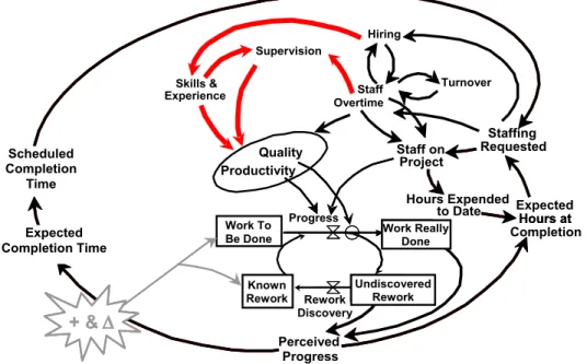
As new staff is hired (particularly in a constrained labor market), skill dilution is likely. Even if the new hires are highly skilled, they will still require

experience on the specifics of this particular software development effort and acclimation to the organization. Further, the supervisors and team leaders will begin to feel stretched as the team size grows. Both effects further degrade both productivity and work quality (Figure 8).

Just as the hiring needs compound, so too does the dilution of workforce skill (see plots in Figure 9). The

Figure 5. Increased workscope drives the need for additional staff.

Staff on Project Quality Productivity Undiscovered Rework Really Done Work Staffing Requested Expected Hours at Completion Hours Expended to Date Perceived Progress

+ &

'

+ &

'

+ &

'

+ &

'

Figure 6. Higher staffing levels require hiring and/or overtime.

Completion Staff on Project Quality Productivity Undiscovered Rework Really Done Work Staffing Requested Expected Hours at Hours Expended to Date Perceived Progress

+ &

'

Progress _{Work Really}

Perceived Progress

+ &

'

+ &

'

Expected

Completion Time Done

50 Base—"as planned" Low Reuse 40 Late Information Both Risks Hiring ₃₀ (People/ Month) 20 10 0 18 2 4 6 8 10 12 14 16 20 22 24

Month from Program Start

Figure 7. Hiring increases dramatically when the two risks are combined.

Figure 8. Hiring drives dilution of supervisory effectiveness and overall team skill levels.

Completion Staff on Project Quality Productivity Undiscovered Rework Really Done Work Staffing Requested Expected Hours at Hours Expended to Date Perceived

+ &

'

+ &

'

+ &

'

+ &

'

Month from Program Start

Both Risks Low Reuse

Late Information

Base—as planned

Figure 9. The impact of reduced skill lingers far longer when the program faces both risks.

resulting effect on productivity extends longer with both risks present, and the effect is deeper than would be indicated by simply adding the two individual impacts.

Consider as well that we depict here the baseline labor market, but the degradation in performance would be worse still were we to “layer in” an additional labor market risk.

Several months down the road, the effect of the earlier rework begins to be evident. Rework that had been created by the new, less experienced staff and the old, more fatigued staff begins to propagate, as subsequent work products incorporate errors from earlier faulty ones (Figure 10).

We can count on there being rework in the late

stages of a program. The magnitude of this rework is instrumental in determining the cost and schedule performance of a program. As illustrated in the Figure 11 plots, the impacts of lower reuse cause a worsening of rework that is exacerbated by the late information

risk.

Later still, the pressures of simultaneously overrunning the budget and schedule, while finding more and more rework, generate staff morale problems, furthering the decline in performance (Figure 12 and 13).

On an ongoing basis, these problems continue to feed back upon themselves, affecting the productivity and quality of work done throughout the program; see plots in Figure 14. Even downstream independent

H ir in g ( Pe op le /M on th )

Month from Program Start

M ul tip lie r o n P ro du ct iv ity o f S ki ll

Figure 10. As work quality suffers from earlier impacts, downstream impacts propagate. Completion Staff on Project Quality Productivity Undiscovered Rework Really Done Work Staffing Requested Expected Hours at Hours Expended to Date Perceived

+ &

'

+ &

'

+ &

'

+ &

'

Months from Program Start

Figure 11. Rework levels reach higher and extend longer with both risks active.

R ew or k ( % o f T ot al W or k)

Month from Program Start

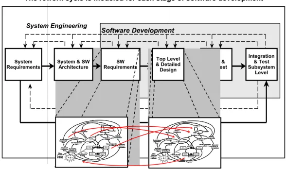
effort that is not directly affected by the risks can be impacted (growing the potential for compounding). As indicated in Figure 15, late and changing upstream work can affect downstream productivity, and delaying downstream progress can slow the discovery of needed rework on upstream products. In these (and other) ways, changes on work that seemed isolated to a particular stage of work can propagate impact on others. Barry Boehm points out the importance of finding and fixing problems early, noting that reworking a requirements problem can cost 50 to 200 times what it would take to fix problems during the requirements phase [14].

How much difference do these risks make in the cost of the program under these different conditions?

Figure 16 (a repeat of Figure 1 at the start of the paper) shows the labor hour impact of combining two individual risks: 10% lower reuse and 2 months late

information. The individual impacts of these two risks

are shown as 13% and 7%, respectively. Combined, the two risks cause a 24% impact, i.e., 20% greater than the sum of the individual risks.

To take the analysis one step further, we have conducted leverage analyses of the risks in combination, looking at varying degrees of magnitude of each risk. (For simplicity, only two risks are repeated; this analysis could encompass any number of risks of interest.) Figure 18 shows the impact on staff costs of both Risk A (less reuse) and Risk B (late information) in combination. In the extreme case of this illustrative analysis, with 20% additional new work from less reuse and information that is five months late, staffing costs soar 80%. How much compounding of risk impacts is this? Figure 18 compares the degree of compounding to the sum of the individual risks. For example, if the sum of the risks is 20%, but together the risks create a 24% impact, the additional four percentage points due to the compounding are a compounding rate of 20% (4/20).

In Figure 18, the zero compounding shown across the 0% lower reuse column and the 0 months late

information row indicate that there is no compounding

when only one risk is present. Once both risks are present, we begin to see compounding—generally more as each of the risks increase in magnitude.

1

0.9

0.8

Multiplier

on Productivity _{Base—as planned} of Morale _0.7 Low Reuse Late Information 0.6 _{Both Risks} 0.5 10 12 14 16 18 20 22 24 2 4 6 8

Months from Program Start

Figure 12. As program performance suffers, the morale of the staff is affected, further worsening matters.

Figure 13. Morale problems compound in the presence of

both risks. Figure 14.extended. Overall productivity problems are worsened and 2 1.75 1.5 1.25 Productivity 1 (KSLOC/ Person/Year) 0.75 Base—as planned 0.5 _{Low Reuse} Late Information 0.25 Both Risks 0 2 4 6 8 10 12 14 16 18 20 22 24

Month from Program Start

Scheduled Completion Time Expected Completion Time Morale Schedule Pressure Out-of-Sequence Work Skills & Experience Overtime Hiring Turnover Staff on Project Staffing Requested Expected Hours at Completion Hours Expended to Date Availability of Prerequisites Work Quality to Date Perceived Progress Quality Productivity Progress Staff Undiscovered Rework Known Rework Work Really Done Work To Be Done Rework Discovery Supervision

+ &

'

Month from Program Start

Pr od uc tiv ity ( K SL O C /Pe rs on /Y ea r)

Figure 15. The same dynamics occur in each program work phase, and the phases interact with one another.

development

System Engineering _{Software Development}

Code & Unit Test Integration & Test Subsystem Level Morale Scheduled Completion Time Expected Completion Time Schedule Pressure Out-of-Sequence Work Skills & Experience Overtime Hiring Turnover Staff on Project Staffing Requested Expected Hours at Completion Hours Expended to Date Availability & Quality of Prerequisites Work Quality to Date Perceived Progress Quality Productivity Progress Staff UndiscoveredRework Known Rework Work Really Done Work To Be Done Rework Discovery + & D Other Phases Progress & Quality Morale Scheduled Completion Time Expected Completion Time Schedule Pressure Out-of-Sequence Work Skills & Experience Overtime Hiring Turnover Staff on Project Staffing Requested Expected Hours at Completion Hours Expended to Date Availability & Quality of Prerequisites Work Quality to Date Perceived Progress Quality Productivity Progress Staff UndiscoveredRework Known Rework Work Really Done Work To Be Done Rework Discovery + & D + & D + & D Other Phases Progress & Quality System & SW Architecture System Requirements Morale Scheduled Completion Time Expected Completion Time Schedule Pressure Out-of-Sequence Work Skills & Experience Overtime Hiring Turnover Staff on Project Staffing Requested Expected Hours at Completion Hours Expended to Date Availability & Quality of Prerequisites Work Quality to Date Perceived Progress Quality Productivity Progress Staff Undiscovered Rework Known Rework Work Really Done Work To Be Done Rework Discovery + & D Other Phases Progress & Quality Morale Scheduled Completion Time Expected Completion Time Schedule Pressure Out-of-Sequence Work Skills & Experience Overtime Hiring Turnover Staff on Project Staffing Requested Expected Hours at Completion Hours Expended to Date Availability & Quality of Prerequisites Work Quality to Date Perceived Progress Quality Productivity Progress Staff Undiscovered Rework Known Rework Work Really Done Work To Be Done Rework Discovery + & D + & D + & D Other Phases Progress & Quality Top Level & Detailed Design SW Requirements

The rework cycle is modeled for each stage of software development

Figure 16. Combined risks generate 20% additional compounded impact (a repeat of Figure 1).

Combined risks generate 20% additional compounded risk

0% 5% 10% 15% 20% 25% 30% Risk A: 5% more scope from less

reusability

Risk B: Late

Information Combined RisksA&B

Percent Labor Month Impact

Risk A Risk B Additional Total Impact When Combined

Pe rc en t L ab or M on th I m pa ct

Figure 17. Combining risks generates compounding cost growth.

Figure 18. As risks grow in magnitude, the degree of compounding increases. 0 _{1 2} 3 ₄ 5 05 1015 20 0 10 20 30 40 50 60 70 80 90 Percent Staffing Growth (%)

Months Information is Late

Lower Reuse Pe rc en t S ta ffi ng G ro w th ( % )

Months Information I_{s Late} Lowe r Reu se 0 ₁ 2 ₃ 4 ₅ 0 510 1520 0 5 10 15 20 25 30 35 40 Compounding %

Months Information is Late

Lower Reuse C om po un di ng %

Months Information I_{s Late} Lowe r Reu

4. Summary

Are there compounding impacts of multiple risks on a program? Can we rely on the adequacy of impact estimates

of each individual risk element in isolation? There is a

strong logical and analytical case for the existence of compounding impacts of multiple risks, and most program managers have experienced it. The analyses illustrated here and conducted on several programs identify it, yet the magnitude of the compounding is situation-dependent and risk-dependent. Indeed, the variation of multiple-risk impact may even include “negative compounding” 4 _{if there are concurrent} effects that offset one another. Regardless of the actual magnitude of the compounding phenomena, impact estimates of individual risk elements clearly may not be adequate when made in isolation of other risks. Additional research and analysis is to be done in order to understand typical patterns of compounding impacts, even to develop heuristics for future estimating. Most importantly, more research and education is needed in order to improve understanding of the nature and causation of compounding impacts. Only with that improved understanding will we be better able to design and implement informed program plans and effective mitigating management actions.

5. References

[1] GAO Report Number 05-301, Defense Acquisitions: Assessments of Selected Major Weapon Programs, March 2005.

[2] Cooper, Kenneth G. “Toward a Unifying Theory for

Compounding and Cumulative Impacts of Project Risks and Changes,” PMI, 2004.

[3] Pinto, Jeffrey, and Peter Morris, eds. “Project Changes: Sources,

Impacts, Mitigation, Pricing, Litigation & Excellence,” In The Wiley Guide to Managing Projects, Hoboken, NJ: John Wiley & Sons, Inc., 2004

[4] Lyneis, James M., Kimberly Sklar Reichelt, and Carl G. Bespolka. “Calibration Statistics for Life-Cycle Models.” In Proceedings of the 1996 System Dynamics Conference, 1996. [5] Stephens, Craig A., Alan K. Graham, and James L. Lyneis.

“System Dynamics Modeling in the Legal Arena: Special Challenges of the Expert Witness Role,” In Proceedings of the 2002 System Dynamics Conference, 2002.

[6] Cooper, Kenneth G. “Naval Ship Production: A Claim Settled

and a Framework Built,” Interfaces 10(6, 1980): 30–36.

[7] Abdel-Hamid, Tarek, and Stuart E. Madnick. “Lessons Learned from Modeling the Dynamics of Software Development,”

Communications of the ACM 32 (12, December 1989): 1426– 1438.

[8] Eden, Colin, Terry Williams, Fran Ackermann, and Susan Howick. “On the Nature of Disruption and Delay (D&D)

in Major Projects,” Journal of the Operational Research Society

51(3): 291–300.

[9] Mechanical Contractors Association of America. “Change Orders, Overtime and Productivity,” Publication M3, Rockville, MD, 1994.

[10] Adrian, Jim. “The Impact of Temperature on Productivity,”

Construction Productivity Newsletter 19(5).

[11] Ibbs, C. W., and Walter E. Allen. “Quantitative Impacts of

Project Change,” Source Document 108, Construction

Industry Institute, Austin, TX, 1995.

[12] Jones, Capers. Applied Software Measurement, McGraw-Hill Computing, 1996.

[13] Cooper, Kenneth G. “The $2000 Hour: How Managers

Influence Project Performance Through the Rework Cycle,”

Project Management Journal 25(March 1994).

[14] Boehm, Barry, and Philip N. Papacccio. “Understanding and

Controlling Software Costs,” IEEE Transactions on Software

Engineering 14(10, October 1988): 1462–1477.

Author Biographies

Sharon A. Els has been a consultant specializing in

system dynamics simulation for over fifteen years. She

is a Managing Consultant in PA’s Federal and Defense Services practice. Her client work has included: optimizing corporate resource allocation, predicting market changes and evolution, delivering projects on time and on budget, and resolving large contract disputes. She has authored numerous articles on using dynamic models for program management analysis. She holds a Bachelor’s degree in civil engineering from MIT, and an MBA from MIT’s Sloan School.

Kimberly Sklar Reichelt is a consultant with PA’s Federal and Defense Services practice. She has been designing and building simulation models for use in consulting assignments for nearly twenty years. These assignments have ranged from business strategy to litigation support, from issue-mapping and scenario-planning workshops to developing analytical model-based comprehensive analyses. Prior to joining PA, Kim received both her Bachelor’s and Master’s degree in management science from MIT’s Sloan School of Management.

Kenneth G. Cooper’s management consulting

career spans thirty years, pioneering the field of project

management simulation and the application of computer simulation models to a variety of other strategic business issues. Mr. Cooper is an original author of the simulation models used in conducting the analyses reported herein, and has published extensively on the topic of project management, rework, change impacts, productivity conditions, and performance improvement. He is Managing Director of Cooper Associates, Milford, NH.

4. Is there such a thing as negative compounding? Yes, sometimes two risks in combination can create cost and/or schedule savings for a program. For example, one of our clients was faced with

significant added work to do, which normally would have forced them to increase staff considerably to achieve the planned schedule milestones. This extra staffing and overtime may have set off all the negative dynamics of rapid hiring, extra overtime, compromised quality and staff fatigue. However, at the same

time, a critical technical component was delayed forcing a “non-negotiable” schedule slip. In this case, labor hours were saved, but of course they did not meet the original milestones because of the delayed technical component.