THE CHARACTER OF PLANAR TESSELLATIONS WHICH ARE NOT SIDE-TO-SIDE

THE CHARACTER OF PLANAR TESSELLATIONS WHICH ARE NOT

SIDE-TO-SIDE

R

C

C

T

¨

B,

1_{School of Mathematics and Statistics, University of Sydney, NSW 2006, Australia;}2_{Faculty of Mathematics,} Ruhr-University Bochum, Germany

e-mail: rcowan@usyd.edu.au, cthaele@uos.de

(Received July 23, 2013; revised December 3, 2013; accepted December 15, 2013)

ABSTRACT

This paper studies stationary tessellations and tilings of the plane in which all cells are convex polygons. The focus is on the class of tessellations which are not side-to-side. The character of these tessellations is explored, with special attention paid to the relationship between edgesof the tessellation and sidesof the polygonal cells and to the combinatorial topology between the ‘adjacent’ geometric elements of the tessellation. Three new parameters,ε0,ε1andε2summing to unity, are introduced. These capture the essence of non side-to-side

tessellations and play a role in understanding the adjacency of sides and cells. Examples illustrate the theory. Keywords: combinatorial topology, Delaunay tessellation, random tessellations, STIT tessellation, stochastic geometry, tilings.

INTRODUCTION

As discussed in the recent paper of

Weiss and Cowan (2011), the focus of attention in most studies of planar tessellations and tilings has been the side-to-side case, where each side of a polygonal cell coincides with a neighbouring cell’s side. The studies ofCowan(1978;1979) are early exceptions in the random tessellation theory. Those studies, which also have relevance to the tiling literature, introduced a new parameter φ. It quantified one of the most important features of non side-to-side tessellations, namely the occurrence of a type of vertex not seen in the simpler side-to-side case: the so-called π-vertex. If a vertex has j emanating edges, there are j angles subtended by these edges at the vertex. If one of these angles is equal toπ, the vertex is called aπ-vertex. A vertex that is not aπ-vertex is called aπ−-vertex. The parameter φ is defined as the proportion of vertices which areπ-vertices.

Many properties of a non side-to-side tessellation can be expressed in terms of φ together with another parameter,θ, the mean number of emanating edges from the typical vertex. These fundamental parameters, which capture both topological and combinatorial aspects, satisfy the general constraints

0_≤φ_≤1 ; 3_≤θ_≤6₋2φ, (1)

as proved in Weiss and Cowan (2011) and illustrated in Fig. 5a. There are, however, some entities of a combinatorial and/or topological nature which cannot be expressed as a function ofθandφ. So it is clear that

other parameters of the non side-to-side tessellation are important. In this paper, we investigate these issues, delving into some of the finer structure of tessellations which are not side-to-side. Some metric issues are also discussed and one parameter, the mean length of the typical tessellation edge, plays a prominent role.

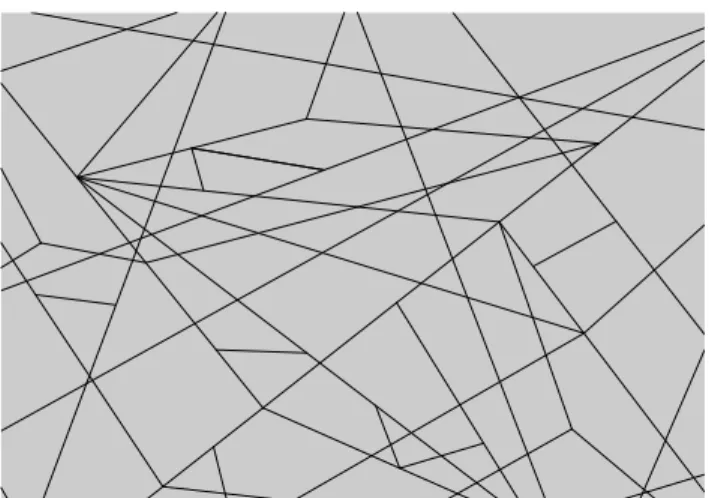
Fig.1illustrates that a general random tessellation allows any shape or size of convex polygon to be a cell; furthermore it potentially allows any number and geometry of edges emanating from a tessellation vertex. Some models, however, might restrict the variation of these features somewhat.

GEOMETRIC OBJECTS AND

THEIR ADJACENCY

A tessellation of the plane is a collection of compact convex polygonalcellswhich cover the plane and overlap only on their boundaries. The union of the cell boundaries is called the tessellation frame. Each cell hassidesandcorners, these being respectively the 1-faces and 0-faces of the polygon, which lie on the frame. The union (taken over all cells) of the cell’s corners is a collection of points in the plane called the verticesof the tessellation. Those line segments which are contained in the frame, have a vertex at each end and no vertices in their interior are callededgesof the tessellation.

Two cells are said to be equal under motion if one can be found by translating and/or rotating the other. A tiling is a tessellation with a finite number of equivalence classes under this ‘motion’ relationship. Often a tiling seen in the literature has no randomness, but we also permit tilings generated randomly. Most tilings use only a small number of polygons with congruent copies of these assembled to cover the plane.

Our random planar tessellations (or planar tilings) are assumed to be stationary – and also locally-finite (avoiding points and line-segments ‘accumulating’).

The stationarity condition says that the geometric features are statistically invariant under translation. To achieve this with a non-random tiling, such as in Fig.6, one must ensure that the planar origin is uniformly distributed in the repeating sub-unit. Hybrid models (partly random, partly non-random) can arise too, for example in the 2_×1 tiling example in a later section; in that case, stationarity is created if the origin is uniformly distributed inside one of the original 2_×2 squares.

The tessellation’s primitive geometric elements, treated as compact domains, are the vertices, edges and cells. The sets of these elements are denoted by V, E and Z (for Zellen) respectively. These are the tessellation elements studied in the standard texts (Stoyanet al., 1995; Schneider and Weil, 2008). In this paper, however, other compact geometric elements will be introduced and the set of these will also be denoted by an upper–case letter – for example, the sets SandCof allsidesandcornersof cells, respectively.

We note that, for those elements which are not primitive but are instead derived from a primitive element, then the set may indeed be a multi-set. For example, in side-to-side tessellations, everys_∈S equals another member ofS, as befits the terminology

side-to-side. This may be true for some (but not all) members ofSin the non side-to-side case.

Generic sets of compact geometric objects are denoted byX andY. Subsets of the setX are denoted by X[_·], with the contents of the [_·] being a suitably suggestive symbol introduced in anad hocmanner. For example, we denote the sub-class ofπ-vertices byV[π]

and the subclass of−π-vertices byV[π−].

Point processes and their intensities: The centroids of all members in a set of objects form a stationary point process on the plane, but this process might also have point multiplicity and, if so, it would not be asimplepoint process.

DEFINITION1:The intensity of objects belonging to class X is the intensity of the point process inR2 formed by centroids of the elements of X . It is denoted byλX.

The scale of the tessellation is determined by one of the intensity parameters and we have chosen λV to play this scaling role. Our locally-finite condition implies that λV is finite. The other main intensities, reported inWeiss and Cowan(2011), are expressed as follows in terms ofλV and are also finite:

λE=

θ

2λV, λZ=

θ₋2

2 λV, λS= (θ−φ)λV, (2)

withλC=λS. From these identities, we have

λS=

2(θ₋φ)

θ λE , (3)

showing clearly the way this changes fromλS=2λE as we move away from the side-to-side case which has

φ=0.

Metric parameters: There are many classes of line-segment that can be defined in a tessellation. The lengths of these segments together with the perimeters and areas of cells are the most obvious metric properties relevant to our study. The following notation applies.

DEFINITION 2:If the class X comprises elements which are line-segments, we letℓX be the mean length of these segments. In particular,ℓ¯Eandℓ¯Sare the mean edge length and mean side length respectively. We let

¯

ℓZbe the mean cell perimeter anda¯Zbe the mean cell area.

It is known, fromCowan(1978), that ¯aZ=1/λZ= 2/(λV(θ−2))so ¯aZ is not a new parameter. The other metric entities ¯ℓE,ℓ¯S and ¯ℓZ are related to the frame intensity. The frameY _{of the tessellation is the union}

unit area. The text ofStoyanet al.(1995) shows that theframe intensityequals bothλEℓ¯E and 1₂λZℓ¯Z, so

¯

ℓZ=2

λE

λZ ¯

ℓE= 2θ

θ₋2ℓ¯E , (4)

to which we addframe intensity= 1₂λSℓ¯Sand the new formula

¯

ℓS=2

λE

λS ¯

ℓE =

θ

θ₋φℓ¯E. (5)

We see in Eq.5how the mean side length ¯ℓS departs from equality with the mean edge length ¯ℓE as φ becomes positive (that is, as the tessellation departs from the side-to-side case). These metric entities are inter-related; in this paper we have chosen ¯ℓE as the principal metric parameter.

Window formulae and transects: Other properties of the tessellation observed in a window W, chosen without reference to the tessellation itself, are known (see formula (3.4) in Cowan, 1978). The most interesting of these are for convexW when the tessellation processY _{is assumed isotropic (that is, its}

geometric features are statistically invariant under any planar rotation). In this case, the number of edges of the tessellation intersectingW has expectation

EKW(E) =ℓ¯E

π Perim(W) +Area(W)

λE. (6)

Here we use the notationKW(X), defined as the count ofX-type objects intersectingW. Also the number of cells intersectingW has expectation

EKW(Z) =1+

ℓ¯_E

π Perim(W) + θ₋2

θ Area(W)

λE . (7)

To these we now add the expected number of the tessellation’s line-segments of a given classX which intersectW:

EKW(X) =ℓX

π Perim(W) +Area(W)

λX , (8)

as shown by formula (6) ofCowan(1979), a paper that deals with general isotropic line-segment processes.

When W is a line-segment, of length ℓ say, then each of the window formulae simplify, because Area(W) =0 and Perim(W) =2ℓ.

REMARK 1: With such a W and letting ℓ_→∞, Eq. 6 indicates informally that the point process formed by the intersection of tessellation edges with a line transect (chosen without reference to the tessellation) has intensity 2 ¯ℓEλE/π. In some

tessellation models, the point process on this transect is a Poisson process and then the number KW(E) of edges hitting a line-segment W of length ℓ has the property

P{KW(E) =k_|ℓ_}=(ρℓ)

k_e−ρℓ k! ,

where

ρ= 2

πℓ¯EλE.

In these ‘Poisson Transect models’, the Buffon-Laplace problem is effectively solved, giving a chance e−ρℓ that a needle of length ℓ thrown randomly onto the tessellation Y _{lies wholly within a cell of the}

tessellation. To understand this assertion, note that the thrown needle W is assumed to be an isotropic random set. Eqs. 6–8, with expectations taken of the perimeter and area of W , are valid when W is an isotropic random set even ifY _{is not isotropic.}

Adjacency: The standard texts (Stoyanet al., 1995; Schneider and Weil, 2008) discuss only the primitive elements V,E and Z. Their notation which works well in that restricted context is unsuitable when other object classes like S orC are introduced, because then object classes are not uniquely defined by their dimension. For example, the textbook notation

λ1 used for the intensity of edges E (because edge have dimension one) cannot be used when there is another object class, sidesS, whose elements also have dimension one. This notational deficiency becomes serious for tessellations in R3 (Weiss and Cowan, 2011) but, even in _R2, we find advantage in adopting the notation used in Weiss and Cowan (2011). We recommend to the reader the first two sections of their paper, as it provides further discussion and motivation for the notation.

DEFINITION 3: An object x _∈ X is said to be adjacent toan object y_∈Y if either x_⊆y or y_⊆x. For any x_∈X , the number of objects of type Y adjacent to x is denoted by mY(x). For a random tessellation we define µXY as the expected value of mY(x) when x is the typical member of X . Formally, we write

µXY := EX(mY(x)), where the symbol EX (and the probability measurePX on which it is based) indicate that we are dealing with the typical element of type X (Stoyan et al.,1995; Weiss and Cowan, 2011). The second moment EX(mY(x)2) of the number of type Y objects adjacent to the typical X object is written as

µ_XY(2).

the quantities expressible solely in terms of θ and φ

(Weiss and Cowan,2011):

µSE=

θ

θ₋φ, (9)

which clearly equals 1 in the side-to-side case.

The nine values of µXY where both X andY are primitive elements, that isX andY _{∈ {}V,E,Z_}, can all be expressed solely in terms ofθ(Stoyanet al.,1995; Weiss and Cowan,2011). The most important two can be presented as follows.

µZE=µZV = 2θ

θ₋2, (10)

which were first proven for the general case inCowan (1978;1980) andMecke(1980), though they had been mentioned without proof and in restricted cases earlier. In the side-to-side case, the right-hand side of Eq. 10 also equals the expected number of sides (or corners) of a typical cell – but these entities take a different form in the non side-to-side case, as we discuss in a later subsection.

WhenX andY are both primitive-element classes, it has been shown inMecke (1980),Weiss and Z¨ahle (1988) andLeistritz and Z¨ahle(1992) that

λXµXY=λYµY X, (11)

and this identity also holds when eitherX orY or both are classes offaces of primitives; Møller’s Theorem 5.1 (Møller,1989) provides the proof of this extension. As an example,

µSE=

µESλE

λS

= θ

θ₋φ,

proving Eq. 9 with the use of Eq. 3 and the obvious factµES=2.

In concluding this subsection, we note thatθ and

φ can be expressed using the adjacency notation;

θ = µV E and φ = µ_{V S}◦, the expected number of ‘side-interiors’ adjacent to a typical vertex (where the interior of a side, or indeed of any object x of lower dimension than the space of the tessellation, is defined using the relative topologyon x). Also ˚X denotes the class comprising the relative interiors of objects in classX. For brevity we drop the word ‘relative’ in the sequel; ‘interior’ means ‘relative interior’.

Faces ‘owned by’ other objects: As proved in Cowan (1978; 1980) and used in applications (Cowan and Morris,1988;Cowan and Tsang,1994),

ν1(Z) =ν0(Z) =

2(θ₋φ)

θ₋2 , (12)

whereν1(Z)andν0(Z) are the mean number of sides and corners of the typical cell. This is an ownership concept rather than anadjacency; not all sides that are adjacent to a cell belong to it. Theνnotation in Eq.12 will be generically defined shortly in Definition 4, after we discuss an application.

Eq. 12 has application to the type of question common in the literature on tilings. “Can we tile the plane using only convex pentagonal tiles?”. Obviously we can, there being examples using congruent copies of some particular pentagons (Gr¨unbaum and Shephard, 1987). But Eq. 12, combined with Eq. 1, tells us that we certainly can’t do so if φ > 1₂, even if we use convex pentagons of differing sizes and shapes (because then θ would be

<3). The bounding case, with φ = 1₂ and θ = 3, can be realised so easily – start with the hexagonal lattice (made stationary in R2 by placing the origin uniformly distributed within a hexagon) and divide every hexagon into two pentagons with a chord, ensuring that chord-ends never meet – that we might expect higherφvalues are possible. But they are not!

DEFINITION 4: Let X be a class of convex polytopes, all members of which have dimension i. For j < i, we define nj(x) as the number of j-faces of a particular object x_∈X . Define νj(X) :=

EX(nj(x)), the expected number for the typical X -object. We define Xj,j<i, as the class of objects which are j-dimensional faces ( j–faces) of some polytope belonging to X .

We shall use this notation in the planar case mainly when j=0 and i=1. For example, E0 is the class of edge-termini andS0the class of side-termini. Also Z0 and Z1 are the classes of cell corners and sides respectively; also known by the labelsC andS which we retain for convenience, except when defining the important entities,ν1(Z)andν0(Z).

The disparity between the number of edges adjacent to a cell z (that is, on the boundary of z) and the number of sides owned byzprovides another measure of departure from the side-to-side status. This suggested measure isµZE−ν1(Z)which, from Eq.10 and Eq.12, equals 2φ/(θ₋2). This measure which we call thecell boundary disparitylies in the range[0,2]; the upper bound occurs in a number of models, notably in the STIT model which we discuss later in the paper.

OTHER PARAMETERS AND THE

EQUALITY

_RELATIONSHIP

another type of element. Consider µCE, the expected number of edges adjacent to a typical cell corner. The typical sampling of the corner gives a number-of-edges-emanating bias to the sampling of a vertex, and this leads to the introduction into the formula of µV E(2), the second moment of the ‘number of

edges emanating from the typical vertex’. As shown inWeiss and Cowan(2011),

µCE=

µ_{V E(2)−}φ µ_V[π]E

θ₋φ , if φ>0, (13)

whilstµCE=µV E(2)/θifφ=0. Eq.13also introduces µV[π]E, the expectation of the number edges emanating from the typicalπ-vertex, an entity defined whenφ>

0. For brevity, we denote it by θπ; we also use θ−

π for µ

V[−π]E, though this is not another new parameter because

θ_≡µV E=φ µV[π]E+ (1−φ)µ_V[−

π]E ≡φ θπ+ (1−φ)θ−

π . (14) REMARK2: Interestingly, whilst we see in Eq.1that

θ (which _≡µV E) is bounded above, examples show thatθπ andθ−

π can be arbitrarily large. For example, it is easy to construct a tessellation with very fewπ -vertices with each π-vertex having n edges, n being arbitrarily large. Another example is available, with non-π vertices being rare but emitting n edges, where n is large (details omitted).

Weiss and Cowan (2011) have used the four parameters (θ and φ, together with the additional parameters, µ_{V E(2)} and θπ) to give formulae for all relevant intensity parametersλX and for all but three of the forty-nine µXY entities between the seven classes of elements that they study: X and Y both ∈ {E,V,Z,E0,C,S,S0_}. This suggests that three more parameters are required, and we could choose to use the three missing entries inWeiss and Cowan(2011),

µSZ,µZSandµSS– but actually two suffice becauseµSZ and µZS are related (via Eq. 11). There are however more natural choices, as we shall see later in this section.

The equality relationship: The relationship between edge and side, and the cell ‘owning’ the side, will occupy much of our attention in this paper. The complications in their adjacency relationship is demonstrated in Fig. 2, perhaps explaining why formulae for the missing trio have not yet been found for the general non side-to-side tessellation, nor for any model until recently.

In the side-to-side case,mS(e) =2 for everye_∈E. Despite the added complication seen in Fig. 2 which

arises in the non side-to-side case, this identity still holds – because adjacency involves thesubsetconcept; every e_∈ E is a subset (_⊆) of two sides. To better capture how edges and sides relate, we need to focus on another relationship,equality.

DEFINITION 5: Suppose the objects in class X have the same dimension as those in class Y . Then the number of objects of type Y equal(as a set inR2) to some x_∈X is denoted by the random variable mY(x). We defineµ_XY asEX(mY(x)).

It is the loss ofequalityofEandS, rather than their loss of adjacency, that happens when a tessellation is not side-to-side. An edge is not always equal to the side of two cells, that is, mS(e),e_∈ E may not always equal two; it takes the values 0,1 or 2 randomly. Depending on this value, the class E can be divided into sub-classesE[0],E[1]andE[2].

mS(s) =2

mS(s) =2

mE(s) =1

mE(s) =1

mS(s) =5

mE(s) =4

mE(s) =4

mE(s) =4

mS(s) =4

mE(s) =2

mS(s) =3

mS(s) =1

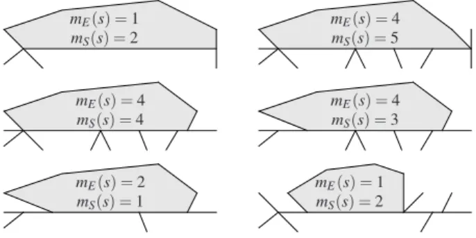
Fig. 2.The shaded region is a cell; one of its sides is the horizontal line-segment which bounds it below. This side s has a varying number mE(s)of edges contained within it, as shown. The value of mS(s), the number of sides adjacent to it (the count including s itself), also varies as shown.

We introduce, for the typical edge, the probabilities

ε0,ε1andε2 for these three outcomes. Naturally,ε0+

ε1+ε2=1, and

µ_ES=ε1+2ε2. (15)

When needed, we use symbols ¯ℓE[0],ℓ¯E[1] and ¯ℓE[2]for

the expected lengths of typical edges of the three sub-classes; obviously,ε0ℓ¯E[0]+ε1ℓ¯E[1]+ε2ℓ¯E[2]=ℓ¯E.

We now consider the random variablemE(S), the number of edges equal to a typical side. It is binary, taking only the values in _{0,1_}. So, using Eq. 3 and Eq.15,

PS{mE(s) =1_}=µ_SE

=λE

λS

µ_ES= θ(ε1+2ε2)

Also used in this expression is the analogue of Eq.11; such analogues exist for all symmetric relations.

Another descriptor of ‘not being side-to-side’ is

µ_SS, the expected number of sides equal to a typical side. This is derived as follows:

µ_SS=1+µ_SE[2]=1+

2λ_E[2] λS

=1+ ε2θ

θ₋φ, (17)

usingµ_E[2]S=2 and Eq.11.

The missing mean adjacencies in terms of the epsilons: We now show that the three missing mean adjacencies, µSZ,µZS and µSS, can be expressed in terms ofθ,φ,ε0,ε1andε2.

THEOREM 1: The three mean adjacencies

missing in the table of forty-nine such entities in

Weiss and Cowan(2011) are

µSZ=1+

θ(ε1+2ε2)

2(θ₋φ) , (18)

µZS=

2(θ₋φ) +θ(ε1+2ε2)

θ₋2 , and (19)

µSS=1+

θ

θ₋φ(1−ε0). (20)

PROOF: Note thatmZ(s) =1+mE(s),for alls∈S, so µSZ = 1+µSE and Eq. 18 follows by applying Eq. 16. Furthermore, via Eq. 11, µZS = λSµSZ/λZ and this equals Eq. 19 using λZ = 1₂(θ−2)λV and

λS= (θ−φ)λV.

To prove Eq.20, we start with a subtle expression formS(s), the number of sides adjacent to a particular sides(see Definition 3). For all sidess,

mS(s) =1+mE(s)₋mE[0](s). (21)

The proof of this is essentially given by the diagrams in Fig. 2, treating the horizontal line-segment that bounds the shaded cell below as our particulars. Essentially, the six diagrams present all of the complexity that a neighbourhood ofsmight have. It readily follows from Eq.21that

µSS=1+µSE−µSE[0]

=1+λE

λS

µES−

λ_E[0] λS

µ_E[0]S using Eq.11

=1+λE

λS

µES−

λE[0] λE

λE

λS

µ_E[0]S

=1+2λE

λS

1₋ε0

=1+ θ

θ₋φ(1−ε0),

using the definition ofε0, the fact thatµES=µE[0]S=2 and Eq.3. Therefore, identity Eq.20has been proved

and the theorem’s proof is complete.

We consider thatε0,ε1 andε2capture the essence of ‘not being side-to-side’, and so we adopt them as fundamental parameters instead of µSZ,µZS and µSS, which are not as immediately relevant to the concept of side-to-side. Thus thetopologicalparameter set of our choice now becomes_{θ,φ,µ_{V E(2)},θπ,ε0,ε1,ε2}, with

ε0+ε1+ε2=1. Our scale parameterλV has relevance too, but it doesn’t influence the combinatorial topology of our system. Nor does our main metric parameter ¯ℓE have topological relevance.

EXAMPLES

A 2_×1 tiling: As a relatively simple learning example, consider the square lattice made up of 2_×2 squares. Each square is then tiled by two 2_×1 tiles, with random orientation for the long axis of these two tiles (vertical or horizontal with equal probability). The bold lines in Fig.7illustrate the construction. Find all the parameters of the tessellation — to reinforce the notation and the relationships between the parameters!

Looking at the typical cell, clearly ¯aZ=2, ¯ℓZ=6 and ν1(Z) =4. Therefore λZ =1/a¯Z = 1₂ and, from Eq. 12, φ =4₋θ. Note also that µZV = 9₂, because on one side (and only one) of each tile there is an extra vertex added with probability 1₂. Therefore, from Eq. 10, θ = 18₅. Then φ =4₋θ = 2₅. Now we can write λV =2λZ/(θ−2) = 58 and λE =θ λV/2= 98, using Eq.2. Also writeλ_V[π]=φ λV =14. It is obvious that ε0 =0 and that λE[1] = 2λV[π] = 12. Therefore

ε1=λE[1]/λE = 4₉, ε2=1−ε0−ε1= 5₉ and λE[2]= ε2λE=5₈. The line intensity is ₂1ℓ¯ZλZ, which equals3₂; the line intensity is also ¯ℓEλE, so ¯ℓE =4₃. As obviously

¯

ℓ_E[1]=1, we derive ¯ℓE[2]= (ℓ¯E−ℓ¯E[1]λE[1])/λE[2]=43. Finallyθπ=3 andµV E(2)=9φ+16(1−φ) = 665.

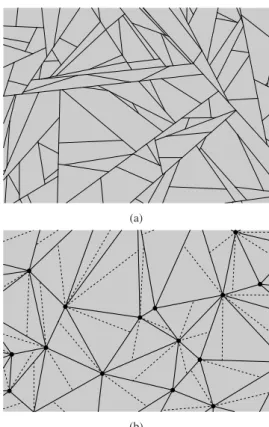
The STIT model: This tessellation, perhaps the best-known model that is not side-to-side, was first studied by Nagel and Weiss (2003; 2005), and later by them in collaboration with Mecke (Meckeet al., 2007;2011). Other recent studies of the planar STIT tessellation are by Schreiber and Th¨ale (2010; 2013) and Cowan (2013). In this model, drawn in Fig. 3a, all vertices areπ-vertices with three edges emanating, soθ _≡µV E =θπ =3,µV E(2)=9 and φ =1.

Forty-six adjacency entities can now be evaluated from Weiss and Cowan (2011), the most interesting in the context of the current paper being µSE = θ/(θ−

φ) = 3

importantν entity, the mean number of sides for the typical cell:

ν1(Z) =

2(θ₋φ)

θ₋2 =4.

So thecell boundary disparityis 2.

The results given above for the STIT model are not new (see Nagel and Weiss, 2005), but, until the recent paper (Cowan, 2013), STIT results for ε0,ε1,ε2,ℓ¯E[0],ℓ¯E[1],ℓ¯E[2],µSZ,µZS and µSS were unknown. From this recent paper, we state the following values:

ε0= 2₃(2 log 2−1) ≈0.25753,

ε1= 2₃(5−6 log 2) ≈0.56075,

ε2= 1₃(8 log 2−5) ≈0.18173,

¯

ℓ_E[0]= 3(3−4 log 2)

2(2 log 2₋1)ℓ¯E ≈0.883 ¯ℓE,

¯

ℓ_E[1]=

3(8 log 2₋5)

2(5₋6 log 2)ℓ¯E ≈0.972 ¯ℓE,

¯

ℓ_E[2]=

3(3₋4 log 2)

8 log 2₋5 ℓ¯E ≈1.251 ¯ℓE.

Here, ¯ℓE = 1₃

p

2π/λV. From these values, together with Eqs.15–19 from the current paper, we have the following results:

µ_ES=ε1+2ε2=4₃log 2≈0.9242,

µ_SE=PS{mE(s) =1}=log 2≈0.6931,

µ_SS=1+ ε2θ

θ₋φ =4 log 2−

3

2≈1.2726,

µSZ=1+log 2≈1.6931,

µZS=4+4₃log 2≈4.9242.

Also derived inCowan(2013) is

µSS= 7

2−2 log 2≈2.1137,

together with full distributions for many of the STIT adjacency relationships. It is readily seen that µSS calculated by the new formula, Eq.20 in Theorem 1, agrees with the result inCowan(2013).

Divided Delaunay: Start with a stationary and isotropic Delaunay tessellation D_{0 based on a}

planar Poisson point process with intensity ρ (the dots in Fig. 3b). This tessellation is illustrated by the solid line segments in the figure, connecting ‘neighbouring’ Poisson dots (see the formal definition in Schneider and Weil (2008)). This tessellation is side-to-side, so has φ = 0. Also, since all cells

are triangles, ν1(Z) =3 and therefore θ =6 from Eq.12. The second moment,µ_{V E(}2), introduced above,

is known in the form of a complicated multiple integral which evaluates to be 37.7808 approximately (Heinrich and Muche,2008). ObviouslyλV =ρ; then using Eq.2we getλE =1₂θ λV =3ρ andλZ=1₂(θ− 2)λV =2ρ. Also, becauseλE[2] =λE, it is clear that

ε2=1. Note that ¯ℓE =32/(9π√ρ)(Miles,1970).

(a)

(b)

Fig. 3. (a) A realisation of the STIT model within a rectangular viewing window. (b) The ’divided Delaunay’ model. The chords are shown as dashed lines.

In each ofD_{0’s triangular cells we independently}

choose a vertex (each equiprobable) and construct a chord from that vertex to a uniformly distributed point on the opposite side of the triangle (see the dotted line segments in Fig. 3b). We label the new tessellation

D_{1. Further iteration using the same random division}

rules yields D_2,D_{3, ..., each being a tessellation with}

only triangular cells. Using superscripts (n) for the parameters of D_{n (even when n=0), we note that if}

n_≥1,

λ_Z(n)=2λ_Z(n−1), λ_V(n_[π)_]=λ_Z(n−1)+λ_V(n_[π−_]1),

λ_E(n)=2λ_Z(n−1)+λ_E(n−1), λ_V(n)=λ_Z(n−1)+λ_V(n−1),

θ(n)=6₋2φ(n),

cells). These four difference equations are readily solved to give

λ_Z(n)=2n+1ρ, λ_E(n)= (2n+2₋1)ρ,

λ_V(n)= (2n+1₋1)ρ, λ_V(n_[π)_]=2(2n₋1)ρ,

and these solutions yield a formula forφ(n)_{which leads}

toθ(n)_:

φ(n)= λ

(n)

V[π]

λ_V(n) =

2(2n₋1)

2n+1₋₁

=_⇒ θ(n)_{= 6}

−2φ(n)₌₂2n+2−1

2n+1₋₁ .

Thus thecell boundary disparityis 1₋2−n, which rises from zero to a limit of 1 asnincreases.

So for D_{1, λ}(1)

V =3ρ, λ

(1)

E =7ρ, φ(1)= 2 3 and

θ(1)₌ 14

3. Also forD1the calculation of the epsilons is easy because D_{0 is side-to-side and therefore has}

only E[2] edges. An edge from D_{0 is divided into}

three segments with probability 1/9, into two segments with probability 4/9 and remains unchanged with probability 4/9. Thusλ_E(1_[2)_] =λ_Z(0)+1_·4₉λ_E(0_[2)_]= 10₃ρ, after allowing for the unchanged edges which remain as typeE[2]. Furthermore,λ_E(1_[0)_]=1₉λ_E(0)= 1₃ρ, as one type-E[0]edge arises when an original edge is hit by two chords. Lastly, λ_E(1_[1)_] = (2_·94+2_·1₉)λ_E(0)= 10

3ρ. Therefore, usingε(_j1)=λ_E(1_[)_j]/λ_E(1),

ε₀(1)= 1

21, ε

(1)

1 = 10

21, ε

(1)

2 = 10 21. Then, using Theorem 1,

µ_SZ(1)= 11

6 , µ

(1)

ZS = 99

28, µ

(1)

SS = 19

9 . Additionally, from Eqs.15–17,

µ(_ES1)=10

7 , µ

(1)

SE = 5

6, µ

(1)

SS = 14

9 .

ForD_{1, one can also show thatθπ}(1)_{=3 andµ}(1)

V E(2)=

58 9 +

16

27 ×37.7808≈28.833. Calculation of various entities forD_{n whenn>1,is more difficult and will}

be demonstrated later in the next section.

We close this example for now, noting that some limiting topological properties of repeatedly divided triangular cells have been addressed inCowan(2004; 2010) whilst the three-dimensional version of dividing cells in a Delaunay tetrahedral tessellation is analysed inWeiss and Cowan(2011).

FURTHER CLASSIFICATIONS OF

EDGES AND EDGE-TERMINI

We have seen that a typical edge may be equal to a variable number of sides, 0,1 or 2. Is this variability also evident when we observe a typical edge-terminus?

A classification of edge-termini: We can sample a typical edge-terminus, that is a typical e0 ∈E0, by first sampling a typical edgee_∈E and then randomly choosing one of its termini. Having done this, we can observe the number of side-termini equal to the chosen edge-terminus – the count restricted to termini of sides ssuch thate_⊆s.

We see that such an e0 is equal to either 1 or 2 side-termini. So each terminus can be sub-typed as E0[1] or E0[2] based on this idea. Introduce the temporary notation α for the expected number of such sides having the typical edge-terminus as an 0-face. Note thatλE0α =2λS, soα=2(θ−φ)/θ. This evaluates to4₃ in the STIT model and12₇ in the Divided Delaunay D_{1 model. Also, it is easily shown that}

λ_E0[1]=2λ_V[π]=2φ λV (as there are twoE0[1]termini at everyπ-vertex and none at vertices that are not π -vertices) and thatλE0[2] =λE0−λE0[1] = (θ−2φ)λV. Thus

PE0{e0∈E0[1]}= 2φ

θ ,

PE0{e0∈E0[2]}=1− 2φ

θ . (22)

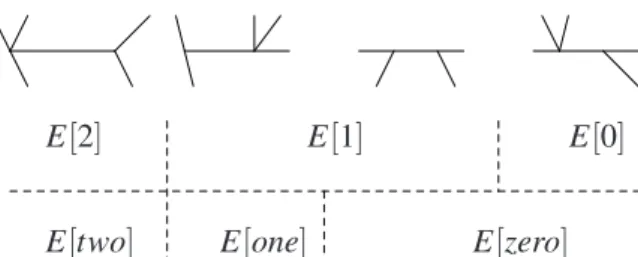
Another classification of edges: An edge can be classified by the type of its termini. One potentially useful method might be as follows: an edge is of type

[j],j_{∈ {}zero, one,two_}if exactly jof its termini are of type E0[2]. So this gives a new breakdown of E intoE[zero], E[one]and E[two], a verbal annotation which avoids confusion with the previous numeric breakdown,E[0],E[1]and E[2]. We note thatE[2]_≡

E[two], so

PE{e∈E[two]}=ε2.

We also note that E[0]_⊂E[zero] andE[one]_⊂E[1]. Also each E[1] edge can be labelled, ‘zero’ or ‘one’ from the second classification method. (see Fig.4).

This means that the edges are now classified into four types – the original E[2] and E[0] plus the two components of E[1], namely E[1 & zero] and E[1 &one] which we abbreviate as E[10]and E[11]

respectively. We also breakε1 into two terms,ε10and

E[zero]

E[one]

E[two]

E[2] E[1] E[0]

Fig. 4. In each picture, focus attention on the horizontal edge whose termini are both in view. This edge lies in the categories shown schematically below each picture. Both methods of classification are shown.

From the method stated above for the sampling of a typical edge-terminus, we have

PE0{e0∈E0[2]}=PE{e∈E[two]}

+1₂PE{e∈E[one]}

=ε2+1₂PE{e∈E[one]}. (23)

Using Eq.22and Eq.23, we find that

ε11=PE{e∈E[one]}=2 1− 2φ

θ −ε2

, (24)

ε10=ε1−ε11= 4φ

θ −ε1−2ε0. (25)

For the general planar tessellation we see that, although we now have a finer classification of edges, no extra parameter is needed;ε10andε11are not really new as they can be calculated from the parameters of our first classification. The finer classification does, however, play a role in some situations (as seen later in this section).

Linking ε2 and φ: Eqs. 24 and 25 provide inequalities which link ε2 and φ. Writing Eq. 24 as

ε2=1−2φ/θ−1₂ε11, we can create an upper bound for ε2 in terms of the ratio φ/θ. Similarly, Eq. 25 establishes a lower bound. These bounds are presented below in Eq.26and illustrated in Fig.5b.

1₋4φ

θ +ε0≤ε2≤1−

2φ

θ . (26)

Note that (ε2 = 1) =⇒ (φ = 0) from the upper inequality and (φ = 0) =_⇒ (ε2 =1) and (ε0 =0) from the lower inequality and the fact that each epsilon ∈[0,1]; so(φ=0)and(ε2=1) are equivalent, as is intuitively obvious.

The earlier examples revisited: In the STIT example,ε11= 4₃(3−4 log 2)≈0.3032 whilst ε10 = 2

3(2 log 2−1) which happens to equal ε0. Note also that ¯ℓE[10] =ℓ¯E[0], proved by the methods in Cowan

(2013), so therefore ¯ℓE[11]= (ε1ℓ¯E[1]−ε10ℓ¯E[10])/ε11= 3(3 log 2₋2)ℓ¯E/(3−4 log 2) =1.048 ¯ℓE.

ε2

θ

2φ/θ φ

1+ε0

1 2(1+ε0) 1

1 1

6

3

(a) (b)

Fig. 5.(a) The permitted range for(φ,θ)as described in the inequalities of Eq. 1. (b) The permitted range for (2φ/θ,ε2)for a given value of ε0, taken from the inequality Eq.26.

Note that ε10 = 0 and ε11 = ε1 = 10₂₁ in the Divided Delaunay tessellation D_{1, as expected from}

the description of that model (where type E[10]is an impossibility).

In the 2_×1–tiling, none of theE[1]–edges are of type E[10], soε10=0 and ε11=ε1= 4₉. Thus edges are either of type E[2] or type E[11], a feature that allows us later to compute the properties of this model combined in superposition with any isotropic model. Obviously, ¯ℓ_E[11]=ℓ¯_E[1]=1.

The example in Fig. 6: An example which demonstrates ε10 and ε11 is seen in Fig. 6; it is described and partially analysed (yieldingθ= 19₆ and

φ =5₆) in the figure’s caption. The area of the shaded region is 32 so, because of the 7 cells, 19 edges and 12 vertices associated with this area, λZ= ₃₂7, λE =

19

32 and λV = 3

8. Furthermore, of the 19 edges, 4 are type E[0], 10 areE[1]and 5 areE[2]. Thereforeε0=

4 19,ε1=

10

19 andε2= 5

19. Eq.24yieldsε11=2(1− 10 19− 5

19) = 8

19, so ε10 = 2

19 from Eq. 25. This agrees with the observed breakdown of typeE[1]into sub-types: 8 beingE[11]and 2 beingE[10].

Fig. 6.A tessellation based on congruent copies of the region shown in dark shading arranged to cover the plane. It is made stationary by ensuring that the origin is uniformly distributed within the dark region. This region measures 8_×4 and comprises 7 rectangular cells whose side lengths are of integer length, either 1, 2 or 4 units. The heavy lines within the dark region comprise 19 edges and there are 12 vertices within the region not counting those on its northern and eastern boundary (as these are counted in other copies of the region). Ten of the 12 vertices areπ-vertices (each with 3 emanating edges) and the remaining two are notπ -vertices (each having 4 emanating edges). So θ= 19₆

and φ = 5₆. The white patches, each containing two cells, are explained later in the text.

Consider firstly the top-left white patch; it contains a 4_×2 upper cell and a 2_×2 lower cell, separated by an edge of length 2 (which happens to be of type E[10]). Conditioning on the geometry of the patch, the chance that the separating edge is hit by the upper cell’s chord is 2 times the edge’s length divided by the perimeter of the upper cell, namely 1₃. For the lower cell, the conditional chance is 1₂. Given the geometry of the patch, these hitting events are independent. So the probability (given the patch geometry) that the separating edge is hit by 0,1 or 2 chords is 1₃,1₂ and 1₆ respectively. Repeating the calculation for the bottom-right patch, where the separating edge is also of type E[10], we get probabilities for 0,1 or 2 hits of ₁₀3,1₂ and

1

5 respectively, conditional on that patch’s geometry. Any hit is independently uniformly distributed along the separating edge.

As these two patches (and their equally-prevalent copies throughout the plane) contain the only type E[10]edges, we can say that the chance that a typical E[10]edge receives 0,1 or 2 hits is 1₂(1₃+₁₀3) = 19₆₀,1₂

and1₂(1₆+1₅) =11₆₀respectively. AnE[10]edgeewhich is not hit remains of typeE[10]and hit twice becomes oneE[10]plus twoE[0]edges. Hit once by the chord in the cell whose sidesequalse, it becomes twoE[10]

edges (the probability here is 19₆₀). It becomes twoE[0]

edges if the hit comes from the cell whose sides_⊃e (probability11₆₀).

The third row of Table 1 shows the resulting edge-types produced from the possible hits onE[10]edges.

The same exercise can be repeated for the eight edges that are of type E[11]. The post-division edge-types differ from those in theE[10]analysis (see Table 1), emphasising the need to break the type E[1]into its two parts. The hit probabilities can be found for the typicalE[11]edge: no hits, 103₁₈₀; two hits, ₁₈1; one hit withs=e, 19₉₀; one hit withs_⊃e, ₁₈₀29.

For the five E[2] edges, Table 1 presents the resulting edge-types and a calculation shows that there will be 0,1 or 2 hits of the typical E[2] edge with probabilities ₇₅8,11₂₅ and 34₇₅ respectively. The probabilities of 0,1 or 2 hits of the typical E[0]edge are 5₈,1₃ and₂₄1.

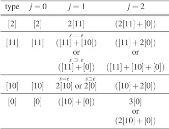
Table 1.Given the edge-type given in column one, the Table shows the types of edges that result from j hits by chords, j=0,1,2. For example, a[0]-edge hit by2 chords is subdivided into three edges; either all three will be type[0]or there will be two of type[10]and one of type[0]. Given j=2, the alternatives linked by the word ‘or’ are equally likely in all examples, but when j=1 the alternatives ‘s=e’ and ‘s _⊃e’ will have example-dependent probabilities (see text).

type j=0 j=1 j=2

[2] [2] 2[11] (2[11] + [0])

[11] [11] ([11s] + [=e10]) ([11] +2[0])

or or

s⊃e

([11] + [0]) ([11] + [10] + [0])

[10] [10] 2s[=10e]or s⊃e

2[0] ([10] +2[0])

[0] [0] ([10] + [0]) 3[0]

or

(2[10] + [0])

λ_E∗_[2]= ₇₅8λ_E[2]+λZ=113₄₈₀ ,

λ_E∗_[11]=2(11 25+

34

75)λE[2]+λE[11]=127240 ,

λ_E∗_[10]= (19₉₀+1_2×181)λE[11]+ (1960+2× 19 60+

11 60)λE[10]

+ (1₃+₂₄1)λ_E[0]=₂₈₈₀511 ,

λ_E∗_[0]= 34₇₅λE[2]+ (18029 + 1

12)λE[11]+2(1160+ 11 60)λE[10]

+ (1+2_×481)λ_E[0]= 887 2880. Adding the four intensities above yields λ∗

E = 54, a result which conforms with the simpler equation,

λ_E∗=λE+3λZ=19₃₂+3×₃₂7 =5₄.

Note that λ∗

E[1] = λE∗[11] +λE∗[10] = 407576. Also, the epsilons follow: firstly ε₂∗ = λ_E∗_[2]/λ_E∗ = 113₆₀₀, then similarly ε₁∗= 407₇₂₀ and ε₀∗ = ₃₆₀₀887. For completeness,

λ_V∗ = λV +2λZ = 1316 and λV∗[π] =λV[π]+2λZ = 34, implying thatθ∗=40₁₃ andφ∗=12₁₃.

REMARK 3: We note that the mathematics of this example is unchanged if, instead of using only horizontal and vertical chords, those which are distributed uniformly random (UR) on the set of all chords are used. The probability, given the cell’s perimeter b, that a chord hits an edge of length ℓ is

still2ℓ/b.

REMARK 4:Table 1 is universal; it holds for any tessellation and any mechanism for determining the dividing chords. So the point of our example is this: for any tessellation all four epsilons, ε2,ε0,ε11 and

ε10 are essential inputs to the calculation of post-division structure. Another input is also needed: the probabilities of 0,1 or 2 hits of the separating edge for each edge type. These probabilities were simply calculated in our example, but could be rather difficult

to find in general.

The D_{2 iterate of the Delaunay: To illustrate}

Remark 4, we consider again the Divided Delaunay tessellation. We note that the first iterate D_{1 has no}

E[10] edges, ε10 =0 being implied by the equality ofε1 and ε11. In the second iterate D2, however, we see from Table 1 that this type occurs — E[10] can arise from the division of eitherE[11],E[10]orE[0]

types. The relevant recurrences, after calculation of the hit probabilities and application of Table 1 (details omitted), are:

λ_E(2_[2)_]= 4₉λ_E(1_[2)_]+λ_Z(1)=148₂₇ρ,

λ_E(2_[11) _]= 10₉λ_E(1_[2)_]+λ_E(1_[11) _]=190₂₇ρ,

λ_E(2_[10) _]= 11₃₆λ_E(1_[11) _]+0_×λ_E(1_[10) _]+11₃₆λ_E(1_[0)_]= 121₁₀₈ρ,

λ_E(2_[0)_]= 1₉λ_E(1_[2)_]+₃₆7λ_E(1_[11) _]+0_×λ_E(1_[10) _]+37₃₆λ_E(1_[0)_]=49₃₆ρ.

From these we get the basic epsilons for D_{2: ε}(2)

2 = 148

405; ε

(2)

1 = 1620881; ε

(2)

0 = 54049. One can also show that

θ_π(2)=29₉ andµ_{V E}(2)₍₂₎=262₂₇ +256_567×37.7808_≈26.7617. We do not present results forD_{n, n>2 as analysis of}

the hit probabilities becomes very complicated.

EXAMPLES OF NESTING AND

SUPERPOSITION

These two operations which can be applied to a pair of tessellations are defined as follows.

DEFINITION 6: Consider two tessellations with framesY_1andY_{2; thesuperpositionis the tessellation}

with frame Y ₌ Y_{1 ∪}Y_{2. Object classes of} Y

are denoted by V,E,Z,S, ..., as usual, and those belonging to tessellationY_{j, j=1,2,are denoted by}

V(j),E(j),Z(j),S(j), .... A similar superscript is used for parameters of Y_{j (for example, θ}(j)_,φ(j)_{, ...), except}

when such use is redundant (as inλ(j)

E(j), whence either λ_E(j)orλ_E(j)suffices, the latter being easier to read).

In this section, Y_{1 and} Y_{2 are assumed}

independent; an exception to this is given in the next section.

DEFINITION 7: To describe nesting, we again start with a tessellation frame Y_{1. Also we have}

available the distribution of the independent frame

Y_{2, allowing us to produce independent replicates of} Y_{2 when required. Then, for each closed cell z of} Y_{1, we independently generate a tessellation} Y_2(z)

distributed as Y_{2 and add} Y_{2(z)∩z to} Y_{1. Thus}

we create a tessellation Y _{equal to} Y_{1 plus all}

‘nested components’ inside the cells of Y_{1, that is,}

Y ₌Y_{1 ∪} S

z(Y2(z)∩z) (Maier and Schmidt,2003;

Nagel and Weiss,2003). Notation is the same as that in Definition 6, with the comment that the superscripted parameters and object classes when j=2refer toY₂

and do not have a clear definition forY_{2(z)∩z when}

z_∈Z(1).

Many researchers have discussed thesuperposition and nesting of two tessellations, presenting formulae for parameters like λV and λE in the resulting process in terms of the parameters for each of the original tessellations (Santal´o, 1984; Mecke, 1984; Weiss and Z¨ahle, 1988; Maier and Schmidt, 2003; Nagel and Weiss,2003;2005). An assumption needed for reasonably pleasant formulae is that at least one of

Y_{1 or}Y_{2 should be isotropic. We too can reproduce}

(an assumption which prevails in this section). The formulae that result are as follows, using (S) and (N) to mark the superposition and nesting cases respectively.

λE=

  

 

λ_E(1)+λ_E(2)+4

πℓ¯ (1)

E ℓ¯

(2)

E λ

(1)

E λ

(2)

E (S)

λ_E(1)+λ_E(2)+6

πℓ¯ (1)

E ℓ¯

(2)

E λ

(1)

E λ

(2)

E (N) (27)

λV=



 

 

λ_V(1)+λ_V(2)+2

πℓ¯ (1)

E ℓ¯

(2)

E λ

(1)

E λ

(2)

E (S)

λ_V(1)+λ_V(2)+4

πℓ¯ (1)

E ℓ¯

(2)

E λ

(1)

E λ

(2)

E (N) (28)

We have a greater interest, however, in the effects of these operations on parameters like λ_V[π],φ and

εj. Santal´o (1984), who first analysed the effects of superposition– and others cited above who extended his analysis and introduced nesting – were not concerned with these parameters. In the theory and examples given below and in the Appendix, we focus on λ_V[π],φ and εj, j=0,1,2, while drawing on the known results Eq.27and Eq.28.

The parametersλ_V[π] andφ: Forsuperpositions it is easily seen that the onlyπ-vertices inY _{are those}

that wereπ-vertices in the initial tessellationsY_{1 and} Y_{2; no newπ-vertices are created by the intersection}

of the two frames. On the other hand,nestingproduces newπ-vertices created by the intersection ofY_{1 with}

S

z(Y2(z)∩z) whilst also retaining the original π -vertices ofY_{1and of the nested replicates of}Y_{2. These}

remarks onπ-vertices lead (with the help of Eq.31in the Appendix) to the following formulae.

λ_V[π]=   

 

λ_V(1_[π)_]+λ_V(2_[π)_] (S)

λ_V(1_[π)_]+λ_V(2_[π)_]+4

πℓ¯ (1)

E ℓ¯

(2)

E λ

(1)

E λ

(2)

E (N) (29)

The parameterφis given byλ_V[π]/λV.

Edge-types: In both contexts, we say that an edge in the resulting tessellation frame Y _{is of}Y_1-genesis

if it is a subset of the Y_{1 frame. Otherwise, it is of} Y_{2-genesis. It is important to note that an edge of}Y_i

-genesis might not be an edge ofY_{i, but only a subset}

of one.

REMARK 5:IfY_{2is side-to-side, all of the edges}

inY _ofY_{2-genesis will be of type E[2], whether}Y _is

a superposition or a nesting. IfY_{2 is not side-to-side,}

results about edge-types are usually less amenable.

A superposition example: The(2_×1)–tiling seen above plays the role of Y_{1. Its superposition partner} Y_{2is our isotropic Delaunay tessellation}D_{0, chosen to}

have parameterρ = (3π/8)2_{≈1.388 so that λ} (1) E =

λ_E(2) in conformity with Fig. 7. Therefore, in this example, Y_{2 is side-to-side and} Y_{1 has no edges of}

typesE[10]orE[0], a feature which enables an easy analysis. From this earlier analysis, we know that

λ_V(1)= 5

8, λ

(1)

E = 9

8, θ

(1)₌ 18

5 ,

λ_V(2)= 9π

2

64 , λ

(2)

E = 27π2

64 , θ

(2)_=6,

and ¯

ℓ(_E1)=4

3, λ

(1)

V[π]=

1 4, φ

(1)₌ 2

5, ¯

ℓ(_E2)=4

3, λ

(2)

V[π]=0, φ

(2)_=0.

So, from Eqs.27–29,

λV = 1

64(40+108π+9π 2₎

≈7.3, λ_V[π]=1

4,

θ =2λE

λV ≈

4.35, φ= λV[π]

λV ≈ 0.034,

λE = 9

64(8+24π+3π 2₎

≈15.9, ℓ¯E = 4 3.

Also λ_E(1_[2)_] = ₈5, λ_E(1_[11) _] = ₂1, ℓ¯(_E1_[)_2] = 8₅ and ¯ℓ(_E1_[)_11] =

1, from the earlier calculations. Thus, because every type E[11] in Y_{1, whether remaining intact or not,}

yields exactly one E[11] for Y _{(and there are no}

E[11]-type edges of Y_{2-genesis because} Y_{2 is}

side-to-side), λ_E[11] = 12. Therefore λE[2] =λE−λE[11] =

5 8+

27

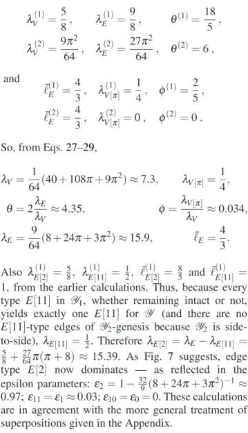
64π(π+8) ≈ 15.39. As Fig. 7 suggests, edge type E[2] now dominates — as reflected in the epsilon parameters:ε2 =1−32₉(8+24π+3π2)−1≈ 0.97;ε11=ε1≈0.03;ε10=ε0=0. These calculations are in agreement with the more general treatment of superpositions given in the Appendix.

Fig. 7.The bold line-segments form the frame of a2_×1 tiling. Superimposed on it is our Delaunay tessellation

D_{. Parameters have been chosen so the mean edge}

A nesting example: Here both Y_{1 and} Y₂

are isotropic Poisson line processes, having ‘point processes on line-transects’ with intensities ρ(1) _and ρ(2) respectively. These point processes are Poisson processes, so the tessellations have the Poisson Transect Property discussed in Remark 1. Also the typical edge in either tessellation has a length that is exponentially distributed. The relevant parameters of

Y_1andY_{2, calculated inMiles(1973) are as follows:}

λ_V(1)= π

4(ρ

(1)₎2_{, λ}(1)

E =

π

2(ρ

(1)₎2_{, θ}(1)_=4,

λ_V(2)= π

4(ρ

(2)₎2_{, λ}(2)

E =

π

2(ρ

(2)₎2_{, θ}(2)_=4,

¯

ℓ(_E1)= 1

ρ(1), λ (1)

V[π]=0, φ

(1)_=0,

¯

ℓ(_E2)= 1

ρ(2), λ (2)

V[π]=0, φ

(2)_=0.

From these, and using Eqs. 27–29 together with Lemma 3 and Eq.32, we calculate

λV =

π

4

(ρ(1)+ρ(2))2+2ρ(1)ρ(2),

λE =

π

2

(ρ(1)+ρ(2))2+ρ(1)ρ(2),

λ_V[π]=π

2ρ

(1)_ρ(2)_{, φ=} λV[π] λV

and θ= 2λE

λV

.

Using Lemma 3, Eq.32and Eq.33, we find that

λ_E[Y₁]= π

2ρ

(1) _ρ(1)_+2ρ(2)

, ℓE[Y₁]=

1

ρ(1)_+2ρ(2),

λ_E[Y₂]= π

2ρ

(2) _ρ(1)_+ρ(2)

, ℓE[Y₂]=

1

ρ(1)_+ρ(2),

and

¯

ℓE =

ρ(1)_+ρ(2)

(ρ(1)_+ρ(2)₎2_+ρ(1)_ρ(2).

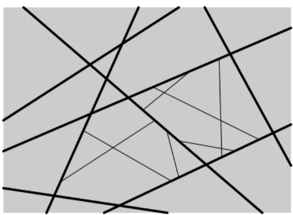
Fig.8showsY_{1and, inside two neighbouring cells}

z and z_∗ of Y_{1, the nesting by} Y_{2. We note that all}

edges of Y_{2-genesis contained in z (or in z∗) are of}

typeE[2]. The figure also shows the line-segmentz∩z∗ which was originally an edge (e say) of Y_1.

Post-nesting, it has been transformed into five edges ofY

1-genesis, but in general the types of these edges may be E[11],E[10]orE[0]depending on the positions of the hits ofe=z_∩z_∗– and whether the hits are caused by chords ofzor chords ofz_∗.

Fig. 8. The bold lines show the frame Y_{1 of a line}

process into which independent copies of a line process

Y_{2 will be nested. In order to focus attention on two}

neighbouring cells z and z_∗ of Y_{1 and the five}

post-nesting edges ofY_{1-genesis on the line-segment z∩z∗,}

we only show the nesting in these two cells of Y_1.

Inside these cells, we see the post-nesting edges ofY

2-genesis as thin lines.

BecauseY_{2 has thePoisson Transect Property,Ke}

has the Poisson distribution with mean 2ρ(2)_{ℓ, given}

the length ℓ of an edge e of Y_{1. Moreover, given ℓ}

and givenKe=k>0, these k hits are uniformly and independently positioned on the edge e and equally likely to be caused by chords inzorz_∗. Thus, thekhits create two E[11]edges, an expected (k−1)/2 edges of E[10] type and also an expected (k₋1)/2 edges of E[0] type. In Fig. 8, k=4 and we see two E[0]– edges and oneE[10]–edge, along with the twoE[11] -type edges. Whenk=0, the edge remains type E[2]. Therefore, the typical edge ofY_{1 (in this example all}

edges ofY_{1are typeE[2]) has an expected number of}

Z ∞

0 _k

∑

2 PE(1){Ke=k|ℓ} f(ℓ)dℓ

type–E[0] edges. Here, f is the probability density function ofe’s lengthℓ, known to beρ(1)_exp(−ρ(1)_ℓ)

in this example because Y_{1 is also a Poisson line}

process. Evaluating the formula above, we get

Z ∞

0 _k

∑

2

(2ρ(2)_ℓ)k_e−2ρ(2)_ℓ

k! ρ

(1)_e−ρ(1)_ℓ

dℓ

= 1

2 Z ∞

0

e−2ρ(2)ℓ₋1+2ρ(2)_ℓρ(1)_e−ρ(1)_ℓ

dℓ

= 2(ρ

(2)₎2

ρ(1)_(ρ(1)_+2ρ(2)₎.