Robust performance for arbitrary order plant under structured and unstructured uncertainties

(1)

Robust performance for arbitrary order plant under

structured and unstructured uncertainties.

1

Gursewak Singh

1

Assistant Professor (ECE) , Yadawindra College Of Engineering ,Guru Kashi Campus, Punjabi University Patiala(Punjab)

Abstract- In present paper ,I Investigated the problems of designing the PI controllers for robust performance and stability for an arbitrary-order SISO(single Input and single output) linear time-invariant plant or system concerned with the problems of both structured and unstructured uncertainities.For achieving the robust stability for plant under the effect of uncertainities, I will convert all the problems into the segments of Qusipolynomial equations. The results on H∞ PI designing or tuning are then used into a programming design techniques for obtainig the values of required PI (proportional and integral) gains (Kp,Ki). Main important charactersitic of the given method is that it constructively characterizes the entire set of tuned PI controllers. This characterization can provide the optimal tuning of PI controller for the required design.

Keywords- PI Controller , Structure uncertainity,Robust Stability, Frequency domain,Sensitivity, Unstructured uncertainity .

I INTRODUCTION

Uncertainty in any plant or system give us motivation for designing an optimal control for stabilization of plant. It provide us a platform for introducing the closed loop feedback and force us to ponder over on present research for achieving required robustness for plant. We can give a broadly classification of uncertainty in plant into two ways,Strucured and Unstructured uncertainties.A structured class of uncertainity include the Parametric perturbations. As a result, an actual deviation in physical parameter of any plant or system in control loop is parametric uncertainty or perturbations.An Unstructured class of uncertainty is considered as norm-bounded perturbations and uncertainity in system concerned with dynamics in system , truncation of models of higher frequency,linearization effects and non-linearities, etc.Systems is usually associated with both problems of unstructured and structured uncertainty.Robust stability analysis under effects of structured and unstructured uncetainties is included for external results in [1] and [2]. Plnats with parametric Uncertainties and norm-bounded perturbations, [3] showed that the robust performance analysis criteria could be determined for robust Stability under structured and unstructured perturbations. PID stabilization [5] on using given results in connection with the Generalized Kharitonov Theorem [4], [5] and [6] give us a platform for stabilizing a given interval plant family using PID ,PI and P controller.PID tuning for the ﬁxed LTI linear time-invariant system for robust stability with Unstructured uncertainties were

given in [7] and [8] ,on basis of the conclusions of complex PID stabilization recently [7]. After getting an immense motivation on earlier results or conclusions , the my main motive of this paper is to bring the conclusion on robust PID designing together [7], [8] and conclusion or analysis from parametric robust control process to give a better solution to the complex problems of designing PI controllers for robust performance and stability for systems or plants with both strucured and unstructured uncertainties. First,PI tuning for robust stability for system with mixed uncertainties are converted into all the problems into the segments of Qusipolynomial equations.The results on H∞ PI designing or tuning are then used

into a programming design techniques for obtainig the values of required PI (proportional and integral) gains (Kp,Ki).The goal of the paper is to determine the set of (Kp, Ki) that satisfies the following H∞ performance index Criteria

⃒ + ⃒ <<1 for robust sensitivity

constraint.where W1(s) and W2(s) is uncertainty weights to cover entire uncertainities, unstructured and structured uncertainty, G(s) is plant, K(s) is PI controller.

Robustness

With mixed uncertainties,LTI (SISO) linear time invariant system under variation of unwanted parameters, a robust performace become a big requirement. Main advantage of a closed-loop feedback system is its capability to reduce the sensitivity to structured and unstructured uncertainties .

III DEFINATIONS FOR CLOSED LOOP

Nominal stability (NS): system stable with no model uncertainty [9].

Nominal performance (NP): systems satisiﬁes performance requirements with no model uncertainty [9].

Robust stability (RS): system stable for “all” perturbations ∆ [9].

Robust performance (RP): system satisiﬁes performance requirements for “all” perturbations [9].

(2)

IV PRELIMINARY KNOWLEDGE OF THEOREMS

Lemma 1 consider that

P(s)= ( 1)

is stable where Q(s) , U(s) and E(s) are polynominals respectively with degree [Q(s)] = ϑ ,degree [U(s)] =μ,

degree[E(s)]=ρ , ϑ ≤ μ , ϑ ≤ ρ, c,d and j are the highest order

coefficient of Q(s), U(s), E(s) ,respectively. The Inequality . . ⃦P(jω) ⃦ <1 holds if and only if

1. . ⃦c ⃦>. ⃦j if ⃦ μ > ρ , . ⃦d ⃦>. j ⃦ ⃦ if μ < ρ or . ⃦c+d ⃦> . ⃦j ⃦ if μ = ρ

2. [ ]+ Q(s) is stable for all θ in[0,2π]

lemma 1 proof is given in [11] that is omitted here delebrately.

Let us view the about Hermite –Biehler theorem [10,11]

Consider the quasipolynomial

H(s) = (2)

where ≠0 m and n is positive integers, is real or complex number ,and , ,……… are real numbers satisfying 0< < <……… . The term is the principle term.For stability of quasiupolynomial H(s) in 2 equation ,the extended Hermite –Biehler theorem is explained as follows.

Theorem 1 [10,11].H(s) in equation (2) is stable if and only if

1. (jω) and (jω) have onl real zeros and these zeros interlace;

2. (jω) (jω) - (jω) (jω) >0 for someωϵ(-∞,+∞).

Here , (jω) , (jω) , (jω), (jω) denotes the real and imaginary parts of H(jω) and their first derivatives with respect to ω,respectively.

Theorem 2 [10,11]. Imagine that all θi„s values in (2) are

intergers and let ԓ si constant so that the coefficients of the highest degrees term in , (jω) , (jω) do not destroy at ω= ԓ. The required and sufficient conditions under which

(jω)=0 or (jω) = 0 has only roots is that ,in the interval

-2gπ+ ԓ≤ω≤2gπ+ ԓ , , (jω) or (jω) has exactly 4g + n real zeros starting with sufficiently large g ,respectively.

A quasipolynomial with general forms .

G(s) = D(s) +N(s) (3)

Where N(s) and D(s) are polynomials given by

N(s) = ( +j ) +( +j ) +……( +j )

D(s)= + +…… s +

Here , ……… , , …… , , ………..

are the real numbers and m>n.

Theorem 3 if m>n ,G(s) in equation (3) is stable if and only if

(i) has exactly 4g+m real zeros in (-2gπ-𝜀 , 2gπ-𝜀 ;

(ii) All the zeros of in (-2gπ- 𝜀 , 2gπ-𝜀) interlace with those of

Here z=𝜃𝜔 , g is a sufficient large integer , and are respectively ,the real and imaginary parts of H( ) and 𝜀 is given by

𝜀 =

(4)

In interval [-𝝅/2 ,π/2] in order to present the values if PI gains (Kp,Ki).

Figure 1 :block diagram of plant under control of PI controller [12]

In Figure 1 r is desired force ,G(s) is nominal plant , C(s) is PI controller ,y is actual force.

Where sensitivity S(s)= (5)

C(s)=K(s) = PI controller consist of kp and ki gains can be written as follows

C(s)= K(s) = kp+ (6)

(3)

G(s) = ∂(s)+jς(s) (7)

where s→jω in frequency domain.

Figure 2 :block diagram of plant under control of PI controller with structured and un-structured uncertainties [13]

In figure 2,Both structured and unstructured uncertainity are considered which are affecting the performance of plant or system G(s). For covering these uncertainties W1(s) and W2(s)

both uncertainty weights or scaling factor are considered explained below.

The SISO LTI plant with can be described as

G(s) = (8)

where N(s) and D(s) are coprime polynomials in s, defined

as

N(s)=Vm + Vm-1 +………+V1s+V0 D(s)= +Un-1 +………+ U1+U0

Here, V0, V1,Vm and U0, U1,Un-1 are real numbers, and n>m ,

where C(s)= K(s) is PI controller written in following form.

C(s) =K(s)= Kp+ here s→ jω , Write PI controller as given below.

C(j𝜔)=K(jω)= Kp+ (9)

Where W1(s) uncertainty weight or scaling foctor for

un-structured uncertainity and W2(s) uncertainty weight or scaling

foctor for structured uncertainity.∆(s) is stable transfer function which has magnitude less than 1, ∆(s)≤1.

W1(s)= and W2(s)= (10)

, , , , are real numerator and

denomiator ploynomial.

V CONDITIONS FOR ROBUST DESIGN

Step1 Imagine perturbed plant , if yes move to step 2

Step 2 Determine Kp and Ki gains to find the robust region

Step 3 Put Kp and Ki in for loop for angle of 𝛉∈ [ 0, 2𝛑]

Step 4 Select Angle for obtaining intersection of lines of magenta colour .𝛉∈ [ 0, 2𝛑] in figure 3.

Step 5 Select Condition for stability constraint given below, it must satisfy

⃒ + ⃒ <<1 (11)

Step 6 Find out robust stable and unstable region (intersections of lines) in figure-3

Step 7 Check robust stability constraint with PI controller using frequecy domain analysis.

Step 8 See figure 3,4,5

VI DESIGN METHODOLOGY

Now we will calculate the kp and ki gains with procedure given below. After calculating kp,ki gains , I will plot two regions: Robust region and Unstable region.

From equation (11), It can be re-written as follows,

⃒ <<1 (12)

Following is polynomial closed loop charactersitics equation

δ ( θ,s,kp,ki)=0 (13)

Equation (12) can be re-written as follows

= ⃒ (14)

<<1

(15)

Where θ= - in equation 15

Put equation (15) into (13)

δ ( θ,s,kp,ki)= -

(16)

Closed loop characterstic equation can be found putting equation (9) and (10) in equation (16) as in following mannner.

δ(θ,s,kp,ki)={s+(s*kp+ki)G(s)}-{(s }=0

(4)

From equation (13) ,δ( θ,s,kp,ki)=0 must satisfy the robust stability constraint in equation (11) for all boundary of θϵ [0,2π] in kp and ki region.

Put =(c+jd) is uncertainity weight for unstrucured uncertainity and =(e+jf) is uncertainity weight for strucured uncertainity and G(s) plant =∂+jσ , ∂,c,e is real part of plant and uncertainty weight and σ,d,f is imaginary part of plant and uncertainity weight , = cosθ+jsinθ and kp,ki is proportional and integral controller ,s→jω in equation (17) and break equation (17) into real and imaginary part.

kp(r)+ki(s) = -1-e*cosθ+f*sinθ (18) kp(u)+ki(v)= -e*cosθ+f*sinθ (19)

where

h=-1-e*cosθ+f*sinθ i=-e*cosθ+f*sinθ

r= ∂+[c*∂-d*ς]*cosθ-[c*ς+d*∂]*sinθ u=ς+[c*ς+d*∂]*cosθ+[c*∂-d*ς]*sinθ s=

v= (20)

Find kp and ki ,apply matrix theory in above equation (18) and (19) to find kp and ki.

kp= ,ki=

I have found kp,ki gains to find robust stability region

VII RESULTS AND CALCULATIONS

Consider plant G(s)= = (21)

And uncertainity weight selected to cover un-structured and strucured uncertainty.

W1(s)= = and W2(s)= = (22)

Robust criteria given below from equation (11)

⃒ + ⃒ <<1 (23)

Now we will select K(s) PI controller to obtain robust criteria. Kp and Ki Selected on robust region in following figure ,

For robust stability PI controller see figure 3

C(s) =K(s)= Kp+ here s→ jω

for robust stability

and K(s) = C(s) = -8076+ (24) Putting (21) ,(22), (24) equations into (23) equation,obtain magnitude of robust criteria given belo in equation (25) See figure 5

⃒ + ⃒ = -0.8685 (25)

For unstability PI controller see figure 3

C(s) =K(s)= Kp+ here s→ jω

for unstability

and K(s) = C(s) = -8076+ (26)

Putting (21) ,(22), (26) equations into (23) equation,obtain magnitude of robust criteria given below in equation (27)

See figure 4

⃒ + ⃒ = 1.341 (27)

-2 -1 0 1 2 3 4 5 6 7

x 104

-500 0 500 1000 1500 2000 2500

K

p Ki

select Kp and Ki in (Kp,Ki) region using PI controller

Unstable region Kp= 3537

Ki= 460.5

Kp= -8076 Ki= 2206

Robust region

Figure 3: Robust and unstable region design in (Kp,Ki) region

(5)

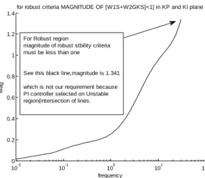
10-2 10-1 100 101 102

0 0.2 0.4 0.6 0.8 1 1.2 1.4 frequency M a g

for robust criteria MAGNITUDE OF [W1S+W2GKS]<1] in KP and KI plane

For Robust region

magnitude of robust stbility criteria must be less than one

See this black line,magnitude is 1.341

which is not our requirement because PI controller selected on Unstable region(intersection of lines.

Figure 4: Robust stability with K1 PI controller in Kp,Ki region

From figure 4, It can be observed that robust stability criteria can not be achieved,Becaude K1 PI controller selected on unstable region. see black colour line in figure 4 which reach upto 1.341 magnitude value in y-axis

10-2 10-1 100 101 102

-1 -0.9 -0.8 -0.7 -0.6 -0.5 -0.4 -0.3 -0.2 -0.1 0 frequency M a g

for robust criteria MAGNITUDE OF [W1S+W2GKS<1] in KP and KI plane

For robust stability criteria magnitude must be less than one

see on blue line,we have achieved stablity criteria,because PI controller is selected on robust region (white portion)

and Magnitude is - 0.8658

Figure 5: Robust stablity with K2 PID controller in Kp,Ki region

From figure 5,It can be judged that robust stability criteria can be achieved here ,Because K2 PI controller selected on stable robust region.See blue colour line in figure 5 ,which reach upto -0.8685 magnitude value in y-axis

Table 1.1

Robust stability criteria with control of PI controller from figure 3

(kp,ki) Value on unstable region with K1 PI controller ⃒ + ⃒ <<1

With K1 PI controller

ROBUST CRITERIA Yes or NO

(kp,ki) values on stable robust region with K2 PI controller ⃒ + ⃒ <<1

With K2 PI controller

ROBUST CRITERIA Yes or No

(3537 , 460.5) From figure 3 NO ⃒ + ⃒ = 1.341

From figure 4

( -8076 , 2206) From figure 3 Yes ⃒ + ⃒ = -0.8658

From figure 5

VIII CONCLUSION

In this paper,I proposed a practical design method of H∞ PI

controller for general single input single output LTI(linera time invariant ) system.Note that I have shown the design problem to the H∞ PI controller that has been converted

into simultaneous stabilization of the complex quasipolynomial. I have found sensitivity stability region after plotting (Kp,Ki) region (orange type shape) shown in figure 3.After selection of K1 PI controller on unstable region and K2 PI controller on stable region ,I have achieved non- stability criteria with K1 PI controller shown in figure 4 and robust stability criteria with K2 PI controller shown in figure 5.With wide use of PID and PI controller in industrial process, It is expected that the all the result calculated in this paper will contribute to the development of practical control system design.

References

[1] M. Dahleh, A. Tesi and A. Vicino, “Robust Stability and Performance of Interval Plants,” Systems & Control Letters, Vol. 19, 253-363, 1992.

(6)

[3] H. Chapellat, M. Dahleh, and S. P. Bhattacharyya, “Robust Stability Under Structured and Unstructured Perturbations,” IEEE Trans. on Automat. Contr., Vol. AC-35, 1100-1108, Oct. 1990.

[4] S. P. Bhattacharyya, H. Chapellat and L. H. Keel, Robust Control: The Parametric Approach, Upper Saddle River, NJ: Prentice Hall, 1995.

[5] A. Datta, M. T. Ho and S. P. Bhattacharyya, Structure and Synthesis of PID Controllers, London, U.K.: Springer-Verlag, 2000.

[6] M. T. Ho, A. Datta and S. P. Bhattacharyya, “Robust and Non-fragile PID Controller Design,” International Journal of Robust and Nonlinear Control, Vol. 11, 681- 708, 2001.

[7] M. T. Ho, “Synthesis of H1 PID Controllers: A Parametric Approach,” Automatica, Vol. 39, 1069-1075, 2003.

[8] M. T. Ho and C. Y. Lin, “PID Controller Design for Robust Performance,” Proceedings of the 41st IEEE Conference on Decision and Control, 1063-1067, Dec 2002.

[9] B.S Manke, .” linear control systems with matlab

applications ,”Khana publishers,pp.202-203,2005.

[10] Bhattacharyya, S.P., Chapellat, H., and L.H. Keel, “Robust Control: The Parametric Approach”, Prentice Hall, N.J., 1995.

[11] Ho., K.W., Datta, A., and S.P. Bhattacharya, “Generalizations of the Hermite-Biehler theorem,” Linear Algebra and its Applications, Vol. 302-303, 1999, pp. 135-153.

[12] Linlin Ou,Peidong Zhou,weidong Zhang and Li Yu, “H∞ Robust Design of PID controller for Arbitrary order LTI system with time delay”,2011 50th IEEE conference on decision and control and Eueropean control conference (CDC-ECC) orlando,FL,USA<December 12-15,2011.

[13] Ming-Tzu Ho and Sheng-Tsai Huang, “Robust PID Controller Design for Plants with Structured and Unstructured Uncertainty”proceedins of 22nd IEEE conference on Decision and control ,Mauii,Hawaii USA,Dec 2003.

[14] Emami, T. and J.M. Watkins, “Robust performance characterization of PID controllers in the frequency domain,”

WSEAS Transactions Journal of Systems and Control, Vol. 4, No. 5, May 2009, pp. 232-242.

[15] Bhattacharyya, S.P. and L.H. Keel, “PID controller synthesis free of analytical methods,” Proc. of IFAC 16th

Triennial World Congress, Prague, Czech Republic, 2005.

[16] K. Zhou, J.C. Doyle, K. Glover, “Robust and Optimal Control”, Prentice-Hall,London, 1996.