AUT Journal of Mechanical Engineering
AUT J. Mech. Eng., 3(1) (2019) 123-135 DOI: 10.22060/ajme.2018.14383.5724
The Effect of Road Quality on Integrated Control of Active Suspension and Anti-lock
Braking Systems
S. Aghasizade, M. Mirzaei*, S. Rafatnia
Mechanical Engineering Faculty, Sahand University of Technology, Tabriz, Iran
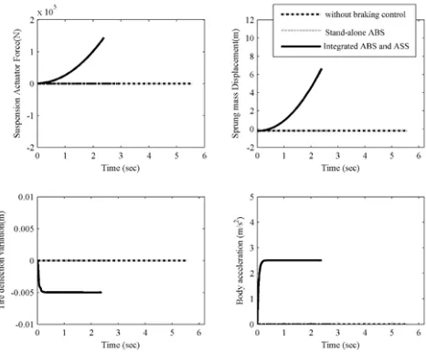
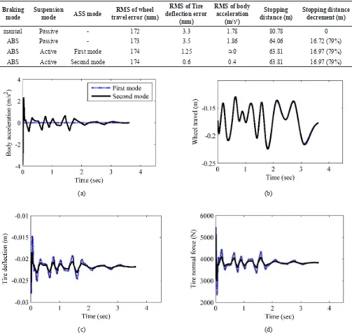
ABSTRACT: This paper investigates the effect of road quality on the control strategies of active suspension system integrated with anti-lock braking system in a quarter-car vehicle model. To this aim, two optimal control laws for active suspension system and anti-lock braking system are analytically designed using the responses prediction of a continuous 4 degree of freedom non-linear vehicle model including longitudinal and vertical dynamics. The optimal feature of the suspension controller provides the possibility of adjusting the weighting factors to meet the ride comfort and road holding criteria on roads with various qualities. It is shown that, regulating the tire deflection in a constant value to increase the tire normal load leads to instability of suspension system. Therefore, the active suspension system cannot influence on the anti-lock braking system performance on flat roads in a quarter car model. The same effect is observed for hard braking on irregular roads with good quality. In this condition, the active suspension system should be focused on the ride comfort as its first aim. However, for braking on irregular roads with poor quality, decreasing the variation of tire deflection to avoid the tire from jumping is effective in reducing the stopping distance.
Review History: Received: 30 April 2018 Revised: 23 August 2018 Accepted: 30 November 2018 Available Online: 25 December 2018
Keywords:
Integrated vehicle control Braking system Active suspension system Optimal control Road quality Tire jumping
123 1- Introduction
The purpose of integrated vehicle control is to combine and supervise two or more control systems affecting vehicle dynamic responses to enhance vehicle safety, ride comfort and handling performances. The Active Suspension System (ASS) and the Anti-lock Braking System (ABS) are two common control systems employed to attain the ride comfort and safety of vehicle during braking, respectively.
The ABS is employed to generate the maximum braking force and improves the vehicle safety by preventing the wheel from being locked. In the past, different control methods have been employed for the design of the conventional ABS controller [1-4]. In these studies, only the longitudinal dynamics is employed for braking control on flat roads. However, on rough roads, the braking can be influenced by tire normal force which is variable [5].
In normal driving conditions on rough roads, the ASS improves the ride performance by isolating the vehicle from road irregularities and reducing the sprung mass acceleration [6, 7]. For the other purpose during hard braking, the ASS controller can keep a good contact between the tire and road by controlling the tire deflection for improved safety. Because of high importance of vehicle safety, it is preferred for ASS to focus on controlling the tire deflection rather than the body acceleration when needed.
It is found that the ASS is a multi-objective system that its control strategy is dependent on driving conditions [7, 8]. For integrated suspension with other control systems, the interaction of tire normal force with tire longitudinal and lateral forces is a key factor. In what follows, some researchers
were focused on the interaction between the ASS and ABS. Lin and Ting [9] used two back-stepping controllers for decentralized integration of ASS and ABS in a quarter car model. In this study, the stopping distance was improved by increasing tire normal force, but the performance of suspension system was ignored. Wang et al. [10] investigated a Takagi-Sugeno (T-S) fuzzy neural network for integration of ASS and ABS. In another work, fuzzy and sliding mode control was used for integration of braking and steering control systems [11]. The results indicated that the proposed switching multi-layer control strategies improved the vehicle performance in different situations. In order to control the vertical and yaw motions, Vassal et al. [12] used the gain-scheduled method for both suspension and braking control systems. Kaldas and Soliman [13] investigated the influence of preview controller for both ASS and ABS systems in half car model. In this work, the ride performance of vehicle is considered in terms of ride comfort and road holding and the braking performance is evaluated in terms of braking distance. Riaz and Khan [14] designed a neuro-fuzzy based adaptive control scheme for ASS and a sliding mode control for ABS, for each station of vehicle. Zhang et al. [15] proposed a linear quarter model of active suspension system and used barrier Lyapunov function control method for both ASS and ABS systems. The results of this work showed that, the ASS can assist the ABS by increasing the tire vertical force to reduce the braking distance.
There is no doubt that a good contact between the tire and road leads to a positive interaction between suspension and braking systems [16]. This point has encouraged the researchers to enhance the ABS performance via the ASS control. However, in some cases, the possibility of this interaction has not
S. Aghasizade et al., AUT J. Mech. Eng., 3(1) (2019) 123-135, DOI: 10.22060/ajme.2018.14383.5724
124 been discussed regarding road qualities and considering all practical aspects of the problem. For example, in [9] the tire normal force is increased by controlling the tire deflection to decrease the stopping distance, is unfeasible for ASS. The feasibility of the mentioned strategy has been ignored yet. On the other hand, the integration policy may be different for braking on different roads including flat roads and irregular roads with good and poor qualities. This important issue has been paid less attention by the researchers in the past. In this paper, two strategies are proposed for optimal control of ASS and ABS based on a 4 Degree Of Freedom (DOF) non-linear quarter-car model. The minimized performance indexes related to braking and suspension control are defined separately and the control laws are analytically derived using a prediction approach. In the derived optimal control laws, the control policy of suspension system can be determined by adjusting the controller weighting factors to focus on the safety or ride comfort criteria. On the other hand, the ABS controller is designed to follow the reference wheel slip such a way that the maximum braking force can be achieved at each time. Here, the interaction of ASS and ABS during braking on flat roads and irregular roads with different qualities are investigated. Also, the feasibility of existing integrated strategies in a quarter car model is discussed considering all practical aspects of the problem. Finally, the simulation studies are conducted using the 4-DOF non-linear vehicle model excited by the standard good and poor road profiles according to ISO-8608 and the results are compared by the frequency-weighted Root Mean Square (RMS) of the vertical body acceleration according to ISO-2631 standard.
2- Modeling
2- 1- Vehicle dynamics
According to Fig. 1, a 4-DOF non-linear quarter car model including longitudinal and vertical dynamics is used to design the integrated control system.
For the vehicle model, 2-DOF are related to the vertical motion of the sprung mass, ms and un-sprung mass, mus . The other two degrees of freedom involving brake parts include the wheel angular speed, ω , and the vehicle velocity, V . In this model, fs is the nonlinear force of suspension spring and
fd is the nonlinear damper force. In addition, zr is the road profile input, zs and zu are the sprung and un-sprung mass displacements from free length of springs.
The equations of motion for sprung and un-sprung masses shown in Fig. 1 can be obtained by using Newton’s second law as,
(
)
(
)
(
)
(
)
(
)
(
)
(
)
( )
(
)
( )
( )
(
)
2 31 2 3
2 1 2 2 1 1 1 1 2
s s s u s s u s s u
d s s u s s u
st t u r
dt t u r
x t
s s s d s
u
x
s u s d st dt
x
b
t t t
i x
us
f K z z K z z K z z
f C z z C z z
f K z z
f C z z
V F
M
F R F R T
m z f
V M I VI
V R V
C
F f s
S S
f s
f m g u
m z f f f f m g u
λ λ ω λ λ λ = − + − + − = − + − = − = − = − = − − + + − = − − − + = = = + − − − − − − =
(
2 2)
(
)
2 2 2 2
if 1 1 if 1
1 tan 1
tan z r S S µF V S
Cλ Cα
ε λ α λ λ α < ≥ − + − = + (1)
(
)
(
)
(
)
(
)
(
)
(
)
(
)
( )
(
)
( )
( )
(
)
2 31 2 3
2 1 2 2 1 1 1 1 2
s s s u s s u s s u
d s s u s s u
st t u r
dt t u r
x t
s s s d s
u
x
s u s d st dt
x
b
t t t
i x
us
f K z z K z z K z z
f C z z C z z
f K z z
f C z z
V F
M
F R F R T
m z f
V M I VI
V R V
C
F f s
S S
f s
f m g u
m z f f f f m g u
λ λ ω λ λ λ = − + − + − = − + − = − = − = − = − − + + − = − − − + = = = + − − − − − − =
(
2 2)
(
)
2 2 2 2
if 1 1 if 1
1 tan 1
tan z r S S µF V S
Cλ Cα
ε λ α λ λ α < ≥ − + − = + (2) In real conditions and for hard road irregularities, fs and fd are nonlinear functions of suspension deflection, zs-zu , and suspension velocity, zs-zu , respectively, as [6]:
(
)
(
)
(
)
(
)
(
)
(
)
(
)
( )
(
)
( )
( )
(
)
2 31 2 3
2 1 2 2 1 1 1 1 2
s s s u s s u s s u
d s s u s s u
st t u r
dt t u r
x t
s s s d s
u
x
s u s d st dt
x
b
t t t
i x
us
f K z z K z z K z z
f C z z C z z
f K z z
f C z z
V F
M
F R F R T
m z f
V M I VI
V R V
C
F f s
S S
f s
f m g u
m z f f f f m g u
λ λ ω λ λ λ = − + − + − = − + − = − = − = − = − − + + − = − − − + = = = + − − − − − − =
(
2 2)
(
)
2 2 2 2
if 1 1 if 1
1 tan 1
tan z r S S µF V S
Cλ Cα
ε λ α λ λ α < ≥ − + − = + (3)
(
)
(
)
(
)
(
)
(
)
(
)
(
)
( )
(
)
( )
( )
(
)
2 31 2 3
2 1 2 2 1 1 1 1 2
s s s u s s u s s u
d s s u s s u
st t u r
dt t u r
x t
s s s d s
u
x
s u s d st dt
x
b
t t t
i x
us
f K z z K z z K z z
f C z z C z z
f K z z
f C z z
V F
M
F R F R T
m z f
V M I VI
V R V
C
F f s
S S
f s
f m g u
m z f f f f m g u
λ λ ω λ λ λ = − + − + − = − + − = − = − = − = − − + + − = − − − + = = = + − − − − − − =
(
2 2)
(
)
2 2 2 2
if 1 1 if 1
1 tan 1
tan z r S S µF V S
Cλ Cα
ε λ α λ λ α < ≥ − + − = + (4) The elastic and damping forces of tire can be modeled as,
(
)
(
)
(
)
(
)
(
)
(
)
(
)
( )
(
)
( )
( )
(
)
2 31 2 3
2 1 2 2 1 1 1 1 2
s s s u s s u s s u
d s s u s s u
st t u r
dt t u r
x t
s s s d s
u
x
s u s d st dt
x
b
t t t
i x
us
f K z z K z z K z z
f C z z C z z
f K z z
f C z z
V F
M
F R F R T
m z f
V M I VI
V R V
C
F f s
S S
f s
f m g u
m z f f f f m g u
λ λ ω λ λ λ = − + − + − = − + − = − = − = − = − − + + − = − − − + = = = + − − − − − − =
(
2 2)
(
)
2 2 2 2
if 1 1 if 1
1 tan 1
tan z r S S µF V S
Cλ Cα
ε λ α λ λ α < ≥ − + − = + (5)
(
)
(
)
(
)
(
)
(
)
(
)
(
)
( )
(
)
( )
( )
(
)
2 31 2 3
2 1 2 2 1 1 1 1 2
s s s u s s u s s u
d s s u s s u
st t u r
dt t u r
x t
s s s d s
u
x
s u s d st dt
x
b
t t t
i x
us
f K z z K z z K z z
f C z z C z z
f K z z
f C z z
V F
M
F R F R T
m z f
V M I VI
V R V
C
F f s
S S
f s
f m g u
m z f f f f m g u
λ λ ω λ λ λ = − + − + − = − + − = − = − = − = − − + + − = − − − + = = = + − − − − − − =
(
2 2)
(
)
2 2 2 2
if 1 1 if 1
1 tan 1
tan z r S S µF V S
Cλ Cα
ε λ α λ λ α < ≥ − + − = + (6) where Ks1 , Ks2 and Ks3 are the suspension spring coefficients, Cs1 , Cs2 and Cs3 are the suspension damper coefficients, Kt is the tire spring coefficient, Ct is the tire damper coefficient and u is the active suspension force determined by the control law. Note that the summation of fst and fdt cannot be positive and its positive value is saturated to zero when tire jumps. The governing equations for the motions of wheel are as follow [1]:
(
)
(
)
(
)
(
)
(
)
(
)
(
)
( )
(
)
( )
( )
(
)
2 31 2 3
2 1 2 2 1 1 1 1 2
s s s u s s u s s u
d s s u s s u
st t u r
dt t u r
x t
s s s d s
u
x
s u s d st dt
x
b
t t t
i x
us
f K z z K z z K z z
f C z z C z z
f K z z
f C z z
V F
M
F R F R T
m z f
V M I VI
V R V
C
F f s
S S
f s
f m g u
m z f f f f m g u
λ λ ω λ λ λ = − + − + − = − + − = − = − = − = − − + + − = − − − + = = = + − − − − − − =
(
2 2)
(
)
2 2 2 2
if 1 1 if 1
1 tan 1
tan z r S S µF V S
Cλ Cα
ε λ α λ λ α < ≥ − + − = + (7)
(
)
(
)
(
)
(
)
(
)
(
)
(
)
( )
(
)
( )
( )
(
)
2 31 2 3
2 1 2 2 1 1 1 1 2
s s s u s s u s s u
d s s u s s u
st t u r
dt t u r
x t
s s s d s
u
x
s u s d st dt
x
b
t t t
i x
us
f K z z K z z K z z
f C z z C z z
f K z z
f C z z
V F
M
F R F R T
m z f
V M I VI
V R V
C
F f s
S S
f s
f m g u
m z f f f f m g u
λ λ ω λ λ λ = − + − + − = − + − = − = − = − = − − + + − = − − − + = = = + − − − − − − =
(
2 2)
(
)
2 2 2 2
if 1 1 if 1
1 tan 1
tan z r S S µF V S
Cλ Cα
ε λ α λ λ α < ≥ − + − = + (8)
where R is the wheel radius, It denote the total moment of inertia of the wheel, V is the longitudinal velocity of the vehicle, λ is the wheel longitudinal slip, Tb is the braking torque, Fx is the longitudinal tire force and Mt is the total mass of the quarter vehicle. Note that, the tire radius variation is assumed to be neglected.
For driving Eq. (8), the wheel longitudinal slip during braking, V>Rω , is calculated as,
(
)
(
)
(
)
(
)
(
)
(
)
(
)
( )
(
)
( )
( )
(
)
2 31 2 3
2 1 2 2 1 1 1 1 2
s s s u s s u s s u
d s s u s s u
st t u r
dt t u r
x t
s s s d s
u
x
s u s d st dt
x
b
t t t
i x
us
f K z z K z z K z z
f C z z C z z
f K z z
f C z z
V F
M
F R F R T
m z f
V M I VI
V R V
C
F f s
S S
f s
f m g u
m z f f f f m g u
λ λ ω λ λ λ = − + − + − = − + − = − = − = − = − − + + − = − − − + = = = + − − − − − − =
(
2 2)
(
)
2 2 2 2
if 1 1 if 1
1 tan 1
tan z r S S µF V S
Cλ Cα
ε λ α λ λ α < ≥ − + − = + (9)
in which ω is the angular velocity of the wheel.
In order to describe the saturation property of the tire force in the prescribed vehicle model and because of its simplicity and its good fitness to experimental data [17], the nonlinear Dugoff’s tire model is used in this study. In the Dugoff’s
Fig. 1. 4DOF non-linear vehicle model
S. Aghasizade et al., AUT J. Mech. Eng., 3(1) (2019) 123-135, DOI: 10.22060/ajme.2018.14383.5724
125 model, the relation for longitudinal force of tire in terms of longitudinal slip, road friction coefficient and normal force of tire is as follows [1]:
(
)
(
)
(
)
(
)
(
)
(
)
(
)
( )
(
)
( )
( )
(
)
2 31 2 3
2 1 2 2 1 1 1 1 2
s s s u s s u s s u
d s s u s s u
st t u r
dt t u r
x t
s s s d s
u
x
s u s d st dt
x
b
t t t
i x
us
f K z z K z z K z z
f C z z C z z
f K z z
f C z z
V F
M
F R F R T
m z f
V M I VI
V R V
C
F f s
S S
f s
f m g u
m z f f f f m g u
λ λ ω λ λ λ = − + − + − = − + − = − = − = − = − − + + − = − − − + = = = + − − − − − − =
(
2 2)
(
)
2 2 2 2
if 1 1 if 1
1 tan 1
tan z r S S µF V S
Cλ Cα
ε λ α λ λ α < ≥ − + − = + (10) where
(
)
(
)
(
)
(
)
(
)
(
)
(
)
( )
(
)
( )
( )
(
)
2 31 2 3
2 1 2 2 1 1 1 1 2
s s s u s s u s s u
d s s u s s u
st t u r
dt t u r
x t
s s s d s
u
x
s u s d st dt
x
b
t t t
i x
us
f K z z K z z K z z
f C z z C z z
f K z z
f C z z
V F
M
F R F R T
m z f
V M I VI
V R V
C
F f s
S S
f s
f m g u
m z f f f f m g u
λ λ ω λ λ λ = − + − + − = − + − = − = − = − = − − + + − = − − − + = = = + − − − − − − =
(
2 2)
(
)
2 2 2 2
if 1 1 if 1
1 tan 1
tan z r S S µF V S
Cλ Cα
ε λ α λ λ α < ≥ − + − = + (11) and
(
)
(
)
(
)
(
)
(
)
(
)
(
)
( )
(
)
( )
( )
(
)
2 31 2 3
2 1 2 2 1 1 1 1 2
s s s u s s u s s u
d s s u s s u
st t u r
dt t u r
x t
s s s d s
u
x
s u s d st dt
x
b
t t t
i x
us
f K z z K z z K z z
f C z z C z z
f K z z
f C z z
V F
M
F R F R T
m z f
V M I VI
V R V
C
F f s
S S
f s
f m g u
m z f f f f m g u
λ λ ω λ λ λ = − + − + − = − + − = − = − = − = − − + + − = − − − + = = = + − − − − − − =
(
2 2)
(
)
2 2 2 2
if 1 1 if 1
1 tan 1
tan z r S S µF V S
Cλ Cα
ε λ α λ λ α < ≥ − + − = + (12)
In the above tire model, μ is the friction coefficient of the road, Cλ and Cα are the tire longitudinal stiffness and cornering stiffness of the tire, respectively. εr is the factor of road adhesion reduction. The Dugoff’s tire model considers the interaction of longitudinal and lateral forces of tire during combined braking and steering. For the straight-line braking, the slip angle α is applied to be zero.
It should be noted that the tire normal force Fz is the interaction point of the braking dynamics and suspension. The longitudinal braking force is directly dependent on the tire normal force. Also, Fz is the sum of fst and fdt forces in Eq. (2). This shows that the ASS can influence on the tire longitudinal dynamics by controlling the tire normal force.
2- 2- Road spectrum
Following the aim of this paper, the vehicle should be excited by different kinds of road profiles for simulating the performance of integrated braking and suspension control systems. However, in some studies [9], the road irregularity is ignored for integrated control systems and the road profile is assumed to be flat. The feasibility of integrated active suspension and braking systems on flat roads in a quarter-car model needs to be investigated.
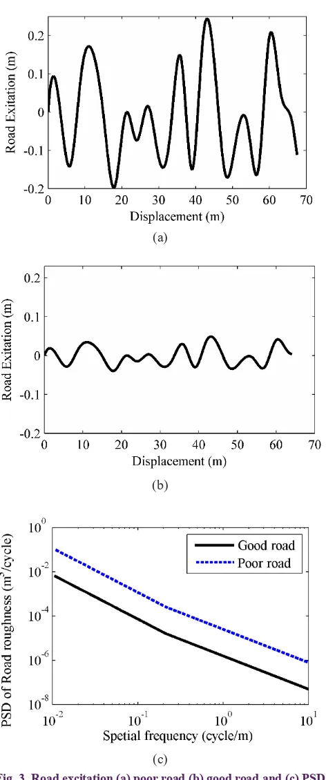
According to the standard ISO8608, the road irregularities have been classified in classes A-H based on the Power Spectral Density (PSD) [18]. The relationship between the PSD, S(Ω) , and the spatial frequency, Ω , for different classes
of road roughness is shown in Fig. 2 by two straight lines with different slopes on a logarithmic scale.
In this paper, two different profiles with the qualities of poor (D) and good (B) are chosen to evaluate the proposed control strategies. According to the PSDs of these road profiles, two random road inputs are generated and transformed in terms of displacement as shown in Fig. 3a and 3b. These inputs are generated by inverse transform of PSD functions and their heterodyning via random initial phases [18, 19]. Fig. 3c shows the PSD transform of generated random road profiles to verify the PSD inverse and heterodyning functions. Note that the transformation of the road profile expressed in terms of displacement to that in terms of time is through the vehicle speed.
3- Controller Design
For integrated ASS and ABS, two optimal control laws with adjustable weighting factors are analytically designed using the prediction of non-linear responses of a 4-DOF quarter-car model including vertical and longitudinal vehicle dynamics. Firstly, the responses of nonlinear system in the next time interval are predicted based on Taylor series expansion. Then, the control input is calculated using a continuous optimization problem defined in terms of predicted tracking or regulation errors [1, 2, 6, 7, 20]. The proposed method leads to an analytical solution for the control problem that is suitable for online implementation and reduces the requirement of real-time embedded computer hardware. In what follows, the optimal nonlinear control method is employed for the design of ASS and ABS, respectively. After that the possible interaction of these systems on different road profiles including flat road and irregular roads with the qualities described in section 2 will be investigated and discussed.
3- 1- ASS controller design
The purpose of the ASS control system is to keep the sprung mass acceleration, suspension deflection and tire deflection close to their rest situations (static equilibriums) by using a minimum external control force [5-7, 9, 18, 20]. To achieve this aim, a prediction-based method is applied for calculating the external control force.
Considering vertical dynamics, the equations of motions (Eqs. (1) and (2)) in the state space forms are derived as,
(
)
( )
(
)
( )
(
)
(
)
( )
(
)
( )
(
)
1 2 4
2 1
3 4
4 2
3
2 2
1 1 4
1
0
1 1 1 1 2 4
2 1
1 2
2 1 2 1 1
2 1
3 1 3 1 4 2
1 1 1 2 2 1 1 2! 2! s r us i i i
i i i
s us
s
r r
us
z z z
u z f
m
z z z
u z f
m
J e t h u t
e z z
z t h z t h z z
h f f u m m
u
z t h z t h f
m
h u
z t h z t h z z f z
m J η η = = − = + = − = − = + + = − + = + − + − + + + = + + + = + − + − − ∂
∑
( )
( )
(
)
(
)
( )
( )
(
)
(
)
2 11 1 1 1 2 4 1 2 2 2 2 1 1
2 1
3 3 3 1 4 2
2 2 2
1 1 2 2 3 3 4
2 2
1 1 1
1 2 3
0
2!
2!
1 ,
1 1 , ,
2! 2
r r
s us s us
u
h
u t c d e t h z z f f d e t h f
h
d e t h z z f z
c
d d d
h h h
d d d
m m m m
η η η η η η η = ∂ = + − + − + + + + − + − = − + + + = + = = − (13)
(
)
( )
(
)
( )
(
)
(
)
( )
(
)
( )
(
)
1 2 4
2 1
3 4
4 2
3 2 2
1 1 4
1
0
1 1 1 1 2 4
2 1
1 2
2 1 2 1 1
2 1
3 1 3 1 4 2
1 1 1 2 2 1 1 2! 2! s r us i i i
i i i
s us
s
r r
us
z z z
u z f
m
z z z
u z f
m
J e t h u t
e z z
z t h z t h z z
h f f u
m m
u
z t h z t h f
m
h u
z t h z t h z z f z
m J η η = = − = + = − = − = + + = − + = + − + − + + + = + + + = + − + − − ∂
∑
( )
( )
(
)
(
)
( )
( )
(
)
(
)
2 11 1 1 1 2 4 1 2 2 2 2 1 1
2 1
3 3 3 1 4 2
2 2 2
1 1 2 2 3 3 4
2 2
1 1 1
1 2 3
0
2!
2!
1 ,
1 1 , ,
2! 2
r r
s us s us
u
h
u t c d e t h z z f f d e t h f
h
d e t h z z f z
c
d d d
h h h
d d d
m m m m
η η η η η η η = ∂ = + − + − + + + + − + − = − + + + = + = = − (14)
(
)
( )
(
)
( )
(
)
(
)
( )
(
)
( )
(
)
1 2 4
2 1
3 4
4 2
3 2 2
1 1 4
1
0
1 1 1 1 2 4
2 1
1 2
2 1 2 1 1
2 1
3 1 3 1 4 2
1 1 1 2 2 1 1 2! 2! s r us i i i
i i i
s us
s
r r
us
z z z
u z f
m
z z z
u z f
m
J e t h u t
e z z
z t h z t h z z
h f f u
m m
u
z t h z t h f
m
h u
z t h z t h z z f z
m J η η = = − = + = − = − = + + = − + = + − + − + + + = + + + = + − + − − ∂
∑
( )
( )
(
)
(
)
( )
( )
(
)
(
)
2 11 1 1 1 2 4 1 2 2 2 2 1 1
2 1
3 3 3 1 4 2
2 2 2
1 1 2 2 3 3 4
2 2
1 1 1
1 2 3
0
2!
2!
1 ,
1 1 , ,
2! 2
r r
s us s us
u
h
u t c d e t h z z f f d e t h f
h
d e t h z z f z
c
d d d
h h h
d d d
m m m m
η η η η η η η = ∂ = + − + − + + + + − + − = − + + + = + = = − (15)
(
)
( )
(
)
( )
(
)
(
)
( )
(
)
( )
(
)
1 2 4
2 1
3 4
4 2
3 2 2
1 1 4
1
0
1 1 1 1 2 4
2 1
1 2
2 1 2 1 1
2 1
3 1 3 1 4 2
1 1 1 2 2 1 1 2! 2! s r us i i i
i i i
s us
s
r r
us
z z z
u z f
m
z z z
u z f
m
J e t h u t
e z z
z t h z t h z z
h f f u
m m
u
z t h z t h f
m
h u
z t h z t h z z f z
m J η η = = − = + = − = − = + + = − + = + − + − + + + = + + + = + − + − − ∂
∑
( )
( )
(
)
(
)
( )
( )
(
)
(
)
2 11 1 1 1 2 4 1 2 2 2 2 1 1
2 1
3 3 3 1 4 2
2 2 2
1 1 2 2 3 3 4
2 2
1 1 1
1 2 3
0
2!
2!
1 ,
1 1 , ,
2! 2
r r
s us s us
u
h
u t c d e t h z z f f d e t h f
h
d e t h z z f z
c
d d d
h h h
d d d
m m m m
η η η η η η η = ∂ = + − + − + + + + − + − = − + + + = + = = − (16)
S. Aghasizade et al., AUT J. Mech. Eng., 3(1) (2019) 123-135, DOI: 10.22060/ajme.2018.14383.5724
126 where z1=zs-zu , z2=zs , z3=zu-zr is the tire deflection, z4=zu is the tire vertical velocity. The functions f1 and f2 are defined in terms of suspension and tire spring and damper forces. According to the requirements of suspension system, three control variables, z1 , z2 and z3 , are taken as the outputs of the system, y1=[z1 , z2 , z3] . Therefore, a point-wise performance index minimizing the next instant output tracking errors is defined as follows [1, 4-7, 20]:
(
)
( )
(
)
( )
(
)
(
)
( )
(
)
( )
(
)
1 2 4
2 1
3 4
4 2
3
2 2
1 1 4
1
0
1 1 1 1 2 4
2 1
1 2
2 1 2 1 1
2 1
3 1 3 1 4 2
1 1 1 2 2 1 1 2! 2! s r us i i i
i i i
s us
s
r r
us
z z z
u z f
m
z z z
u z f
m
J e t h u t
e z z
z t h z t h z z
h f f u
m m
u
z t h z t h f
m
h u
z t h z t h z z f z
m J η η = = − = + = − = − = + + = − + = + − + − + + + = + + + = + − + − − ∂
∑
( )
( )
(
)
(
)
( )
( )
(
)
(
)
2 11 1 1 1 2 4 1 2 2 2 2 1 1
2 1
3 3 3 1 4 2
2 2 2
1 1 2 2 3 3 4
2 2
1 1 1
1 2 3
0
2!
2!
1 ,
1 1 , ,
2! 2
r r
s us s us
u
h
u t c d e t h z z f f d e t h f
h
d e t h z z f z
c
d d d
h h h
d d d
m m m m
η η η η η η η = ∂ = + − + − + + + + − + − = − + + + = + = = − (17)
where ei is defined as the error of each output as,
(
)
( )
(
)
( )
(
)
(
)
( )
(
)
( )
(
)
1 2 4
2 1
3 4
4 2
3 2 2
1 1 4
1
0
1 1 1 1 2 4
2 1
1 2
2 1 2 1 1
2 1
3 1 3 1 4 2
1 1 1 2 2 1 1 2! 2! s r us i i i
i i i
s us
s
r r
us
z z z
u z f
m
z z z
u z f
m
J e t h u t
e z z
z t h z t h z z
h f f u
m m
u
z t h z t h f
m
h u
z t h z t h z z f z
m J η η = = − = + = − = − = + + = − + = + − + − + + + = + + + = + − + − − ∂
∑
( )
( )
(
)
(
)
( )
( )
(
)
(
)
2 11 1 1 1 2 4 1 2 2 2 2 1 1
2 1
3 3 3 1 4 2
2 2 2
1 1 2 2 3 3 4
2 2
1 1 1
1 2 3
0
2!
2!
1 ,
1 1 , ,
2! 2
r r
s us s us
u
h
u t c d e t h z z f f d e t h f
h
d e t h z z f z
c
d d d
h h h
d d d
m m m m
η η η η η η η = ∂ = + − + − + + + + − + − = − + + + = + = = − (18) and ηi(i=1,2,3,4) ≥ 0 are weighting factors and h1 is the predictive period. zi0 is the rest situations of zi (static equilibriums) and should be tracked by each output. These reference values have been derived by solving Eqs. (13) to (16) in static situation (z2=z4=u=0). In the same way, zs0 is calculated from Eq. (1).
The predicted response for each output in the next interval, t+h1 , is approximated by a kth-order Taylor series expansion at t. The expansion order is taken to be equal to the relative degree of the system [1, 7, 20]. This selection which forces the control input to be constant in the predictive interval leads to small control efforts for nonlinear systems with small relative degrees.
According to Eqs. (13) to (16), the system dynamics has the well-defined relative degree, r1=1 for z2 and r2=2 for both z1 and z3 . Therefore, the first-order Taylor series is sufficient for z2and the second-order Taylor series is sufficient for z1 and z3 as,
(
)
( )
(
)
( )
(
)
(
)
( )
(
)
( )
(
)
1 2 4
2 1
3 4
4 2
3 2 2
1 1 4
1
0
1 1 1 1 2 4
2 1
1 2
2 1 2 1 1
2 1
3 1 3 1 4 2
1 1 1 2 2 1 1 2! 2! s r us i i i
i i i
s us
s
r r
us
z z z
u z f
m
z z z
u z f
m
J e t h u t
e z z
z t h z t h z z
h f f u
m m
u
z t h z t h f
m
h u
z t h z t h z z f z
m J η η = = − = + = − = − = + + = − + = + − + − + + + = + + + = + − + − − ∂
∑
( )
( )
(
)
(
)
( )
( )
(
)
(
)
2 11 1 1 1 2 4 1 2 2 2 2 1 1
2 1
3 3 3 1 4 2
2 2 2
1 1 2 2 3 3 4
2 2
1 1 1
1 2 3
0
2!
2!
1 ,
1 1 , ,
2! 2
r r
s us s us
u
h
u t c d e t h z z f f d e t h f
h
d e t h z z f z
c
d d d
h h h
d d d
m m m m
η η η η η η η = ∂ = + − + − + + + + − + − = − + + + = + = = − (19)
(
)
( )
(
)
( )
(
)
(
)
( )
(
)
( )
(
)
1 2 4
2 1
3 4
4 2
3 2 2
1 1 4
1
0
1 1 1 1 2 4
2 1
1 2
2 1 2 1 1
2 1
3 1 3 1 4 2
1 1 1 2 2 1 1 2! 2! s r us i i i
i i i
s us
s
r r
us
z z z
u z f
m
z z z
u z f
m
J e t h u t
e z z
z t h z t h z z
h f f u
m m
u
z t h z t h f
m
h u
z t h z t h z z f z
m J η η = = − = + = − = − = + + = − + = + − + − + + + = + + + = + − + − − ∂
∑
( )
( )
(
)
(
)
( )
( )
(
)
(
)
2 11 1 1 1 2 4 1 2 2 2 2 1 1
2 1
3 3 3 1 4 2
2 2 2
1 1 2 2 3 3 4
2 2
1 1 1
1 2 3
0
2!
2!
1 ,
1 1 , ,
2! 2
r r
s us s us
u
h
u t c d e t h z z f f d e t h f
h
d e t h z z f z
c
d d d
h h h
d d d
m m m m
η η η η η η η = ∂ = + − + − + + + + − + − = − + + + = + = = − (20)
(
)
( )
(
)
( )
(
)
(
)
( )
(
)
( )
(
)
1 2 4
2 1
3 4
4 2
3 2 2
1 1 4
1
0
1 1 1 1 2 4
2 1
1 2
2 1 2 1 1
2 1
3 1 3 1 4 2
1 1 1 2 2 1 1 2! 2! s r us i i i
i i i
s us
s
r r
us
z z z
u z f
m
z z z
u z f
m
J e t h u t
e z z
z t h z t h z z
h f f u
m m
u
z t h z t h f
m
h u
z t h z t h z z f z
m J η η = = − = + = − = − = + + = − + = + − + − + + + = + + + = + − + − − ∂
∑
( )
( )
(
)
(
)
( )
( )
(
)
(
)
2 11 1 1 1 2 4 1 2 2 2 2 1 1
2 1
3 3 3 1 4 2
2 2 2
1 1 2 2 3 3 4
2 2
1 1 1
1 2 3
0
2!
2!
1 ,
1 1 , ,
2! 2
r r
s us s us
u
h
u t c d e t h z z f f d e t h f
h
d e t h z z f z
c
d d d
h h h
d d d
m m m m
η η η η η η η = ∂ = + − + − + + + + − + − = − + + + = + = = − (21)
By using Eqs. (19) to (21), the performance index Eq. (17) can be obtained as a function of control input u . Now, the ASS control input, u , is derived by applying the optimality condition as follows:
(
)
( )
(
)
( )
(
)
(
)
( )
(
)
( )
(
)
1 2 4
2 1
3 4
4 2
3
2 2
1 1 4
1
0
1 1 1 1 2 4
2 1
1 2
2 1 2 1 1
2 1
3 1 3 1 4 2
1 1 1 2 2 1 1 2! 2! s r us i i i
i i i
s us
s
r r
us
z z z
u z f
m
z z z
u z f
m
J e t h u t
e z z
z t h z t h z z
h f f u
m m
u
z t h z t h f
m
h u
z t h z t h z z f z
m J η η = = − = + = − = − = + + = − + = + − + − + + + = + + + = + − + − − ∂
∑
( )
( )
(
)
(
)
( )
( )
(
)
(
)
2 11 1 1 1 2 4 1 2 2 2 2 1 1
2 1
3 3 3 1 4 2
2 2 2
1 1 2 2 3 3 4
2 2
1 1 1
1 2 3
0
2!
2!
1 ,
1 1 , ,
2! 2
r r
s us s us
u
h
u t c d e t h z z f f d e t h f
h
d e t h z z f z
c
d d d
h h h
d d d
m m m m
η η η η η η η = ∂ = + − + − + + + + − + − = − + + + = + = = − (22)
which leads to:
( ) ( )
( ) ( ) ( )
( ) ( )
( ) ( ) ( )
1 2 4
2 1
3 4
4 2
3 2 2
1 1 4
1
0
1 1 1 1 2 4
2 1
1 2
2 1 2 1 1
2 1
3 1 3 1 4 2
1 1 1 2 2 1 1 2! 2! s r us i i i
i i i
s us
s
r r
us
z z z
u
z f
m
z z z
u
z f
m
J e t h u t
e z z
z t h z t h z z
h f f u m m
u
z t h z t h f
m
h u
z t h z t h z z f z
m J η η = = − = + = − = − = + + = − + = + − + − + + + = + + + = + − + − − ∂ ∑ ( ) ( ) ( ) ( ) ( ) ( ) ( ) ( ) 2 1
1 1 1 1 2 4 1 2 2 2 2 1 1
2 1
3 3 3 1 4 2
2 2 2
1 1 2 2 3 3 4
2 2
1 1 1
1 2 3
0
2!
2!
1 ,
1 1 , ,
2! 2
r r
s us s us
u
h
u t c d e t h z z f f d e t h f
h
d e t h z z f z
c
d d d
h h h
d d d
m m m m
η η η η η η η = ∂ = + − + − + + + + − + − = − + + + = + = = − (23) where
(
)
( )
(
)
( )
(
)
(
)
( )
(
)
( )
(
)
1 2 4
2 1
3 4
4 2
3 2 2
1 1 4
1
0
1 1 1 1 2 4
2 1
1 2
2 1 2 1 1
2 1
3 1 3 1 4 2
1 1 1 2 2 1 1 2! 2! s r us i i i
i i i
s us
s
r r
us
z z z
u z f
m
z z z
u z f
m
J e t h u t
e z z
z t h z t h z z
h f f u
m m
u
z t h z t h f
m
h u
z t h z t h z z f z
m J η η = = − = + = − = − = + + = − + = + − + − + + + = + + + = + − + − − ∂
∑
( )
( )
(
)
(
)
( )
( )
(
)
(
)
2 11 1 1 1 2 4 1 2 2 2 2 1 1
2 1
3 3 3 1 4 2
2 2 2
1 1 2 2 3 3 4
2 2
1 1 1
1 2 3
0
2!
2!
1 ,
1 1 , ,
2! 2
r r
s us s us
u
h
u t c d e t h z z f f d e t h f
h
d e t h z z f z
c
d d d
h h h
d d d
m m m m
η η η η η η η = ∂ = + − + − + + + + − + − = − + + + = + = = − (a) (b) (c)
Fig. 3. Road excitation (a) poor road (b) good road and (c) PSD of road roughness
![Fig. 2. ISO 8608 road quality clasification [18]](https://thumb-us.123doks.com/thumbv2/123dok_us/8955576.1864944/3.595.307.549.72.280/fig-iso-road-quality-clasification.webp)
![Table 1. Parameters for the case study vehicle [1, 20]](https://thumb-us.123doks.com/thumbv2/123dok_us/8955576.1864944/6.595.315.559.610.740/table-parameters-case-study-vehicle.webp)