https://doi.org/10.5194/gmd-12-1403-2019 © Author(s) 2019. This work is distributed under the Creative Commons Attribution 4.0 License.
Implementation of the sectional aerosol module SALSA2.0
into the PALM model system 6.0: model development
and first evaluation
Mona Kurppa1, Antti Hellsten2, Pontus Roldin1,3, Harri Kokkola4, Juha Tonttila4, Mikko Auvinen1,2, Christoph Kent5, Prashant Kumar6, Björn Maronga7,8, and Leena Järvi1,9
1Institute for Atmospheric and Earth System Research/Physics, Faculty of Science, University of Helsinki,
P.O. Box 68, 00014 Helsinki, Finland
2Finnish Meteorological Institute, 00101 Helsinki, Finland
3Division of Nuclear Physics, Lund University, 22100 Lund, Sweden 4Finnish Meteorological Institute, 70211 Kuopio, Finland
5Department of Meteorology, University of Reading, Reading RG6 6BB, UK
6Global Centre for Clean Air Research (GCARE), Department of Civil & Environmental Engineering,
University of Surrey, Guildford GU2 7XH, UK
7Leibniz University Hanover, Institute of Meteorology and Climatology, 30419 Hanover, Germany 8Geophysical Institute, University of Bergen, 5020 Bergen, Norway
9Helsinki Institute of Sustainability Science, University of Helsinki, 00014 Helsinki, Finland
Correspondence:Mona Kurppa ([email protected])
Received: 18 November 2018 – Discussion started: 28 November 2018
Revised: 22 February 2019 – Accepted: 12 March 2019 – Published: 11 April 2019
Abstract. Urban pedestrian-level air quality is a result of an interplay between turbulent dispersion conditions, back-ground concentrations, and heterogeneous local emissions of air pollutants and their transformation processes. Still, the complexity of these interactions cannot be resolved by the commonly used air quality models. By embedding the sec-tional aerosol module SALSA2.0 into the large-eddy simu-lation model PALM, a novel, high-resolution, urban aerosol modelling framework has been developed. The first model evaluation study on the vertical variation of aerosol num-ber concentration and size distribution in a simple street canyon without vegetation in Cambridge, UK, shows good agreement with measurements, with simulated values mainly within a factor of 2 of observations. Dispersion conditions and local emissions govern the pedestrian-level aerosol num-ber concentrations. Out of different aerosol processes, dry deposition is shown to decrease the total number concen-tration by over 20 %, while condensation and dissolutional increase the total mass by over 10 %. Following the model development, the application of PALM can be extended to
local- and neighbourhood-scale air pollution and aerosol studies that require a detailed solution of the ambient flow field.
1 Introduction
in determining health impacts (for review, see, e.g. Kelly and Fussell, 2012). Traditionally used local urban air qual-ity models, such as Gaussian dispersion or semi-empirical street pollution models, cannot resolve these details in con-centration fields and interactions due to an inadequate rep-resentation of urban complexity and limitations in resolving any fine-scale flow structures (Tominaga and Stathopoulos, 2016).
Detailed information on the variability of urban air pol-lutant concentrations are, however, highly valuable to urban planning to design healthy living environments (Giles-Corti et al., 2016; Kurppa et al., 2018), to air quality monitoring network design, and to conducting exposure studies. There-fore, a building-resolving tool for simulating and predicting air quality in real complex urban environments in current and future conditions is needed. To determine airflow and dis-persion, computational fluid dynamics (CFDs) models, no-tably large-eddy simulation (LES), are currently the most promising methods. Compared to LES, turbulence models based on Reynolds-averaged Navies–Stokes (RANS) equa-tions can be computationally less demanding, but their ability to resolve instantaneous turbulence structures above a com-plex urban surface is shown to be clearly weaker (e.g. Anto-niou et al., 2017; García-Sánchez et al., 2018, and references within). With either method, the computational costs have been the bottleneck in extending CFD-based air quality mod-elling from tailpipe emission studies (e.g. Huang et al., 2014; Liu et al., 2011) to neighbourhood-scale studies. Fortunately, constantly increasing computational power has already al-lowed urban LES modelling for entire neighbourhoods up to 1 day or even more in a supercomputing environment (e.g. Resler et al., 2017). Currently, there are a number of RANS and LES models coupled with some chemical mechanism (Zhong et al., 2016) and a few RANS models with an aerosol module, for instance Mercure_Saturne with MAM (Albriet et al., 2010) and ANSYS-Fluent-based models (Uhrner et al., 2007; Huang et al., 2014) such as CTAG (Wang and Zhang, 2012). There is also at least one LES model including a de-tailed aerosol module (Liu et al., 2011), which, however, is only applied in a tailpipe emission study. The CTAG model has also been run in an LES mode (Steffens et al., 2013), but to date aerosol simulations have only considered dry depo-sition (Tong et al., 2016a, b) and chemical compodepo-sition has been usually ignored.
The fate of aerosol particles in the atmosphere substan-tially depends on their size distribution. Consequently, de-tailed aerosol modelling requires size-specific emission and background information as input. Estimates for background aerosol size distributions and concentrations can be attained from larger-scale models, whereas emission data are usually treated as total aerosol mass. Hence, emission size distribu-tion has to be estimated based on the source type and vehicle fleet in the case of traffic emissions. If any important emis-sion source is neglected, aerosol processes are also calculated erroneously. At the same time, as LES outperforms
tradition-ally used urban air quality models in resolving the turbu-lent wind field and pollutant dispersion, LES-based air qual-ity models produce unique information on pollutant trans-formation and dispersion processes with accurate emission estimates.
Numerical approaches to describe the aerosol size distri-bution and to solve the aerosol general dynamic equations can generally be divided into modal, moment, and sectional approaches. Modal aerosol modules (Ackermann et al., 1998; Liu et al., 2012; Vignati et al., 2004) represent the continuous aerosol size distribution as a superposition of several modes (usually log-normal distributions), whereas moment-based methods track the lower-order radial moments of the aerosol size distribution (McGraw, 1997). Both approaches are com-putationally efficient due to the small number of prognos-tic variables. However, the modal approach lacks accuracy in simulating the evolution of the aerosol size distribution, espe-cially if the standard deviations of log-normal modes are not allowed to vary (Whitby and McMurry, 1997; Zhang et al., 1999). Applying the moment approach instead requires re-solving a closure problem of the moment evolution equations (Wright et al., 2001). Furthermore, as aerosol properties are tied into moments, which are typically not observed proper-ties except for the first moments, retrieving information on aerosol properties during the simulation increases the com-putational load. In the sectional approach (Gong et al., 2003; Zaveri et al., 2008; Zhang et al., 2004), the aerosol size dis-tribution is represented as a discrete set of size bins. The sec-tional approach is flexible and accurate, but it is usually more computationally demanding due to the high number of prog-nostic variables.
To meet the needs of a high-resolution urban air quality model that can account for the complex interactions control-ling the local air quality at the neighbourhood to city scale, this article presents the implementation of the aerosol module SALSA2.0 (Sectional Aerosol Module for Large Scale Ap-plications; Kokkola et al., 2008, 2018) as a part of the PALM model system (see Maronga et al., 2015, for a description of PALM 4.0; a description of version 6.0 is envisaged in this special issue ofGeoscientific Model Development). The aim is to include aerosol dynamic processes into PALM, evaluate the model performance under different wind conditions, and study the relative impact of aerosol processes on the aerosol size distribution and chemical composition in real urban en-vironment.
2 Model description 2.1 PALM
The PALM model system (version 6.0) features an LES core for atmospheric and oceanic boundary layer flows, which solves the non-hydrostatic, filtered, incompressible Navier– Stokes equations of wind (u,v, andw) and scalar variables (sub-grid-scale turbulent kinetic energye, potential tempera-tureθ, and specific humidityq) in Boussinesq-approximated form. Note that PALM, originally developed as a pure LES code, now also offers a RANS-type turbulence parameteri-zation. PALM is especially suitable for complex urban areas owing to features such as a Cartesian topography scheme, a plant canopy module, and recent model enhancements like the so-called PALM-4U (short for PALM for urban applica-tions) components, including an urban surface scheme (first version described in Resler et al., 2017) and a land surface scheme (first description in Maronga and Bosveld, 2017). Furthermore, other PALM-4U components, such as chem-istry and indoor climate modules, have been or are cur-rently being implemented into the PALM model system to develop a modern and highly efficient urban climate model (Maronga et al., 2019). Due to its excellent scalability on massively parallel computer architectures (up to 50 000 pro-cessor cores; Maronga et al., 2015), PALM is applicable for carrying out computationally expensive simulations over large, neighbourhood-scale, and city-scale domains with a sufficiently high grid resolution for urban LES (Auvinen et al., 2017; Xie and Castro, 2006). The performance of PALM over urban-like surfaces has been successfully eval-uated against wind tunnel simulations, previous LES stud-ies, and field measurements (Kanda et al., 2013; Letzel et al., 2008; Park et al., 2015; Razak et al., 2013). Some funda-mental technical specifications of PALM are represented in Table 1.
2.2 SALSA
SALSA2.0 (referred to hereafter simply as SALSA) was selected as the basis for representing aerosol dynamics in PALM since one major criterion in its development has been limiting computational expenses without the cost of accu-racy. A major share of the expenses stem from having a large number of prognostic variables to describe the aerosol popu-lation. SALSA has been optimized for resolving aerosol mi-crophysics in a very large number of grid points, such as in global-scale climate models. Nonetheless, the same aerosol processes and model design choices are relevant at local scale.
In SALSA, the aerosol number size distribution is dis-cretized into XB size bins i based on the mean dry
par-ticle diameter Di of each bin. The number ni (m−3) and mass concentrationmc, i (kg m−3) of each chemical compo-nentcare the model prognostic variables. SALSA was
orig-inally optimized for computationally expensive large-scale climate models, and therefore the number of size bins is kept to a minimum (defaultXB=10) and only the
follow-ing chemical components can currently be included: sulfuric acid (H2SO4), organic carbon (OC), black carbon (BC),
ni-tric acid (HNO3), ammonium (NH3), sea salt, dust, and water
(H2O). Furthermore, the gaseous concentrations of H2SO4,
HNO3, NH3, and semi- and non-volatile organics (SVOCs
and NVOCs) that can condense or dissolve on aerosol parti-cles are also default prognostic variables. Nitrates and ammo-nium were not included in the original SALSA but have later been added (Kudzotsa et al., 2019). The sectional size distri-bution can be further divided into subranges 1 (Di.50 nm) and 2 (Di&50 nm). Subrange 1 consists of the smallest par-ticles assumed to be internally mixed, strongly hygroscopic, and containing only H2SO4, OC, HNO3, and/or NH3.
Sub-range 2 can contain all chemical components and it can be further divided into strongly hygroscopic (2a) and weakly hygroscopic (2b) subranges to allow for the description of externally mixed aerosol particle populations (Kokkola et al., 2018). The evolution of aerosol size distribution is repre-sented using the sectional hybrid-bin method (Young, 1974; Chen and Lamb, 1994). As a difference to the original SALSA,Diis calculated as the geometric mean diameter in-stead of the arithmetic mean. Assuming spherical particles, the latter tends to overestimate the total volumeVi=π6D
3 i, especially for larger aerosol particles whenXB∼10.
The original SALSA contains detailed descriptions for the aerosol dynamic processes of nucleation, condensation, dis-solutional growth, and coagulation, and here it has been fur-ther extended by including dry deposition on solid surfaces and resolved-scale vegetation and gravitational settling. The process of particle resuspension from surfaces is currently neglected. However, the resuspension of road dust, for ex-ample, can be included in the model as an additional surface emission (see Sect. 2.2.5).
A detailed description of the aerosol source–sink terms is given below (and in Kokkola et al., 2008 and Tonttila et al., 2017).
2.2.1 Coagulation
Coagulation decreases the aerosol number as two aerosol particles collide to form one larger particle. In SALSA, coag-ulation is solved using the non-iterative method by Jacobson (2005). Forni,
ni, t=
ni, t−1t 1+1t
XB P
j=i+1
βi, jnj, t−1t+121t βi, ini, t−1t
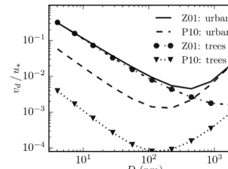
Table 1.The technical specifications of the LES model PALM.
Property Characteristics Programming language Fortran 95/2003
Discretization in space Arakawa staggered C grid (Harlow and Welch, 1965; Arakawa and Lamb, 1977)
Parallelization Two-dimensional decomposition (Raasch and Schröter, 2001); communication between processors realized using message-passing interface (MPI), with OpenMP parallelization of loops
and a hybrid mode also allowed
Sub-grid-scale closure 1.5-order scheme based on Deardorff (1980) and modified by Moeng and Wyngaard (1988) and Saiki et al. (2000)
Time-integration scheme Third-order Runge–Kutta approximation (Williamson, 1980)
Wall model By default Monin–Obukhov similarity theory (MOST, Monin and Obukhov, 1954); if the surface scheme is switched on, the momentum flux is calculated via MOST, while surface fluxes of sensible
and latent heat are calculated based on an energy balance solver for the surface temperature and a party MOST-based resistance parameterization
and, similarly, formc, i,
mc, i, t=
ρc υc, i, t−1t+1t i−1 P
j=1
βj, iυc, j, tni, t−1t !
1+1t XB P
j=i+1
βi, jnj, t−1t
. (2)
Here,t andt−1t are the current and previous time steps, βi, j is the coagulation kernel (m3s−1) of the colliding aerosol particles in size binsiandj,υc, i is the aerosol vol-ume concentration of chemical componentcin size bini, and ρcis its density. The coagulation kernelβi, j =Ecoal, i, jKi, j is the product of a collision kernel Ki, j (m3s−1) and a dimensionless coalescence efficiency Ecoal, i, j. For aerosol particles smaller than 2 µm in radius,Ecoal, i, jcan be approx-imated as unity (i.e. particles stick together) as the likelihood of bounce-off is low (Beard and Ochs, 1984). Brownian co-agulation is assumed for aerosol particles, for whichKi, j in the transition regime is calculated with the interpolation for-mula by Fuchs (1964):
Ki, j =
4π ri+rj 0p, i+0p, j ri+rj
ri+rj+ q
δ2i+δj2
+q4(0p, i+0p, j) v2p, i+v2p, j(ri+rj)
, (3)
whereri (m) is the particle radius,0p, i (m2s−1) is the par-ticle diffusion coefficient,δi (m) is the mean distance from the centre of the sphere reached by particles leaving the sur-face of the sphere and travelling a distance of particle mean free path, andvp, i (m s−1) is the thermal speed of a parti-cle in air.
2.2.2 Condensation and dissolutional growth
The condensation of gases on an aerosol particle increases the particle volume and decreases the gas-phase
concentra-tions. For water vapour, H2SO4, NVOC, and SVOC
conden-sation is calculated by applying the analytical predictor of a condensation scheme (Jacobson, 2005) in which the vapour mole concentrationCc,t at time stept after condensation is first calculated as
Cc,t=
Cc,t−1t+1t XB P
i=1
kc,i,t−1tSc,i,t0 −1tCc,s,i,t−1t
1+1t J P
i=1
kc,i,t−1t
, (4)
where kc,i,t−1t is the particle volume-dependent mass-transfer coefficient (s−1) in size bin i at the previous time stept−1t,Sc, i, t0 −1t is the equilibrium saturation ratio, and Cc, s, i, t−1tis an uncorrected saturation vapour mole concen-tration (mol m−3) of the condensing gasc. The change in par-ticle mole concentrationcc, i, tin the aerosol size biniis then given by the formula
cc, i, t =cc, s, i, t−1t+kc, i, t−1t
Cc, t−Sc, i, t0 −1tCc, s, i, t−1t, (5) which is then translated to aerosol number and mass concen-trations. The condensation and evaporation of water vapour on aerosol particles would require a very short time step to avoid non-oscillatory solutions. The applied solution used in SALSA is described in Tonttila et al. (2017).
after dissolutional growth at time steptis calculated as Cc, t=
Cc, t−1t+ XB P i=1
cc, i, t−1t
1−exp
−1t S
0
c, i, t−1tkc, i, t−1t H0
c, i, t−1t
1+
XB P i=1
H0
c, i, t−1t S0
c, i, t−1t
1−exp
−1t S
0
c, i, t−1tkc, i, t−1t H0
c, i, t−1t
.
(6) Here,Hc, i0 is the dimensionless Henry’s constant for chemi-cal compoundcin size bini:
Hc, i0 =mvcw, iR∗T Hc, (7) where mv (mol m−3) is the molecular weight of water, cw, i (mol m−3) is the mole concentration of liquid water in aerosol size bini,R∗=8.206 m3atm K−1mol−1is the uni-versal gas constant,T (K) is the ambient temperature, andHc (mol kg−1atm−1) is the Henry’s law constant estimated by
the thermodynamic model PD-FiTE (Topping et al., 2009). Finally, the new particle mole concentration cc, i, t is given by
cc, i, t=
Hc, i, t0 −1tCc, t
Sc, i, t0 −1t + cc, i, t−
Hc, i, t0 −1tCc, t Sc, i, t0 −1t
!
exp −1t S
0
c, i, t−1tkc, i, t−1t Hc, i, t0 −1t
!
, (8)
which is then translated to number and mass concentrations. The evaporation of gases from aerosol particle surfaces, with water being an exception, is not considered.
2.2.3 Dry deposition and gravitational settling
Dry deposition removes aerosol particles from air when they collide with a surface and stick to it. Here, the original scheme in SALSA allowing dry deposition on horizontal sur-faces was extended by also including deposition on vertical solid surfaces (e.g. building walls) and resolved-scale vegeta-tion. Deposition on sub-grid vegetation (e.g. grass surface) is not yet implemented. By default, dry deposition velocityvd
(m s−1) is calculated by applying the size-segregated scheme by Zhang et al. (2001) (hereafter Z01), which is the most ap-plied dry deposition scheme in numerical studies. For size bini,
vd, i=
(ρp−ρa)D 2 igGi 18ηa
| {z }
settling velocity,vc, i
+0u∗exp(−St1i/2)
Sc−i γ | {z } Brownian diffusion
+
St
i α+Sti
β
| {z }
impaction +1 2 Di A !2
| {z }
interception , (9)
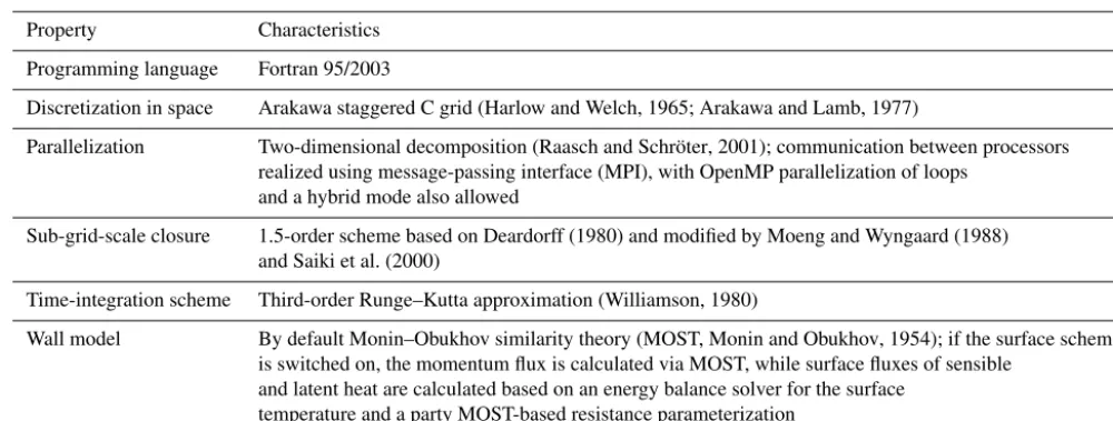
Figure 1.Normalized deposition velocity vd/u∗as a function of
aerosol particle diameter D (nm) for urban surfaces (solid and dashed lines) and deciduous broadleaf trees (dashed–dotted line with circles and dotted line with triangles) using the parameteriza-tion by Zhang et al. (Z01, 2001) and Petroff and Zhang (P10, 2010).
whereρpandρa are the particle and air densities (kg m−3),
g (m s−2) is the gravitational acceleration, Gi is the Cun-ningham slip-correction factor, ηa (kg m−1s−1) is the
dy-namic viscosity of air,0=3 andβ=2 are empirical
con-stants,u∗(m s−1) is the friction velocity of above a surface,
Sti is the Stokes number,Sci is the particle Schmidt num-ber,γ andαare empirical constants that depend on the sur-face type, andAis the characteristic radius of the different surface types and seasonal categories. Note that the aerody-namic resistance in the original Z01 formulation is not con-sidered here as LES resolves the aerodynamic effect explic-itly. For solid surfaces, u∗ is solved within PALM by
ap-plying a stability-adjusted logarithmic wind profile, whereas for the resolved-scale vegetation an estimationu∗=
√ CDU
(Prandtl, 1925), whereCDis the canopy drag coefficient and
U= √
u2+v2+w2is the three-dimensional wind speed, is
applied. Z01 has been suggested to overestimatevdfor
sub-micron particles (Petroff and Zhang, 2010; Mingxuan et al., 2018), and therefore as an alternative to Z01, the formulation by Petroff and Zhang (2010) (hereafter P10) for the depo-sition velocity can be used (see Sect. S1 in the Supplement). The different parameterizations Z01 and P10 forvdover built
surfaces and deciduous broadleaf trees during leaf-on period are visualized in Fig. 1.
Dry deposition on vegetation creates a local sink term, ∂ni
∂t = −LADvd, ini, t−1t, (10) which depends on the local leaf area density (LAD), whereas dry deposition on horizontal surfaces and building walls is implemented by means of surfaces fluxes:
The same equations apply formc, i. When not in contact with a surface, only gravitational settling contributes to dry de-position and generates a downward flux of particles, which is mainly important for large particles (D >1.0 µm) (Zhang et al., 2001; Petroff and Zhang, 2010). Dry deposition and gravitational settling are currently calculated only for aerosol particles and not for gaseous components.
2.2.4 New particle formation
In the model evaluation represented here, nucleation is as-sumed to have already occurred (Rönkkö et al., 2007; Uhrner et al., 2007), and the nucleation-mode aerosol particles are given to the model as an input. That notwithstanding, new particle formation by sulfuric acid can be taken into account by calculating the apparent rate of formation of 3 nm sized aerosol particles according to the parameterization by Ker-minen and Kulmala (2002), Lehtinen et al. (2007), or Anttila et al. (2010). To calculate the “real” nucleation rate, users can choose between the binary (Vehkamäki et al., 2002), ternary (Napari et al., 2002a, b), kinetic (Sihto et al., 2006; Riipinen et al., 2007), or activation-type (Riipinen et al., 2007) nucle-ation.
2.2.5 Emissions
Aerosol particle emissions can be given to the model as an in-put by applying three levels of detail (LOD): parameterized (LOD1, units kg m−2s−1) or detailed (LOD2, units m−2s−1) two-dimensional surface fluxes or three-dimensional sources (LOD3, units m−3s−1). Using LOD1, aerosol emissions are given as particulate mass (PM) emissions, from which the size-segregated number emissionsEni are calculated within the model implementing default aerosol size distributions and mass compositions for each emission category EC (e.g. traffic, domestic heating, etc.). LOD2 and LOD3 emission data include Eni and the mass composition per each EC, based on which the mass emission per size biniand chemical componentcare then calculated within the model. Gaseous emissions can be specified using any LOD. The time depen-dency of the aerosol emissions has not been implemented yet. 2.3 Model coupling and steering
SALSA is integrated into PALM as an optional PALM-4U module, which directly utilizes the momentum and scalar concentration fields of the parent model as input. The aerosol source–sink terms are resolved sequentially at a user-specified frequency fSALSA, while the prognostic equations
and thus the transport of aerosol number and mass as well as gas concentrations are resolved at every LES time step 1tLESin PALM. Molecular diffusion is assumed negligible
compared with turbulent diffusion and is thus ignored. Since water is a default chemical component in SALSA, PALM needs to be run in the humid mode (i.e. calculate the prognostic equation for specific humidityq). The particle
water contentmH2O, iper size binican be represented either as a prognostic variable or as a diagnostic variable and calcu-lated at each1tSALSAbased on the equilibrium solution
us-ing the Zdanovskii–Stokes–Robinson (ZSR) method (Stokes and Robinson, 1966). The feedback on temperature and hu-midity due to the condensation of water vapour on particles can be switched off. Moreover, SALSA can be run together with the available PALM-4U chemistry module to transfer the gas concentrations, while the impact of aerosol particles on radiative transfer has not been implemented yet.
2.4 Computational expenses
Eachni,mc,i, and gaseous compound introduces a new prog-nostic variable that is transported by the flow in PALM. In-creasing the number of prognostic variablesXPVfrom the
de-fault value ofXPV=6 (wind componentsu,v,wand scalars
e,θ, andq) to
XPV=6+1XPV=6+XB(XCC+1)+XG, (12)
whereXBis the number of size bins,XCCthe total number of
chemical components (aerosol phase), andXG=5 the total
number of gaseous compounds, increases the computational load tremendously. To estimate the increase in computational costs caused by significantly increasingXPV, and also
resolv-ing the aerosol dynamics, simulations over a simple test do-main of 20 m×20 m×20 m (see Fig. S1 in the Supplement) were conducted with varying set-ups for SALSA.
The relative changes in computational load per simulation are given in Table 2. AddingXB=10 size bins composed
of XCC=2 chemical components (water always present)
introduces 1XPV=35 new prognostic variables and
in-creases the original computational time by nearly a factor of 4 (run 1). Calculating the aerosol water content at each
1tSALSA instead of treating it as a prognostic variable is
even more demanding (run 2). Of all aerosol dynamic pro-cesses, coagulation is the most expensive (run 3). Including more chemical components further increases the computa-tional time (runs 8–13), which can be notably decreased by lengthening1tSALSA (runs 12–13). Considering the longer
timescales of aerosol dynamic processes compared to disper-sion (e.g. Pryor and Binkowski, 2004; Kumar et al., 2008),
1tSALSA=101t is considered to be reasonable in urban
simulations with a grid resolution of ∼1 m and 1t∼0.1. In any case, the computational expenses are multiplied when SALSA is included, which limits the size of LES model do-mains to be considered.
2.5 Initialization of the aerosol number and mass size distribution
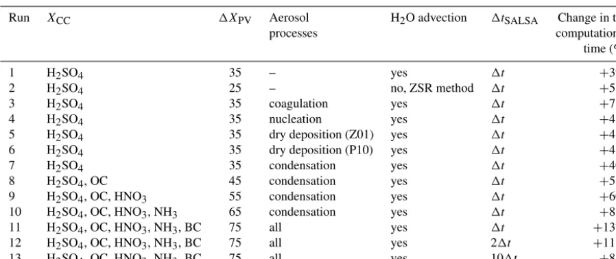
emis-Table 2.The relative change in the total computational time over a 20 m×20 m×20 m modelling domain with different configurations for SALSA. The number of simulated size binsXB=10, time step of the LES model1t≈2 s, and the total simulation time 1000 s.XCCstands
for the number of chemical components and1XPVfor the change in the number of prognostic variables.
Run XCC 1XPV Aerosol H2O advection 1tSALSA Change in the
processes computational
time (%)
1 H2SO4 35 – yes 1t +390
2 H2SO4 25 – no, ZSR method 1t +530
3 H2SO4 35 coagulation yes 1t +780
4 H2SO4 35 nucleation yes 1t +430
5 H2SO4 35 dry deposition (Z01) yes 1t +410
6 H2SO4 35 dry deposition (P10) yes 1t +410
7 H2SO4 35 condensation yes 1t +400
8 H2SO4, OC 45 condensation yes 1t +510 9 H2SO4, OC, HNO3 55 condensation yes 1t +600
10 H2SO4, OC, HNO3, NH3 65 condensation yes 1t +820 11 H2SO4, OC, HNO3, NH3, BC 75 all yes 1t +1370
12 H2SO4, OC, HNO3, NH3, BC 75 all yes 21t +1130
13 H2SO4, OC, HNO3, NH3, BC 75 all yes 101t +810
sions are defined similarly. In other words, the total number concentration is preserved in the initialization, whereas un-certainties arise when estimatingmc, i orvc, i.
Limiting XB in a sectional aerosol module is a simple
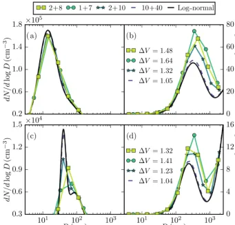
method to reduce computational costs and memory demand. However, this results in an inevitable loss of accuracy as the aerosol size range covers many orders of magnitude from a few nanometres to several micrometres. To test the sensitiv-ity of the representation of the aerosol number and mass size distribution to XB, four different configurations are tested
(Fig. 2). All configurations cover particles from 3 nm to 2.5 µm, and subrange 1 includes particles up to 10 nm. The default configuration containsXB=10 with two bins in
sub-range 1. The second configuration containsXB=8 and only
one bin in subrange 1, whereas the third configuration con-tains two additional bins in subrange 2 compared to the de-fault configuration. Additionally, an ideal configuration with XB=50 was tested.
The total aerosol particle volume concentrationV is highly sensitive to XB, and the rate of overestimation increases
with decreasing XB (Fig. 2). Overestimating particle
vol-ume causes errors in, for instance, calculating the coagula-tion kernel, gas-to-particle mass transfer, and deposicoagula-tion ve-locity. Furthermore, the ability of a sectional module to cap-ture narrow feacap-tures in a size distribution (e.g. in Fig. 2c) improves with higher XB. To compromise between
compu-tational costs and modelling accuracy, XB=10 is used in
this evaluation study.
3 Model evaluation set-up 3.1 Case description
The performance of the SALSA module in PALM is eval-uated against measurements of the vertical variation of the aerosol number size distribution and concentrations in a street canyon (Pembroke Street) in central Cambridge, United Kingdom, over consecutive 24 h on 20–21 March 2007 (Kumar et al., 2008, 2009). During the measurement campaign, the predominant wind direction (WD) was from the northwest and perpendicular to the street canyon. Fur-thermore, there is a large pedestrian area upwind of the site with no traffic emissions, and hence emissions from adjacent streets were unlikely to affect the measurements. The build-ing height is around 14–18 m on the upwind and 11–15 m on the downwind side of the street canyon (Fig. 3).
Aerosol size distributions in the size range D=5– 2738 nm were measured pseudo-simultaneously at four heights (z=1.00, 2.25, 4.62, and 7.37 m above ground level, a.g.l.) using a fast-response differential mobility spectrome-ter (DMS500). The measurement location was on the north-western side of Pembroke Street around 66 m from the clos-est intersection in the southwclos-est. Traffic volumes along the street were simultaneously measured. Moreover, 30 min av-eraged meteorological data, including wind speed (U) and direction, ambient air temperature (T), and relative humid-ity (RH), were measured 40 m a.g.l. at some 500 m from the sampling site. For more information on the measurements, refer to Kumar et al. (2008).
Figure 2. A sectional representation of the aerosol number dN/d logD (cm−3) (a, c)and volume dV /d logD(µm3cm−3)(b, d)size distribution as a function of particle diameterD(nm) in SALSA for typical polluted urban(a, b)and hazy rural conditions(c, d)(Zhang et al., 1999). Top legend: (number of size bins in subrange 1) +(number of size bins in subrange 2). The continuous log-normal size distribution is given by a solid black line.1V is the total volume concentration relative to the continuous log-normal size distribution.
of thermal and vehicle-induced turbulence (VIT) on pollu-tant transport. The evening and night-time periods represent time after sunset, while the morning measurements were con-ducted under partly cloudy conditions.
3.2 Model domain and morphological data
Simulations are conducted over a domain of a 512×512×128 grid box with the measurement site approximately at the centre of the domain (Fig. 3). A uniform grid spacing of 1x,y,z=1.0 m is applied within the lowest 96 m, and above the vertical grid1zis stretched by a factor of 1.04, resulting in a total domain height of around 164 m and a maximum 1z,max≈3.5 m.
The building-height and vegetation maps for the study area were constructed from 1 m horizontal resolution digital sur-face models (DSMs) and digital terrain models (DTMs) (En-vironment Agency UK data archive) following Kent et al. (2018). First, the DTM was subtracted from the DSM to set the terrain height to zero. Next, buildings were separated from other surface elements using a building footprint dataset
from the OS MasterMap®Topography Layer (Ordnance Sur-vey 2014). The vegetation map was formed from the remain-ing pixels by first removremain-ing the residue pixels around build-ings and then performing dilation of the raster map to remove holes and unify vegetated areas. Only vegetation elements higher thanzv,min=4.0 m were included in the simulations.
They were modelled as springtime deciduous broadleaf trees with a constant LAD=0.6 m2m−3 fromzv,min to the tree
top. This LAD value was estimated as a lower limit for urban street trees in northern Europe in spring (Gillner et al., 2015). Excluding the details of local vegetation is acceptable since there are no trees close to the measurement site and overall the amount of vegetation is low.
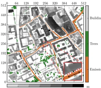
Figure 3.Visualization of the simulation domain. The building height (m) is shown in grey shades, and the location of trees and emissions are in green and copper, respectively. The evaluation domain is marked with a red square. In the zoomed figure, the black cross indicates the measurement location and the red crosses the additional points at which the model output is evaluated against measurements. The grid represents the horizontal model grid. Data sources: elevation maps – Environment Agency (UK) data archive; land use footprints – Ordnance Survey 2014.
3.3 Pollutant boundary conditions: emissions and background concentrations
In the simulations, a total aerosol number emission factor EFn=1.33×10¹⁴km−1vehicle−1is used (Table 3), which is an estimate specific to the measurement site (Kumar et al., 2009). EFnwas distributed to a representative aerosol num-ber size distribution with the shape estimated from the mea-sured size distribution at the lowest level z=1.0 m dur-ing each simulation time (see Sect. S3). Aerosol emissions are assumed to be composed of mainly black (48 %) and organic carbon (48 %) and some H2SO4 (4 % of the
to-tal mass) (Maricq, 2007; Dallmann et al., 2014). Emission factors of gaseous compounds are instead calculated using the fleet-weighted road transport emission factors for 2008 by the National Atmospheric Emissions Inventory (NAEI; Walker, 2011) and the following fleet composition: 75 % petrol and 19 % diesel passenger cars, 1 % buses, 3 % light and 1 % heavy-duty diesel vehicles, and 1 % motorcycles. Since no EFH2SO4 or EFSVOCis given by NAEI, the follow-ing estimates were applied: EFH2SO4 =0.1EFSO2 (Arnold et al., 2006, 2012; Miyakawa et al., 2007) and EFSVOC=
0.01EFNMOG (Zhao et al., 2017), where NMOG stands for
non-methane organic gases. The latter is rather conservative compared to emission rates applied by Albriet et al. (2010) for a light-duty diesel truck. Both aerosol and gaseous emis-sions are introduced as constant fluxes per unit area.
Table 3.Emission factors (EFs) applied in the simulations for all gaseous compounds and aerosol numbern.
H2SO4 HNO3 NH3 NVOC SVOC n
(g km−1vehicle−1) (km−1vehicle−1) EF 2.5×10⁻⁴ 0.0 4.2×10⁻² 0.0 2.5×10⁻³ 1.33×10¹⁴
decycling method, in which constant background concentra-tions are fixed at the lateral boundaries.
3.4 Flow boundary conditions
In all simulations, a neutral atmospheric stratification is as-sumed for simplicity as no information on the atmospheric stratification or boundary layer height was available. Thus, a constantθ=T (z=40 m) (Table 4) is applied throughout the domain. The flow is driven by an external pressure gra-dient force above z=120 m. The gradient was set so that the horizontal mean U (z=40 m) over the whole simula-tion domain equals (±0.1 m s−1) the measuredU (Table 4; see Fig. S7 for vertical profiles). Furthermore, the domain height was 164 m for all simulations. This is>13 h, where h=12.08 m is the mean building height over the domain, which should be enough to correctly resolve the small-scale turbulent structures within the urban canopy (Coceal et al., 2006).
Cyclic lateral boundary conditions are applied for the flow, q, ande, which is reasonable since the surroundings do not notably differ from the simulation domain. A Neumann (free-slip) boundary condition is applied at the top boundary and also at the bottom and top for all scalars. The roughness height is z0=0.05 m (Letzel et al., 2012) and the drag
co-efficient applied for the trees is CD=0.5 (see Kent et al.,
2017, and references within). 3.5 Simulations
Baseline simulations used to evaluate the performance of the model in the morning, evening, and at night are conducted with the default number of aerosol size bins XB=2+8
(see Sect. 2.5). All aerosol processes, except nucleation, are switched on, and the following chemical components are in-cluded: H2SO4, OC, BC, HNO3, and NH3. All aerosol
parti-cle are assumed to be internally mixed and hygroscopic, and thereby no subrange 2b was applied.
In addition to the base run, the sensitivity to different aerosol processes and the number of size binsXBwas
exam-ined for the morning simulation. Firstly, the following four simulations withXB=2+8 are conducted: no aerosol
pro-cesses (NOAP), only coagulation (COAG), only dry deposi-tion (scheme Z01) on solid surfaces and vegetadeposi-tion (DEPO), and only condensation (COND). In the first three, particles are assumed to constitute only OC in order to limit computa-tional costs, given that coagulation and dry deposition do not
depend on aerosol composition. COND is instead performed with an identical set-up to the baseline simulation, except that other processes were switched off. Secondly, the sensitivity toXBis tested by replicating the baseline morning
simula-tion with lessXB=1+7 (LB) and more binsXB=2+10
(MB).
The advection of both momentum variables and scalars was based on the fifth-order advection scheme by Wicker and Skamarock (2002) together with a third-order Runge–Kutta time-stepping scheme (Williamson, 1980). The pressure term in the prognostic equations for momentum was calculated using the iterative multigrid scheme (Hackbusch, 1985). In order to enable similar flow conditions for all simulations, feedback to PALM was switched off; i.e. changes in spe-cific humidity due to the condensation of water on aerosol particles were not allowed. Thereforeq also remained con-stant. Here, 1tSALSA=1.0 s in all simulations, which is a
safe choice since the turbulence timescale is smaller than any aerosol process timescale (Kumar et al., 2008).
Simulations were conducted with the PALM model revi-sion 3125. This was a model verrevi-sion prior to the 6.0 release, but reproducibility with version 6.0 was ensured by repeat-ing the NOAP simulation. All simulations were first run for 2 h to create a quasi-stationary state of the flow, after which SALSA was switched on and run for 70 min. Data output was collected within the last 60 min with a 0.5–1 Hz fre-quency. Simulations were performed on the Centre for Sci-entific Computing (CSC) Taito supercluster. Using 64×64 Intel Haswell processor cores, one 70 min long simulation with SALSA required between 17 h (NOAP) and 52 h (MB) of computing time.
4 Results
Table 4.Prevailing wind speedU, air temperatureT, and relative humidity RH atz=40 m a.g.l., with the applied external pressure gradient force and traffic rates for each simulation hour. Wind direction is always from the northwest (WD=315◦).
Simulation U T RH Pressure gradient in Traffic rate (m s−1) (K) (%) x,ydirections (Pa m−1) (vehicle h−1) Morning 4.30 277 64 −0.00630, 0.00630 895 Evening 3.94 274 90 −0.00515, 0.00515 380 Night 2.24 272 93 −0.00164, 0.00164 306
4.1 Baseline simulations
To give a general picture of aerosol particle concentrations and dispersion in this study, Fig. 4 illustrates the modelled total aerosol number concentrations Ntotand wind speedU
atz=3.5 m a.g.l. for all baseline simulations. The horizon-tal distribution ofNtot is shown to follow that of emissions
(see Fig. 3) and, for instance, courtyards remain relatively clean. Nevertheless, wind controls the dispersion, which is seen as up to 70 % higherNtot inside the street canyons for
the calmer night-time compared to the more windy evening simulation (see Fig. S8) despite the lower emission rates at night. Interestingly, pollutant accumulation occurs close to the measurement site within the evaluation domain.
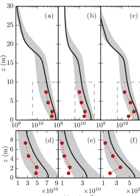
The modelled mean vertical profiles ofNtotcompare well
against the measured values (Fig. 5), especially in the morn-ing. Indeed, the additional six profiles are also generally within a factor of 2of observations (see Fig. S9). The rate of change in Ntot in the vertical is correctly modelled
ex-cept for a measured increase in concentrations within the lowest 2 m. Despite the modelled Ntot being 50 %–100 %
higher than measured in the evening (Fig. 5b), concentra-tions are of the same order of magnitude. This deviation from measurements is comparable to typical differences in measured aerosol number concentrations with different in-struments (Ankilov et al., 2002; Hornsby and Pryor, 2014). Comparing the mean values of all seven modelled profiles, their variation is shown to be larger than that between the measured and modelledNtotat the exact measurement
loca-tion.
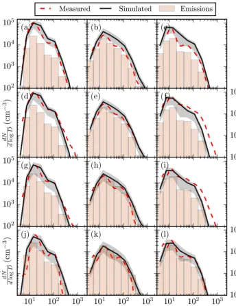
Naturally, the coarse sectional representation of the aerosol size distribution with XB=10 means some details,
such as a drop in concentrations atD≈60 nm (Fig. 6), can-not always be captured by the model. Furthermore, omitting any emission sources can produce error. For instance, an un-derestimation of the number of particles larger than 20 nm at z=2.25 m andz=4.62 m in the night-time (Fig. 6b and c) could stem from excluding some elevated sources, such as tailpipe emissions of trucks. Nonetheless, the model predic-tions are mainly within a factor of 2 of the measurements (see Fig. S10). The size distributions display very similar shapes to that of emissions, showing that the result is very sensitive to the quality of the input emission data.
Figure 4.Total aerosol number concentrationNtot (m−3,a, c, e)
and wind speed U (m s−1, b, d, f) at z=3.5 m for the
morn-ing(a, b), evening(c, d), and night-time simulation(e, f)over the
Figure 5.Measured (red circles with a dotted line) and modelled (black solid line and grey shaded area) vertical profiles of total aerosol number concentrationNtot (m−3) for the morning(a, d),
evening(b, e), and night-time(c, f)simulation.(d, e, f)Ntotin the
lowest 10 m (area marked with a black dotted line ina, b, c) using a linear scale on thexaxis. The black solid line shows the mean verti-cal profile at the measurement location and the grey shaded area the range of mean vertical profiles at six additional evaluation points within the evaluation domain.
At the same time, a mismatch with the measurements near the surface is to be expected, as the LES technique lacks re-liability close to walls. Maronga et al. (2015), for instance, showed that the turbulent flow over a homogeneous surface is not well-resolved for the lowest six grid points, which cor-responds to the lowest 5 m in these simulations. In that con-text, the modelled concentration fields agree exceptionally well with the measurements.
4.2 Sensitivity tests
4.2.1 Role of different aerosol processes
At the temporal and spatial scales applied in the simulations, dry deposition changes the total aerosol number concentra-tions most, with a relative difference1Ntot<−20 %,
espe-cially in areas with vegetation but also in the wake of
build-Table 5.Mass fractions of different chemical compounds for the
aerosol background, emissions, and simulated concentrations for the COND simulation. The values are averaged over the whole eval-uation domain withinz <30 m.
SO24− OC BC NO−3 NH+4 Background 0.09 0.24 0.64 0.0 0.03 Emission 0.04 0.48 0.48 0.0 0.0 Simulated: COND 0.05 0.36 0.49 0.08 0.01
ings (Fig. 7). Coagulation (COAG) changes Ntot only by
less than 1 %. The impact of condensation and dissolutional growth (COND) onNtotis negligible, as expected, since
con-densation only grows particles (Kumar et al., 2011). Neglecting all aerosol processes overestimates Ntot (see
Fig. S11), and therefore including dry deposition is essential for modelling realisticNtot. Above the roof level (z&15 m),
the role of dry deposition starts to weaken (Fig. 8), which is also attributable to lower aerosol concentrations. The small-est aerosol particles are most strongly affected by aerosol processes independently of modelling height (Fig. 9): this is because more efficient Brownian diffusion leads to higher deposition velocitiesvd (see Fig. 1) and coagulation rates.
Furthermore, the smallest particles grow through condensa-tion and dissolucondensa-tional growth, which instead leads to less ef-ficient removal by dry deposition. The impact of dry deposi-tion and, to a lesser extent, coaguladeposi-tion decreases with height, and above the roof level the observed1Ntotis likely due to
aerosol processes acting upwind of the measurement site. While condensation and dissolutional growth do not di-rectly affect the number concentrations, the total mass and chemical composition of aerosol particles are shown to change. Over the whole evaluation domain, condensation and dissolutional growth increase PMtot by over 10 % below the
roof height (Fig. 10). Comparing the initial chemical com-position of the background aerosol concentrations and emis-sions (Table 5) with the modelled composition shows that the mass fraction of nitrates has especially increased, from 0 % to 8 %. This increased particulate mass of nitrates originates solely from the condensation of background gaseous HNO3
as there are no traffic-related emissions of gaseous HNO3.
The simulated mass fraction of BC is very close to that of the aerosol emissions, while other mass fractions that also change due to condensation and dissolutional growth vary more. Deposition decreases PMtot, but the relative change is
clearly lower than forNtot, as the smallest particles, which
are most affected by dry deposition, represent only a tiny share of the total mass.
4.2.2 Number of size bins
Further decreasing the number of aerosol size bins XB is
Figure 6.Measured (red dashed line) and simulated (black) aerosol number size distribution dN/d logD(cm−3) as a function of particle diameterD(nm) in the morning (first column:a, d, g, j), evening (second column:b, e, h, k), and at night (third column:c, f, i, l) at levels
z=1.00, 2.25, 4.62, and 7.37 m (top to bottom). The shape of the number size distribution for the emissions is given with bars (not in units cm−3). The black solid line shows the mean value at the measurement location and the grey shaded area the range of mean values at six additional evaluation points within the evaluation domain.
XB=1+7 (LB), while settingXB=2+10 (MB) increases
the CPU time by+18 % compared to the baseline simulation in the morning. However, as shown in Sect. 2.5 and Fig. S12, the capability to describe the details of aerosol size distribu-tion drops rapidly when decreasingXB.
Despite the background Ntot and total aerosol number
emissions EFnbeing equal for the baseline, LB, and MB
sim-ulations, modelled Ntot values are not equal (Fig. 11). The
difference is entirely attributable to the dissimilar effective-ness of aerosol processes with a lower (LB) and higher (MB)
level of detail in representing the aerosol size distribution. Interestingly, using fewer size bins (LB) has a very minor impact on the horizontal field ofNtot, while more bins (MB)
result in|1Ntot|>5 %. This is still smaller than1Ntot due
to deposition.
distribu-Figure 7.Relative difference in the total aerosol number concentra-tion1Ntot(%) atz=3.5 m compared to NOAP for the(a)COAG,
(b)DEPO,(c)COND, and(d)baseline simulation in the morning.
tion is calculated from the sectional number size distribution, which is different for all simulations.
5 Discussion and conclusions
This article represents a novel, high-resolution, LES-based urban aerosol model that resolves aerosol particle concentra-tions, size distribuconcentra-tions, and chemical compositions at spatial and temporal scales of 1.0 m and 1.0 s for entire neighbour-hoods.
An evaluation study of the vertical variation of the aerosol number size distribution and total number concentration in a simple street canyon in central Cambridge, UK, shows good agreement against measurements. The model can pre-dict the dilution of concentrations in the vertical as well as the number of aerosol particles in different size bins generally within a factor of 2 of observations. The spatial distribution of aerosol concentrations is mostly determined by the flow and emissions. As regards the individual impact of aerosol dynamic processes, dry deposition is shown to decrease lo-cal number concentrations by over 20 %, which is nonethe-less at the lower end of1Ntot= [−35,−15]% estimated by
Huang et al. (2014) for an open space with traffic.
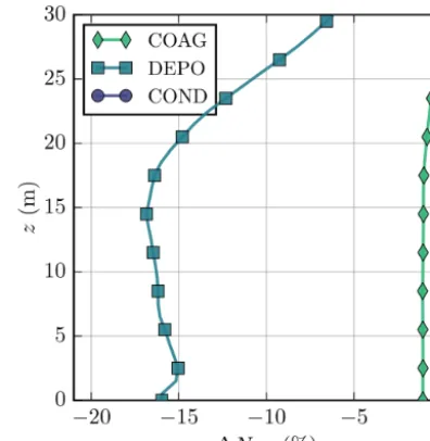
Coagu-Figure 8. Relative difference in the vertical profile of the total
aerosol number concentration1Ntot(%) compared to NOAP
sim-ulation for COAG (diamonds), DEPO (squares), and COND (cir-cles) simulations in the morning. The difference is averaged over all seven evaluation points.
lation has a very minor impact, which agrees with previous timescale analyses (Kumar et al., 2009; Zhang et al., 2004) and CFD modelling studies (Albriet et al., 2010; Huang et al., 2014; Wang and Zhang, 2012). Condensation and dissolu-tional growth increase particulate mass by over 10 %. The role of aerosol dynamic processes is shown as important for both number and mass, especially in areas with low wind speeds, such as in courtyards and the shelter of trees. Fur-thermore, comparing six additional modelling profiles to the measured one shows the limited representativeness of point measurements and supports performing air quality modelling which also gives the spatial variability of concentrations.
With increasing modelling complexity, the number of po-tential sources of modelling uncertainty is augmented. One of the largest sources of uncertainty is related to the quality of the emission data. A major reason to evaluate the aerosol model against the dataset by Kumar et al. (2008) was that the measured concentrations were mainly affected by traffic emissions along Pembroke Street, which simplified the emis-sion estimations.
Figure 9.Relative difference in the aerosol number concentration1N(%) compared to NOAP as a function of aerosol particle diameterD
(nm) at levels(a)z=3.5 m,(b)z=10.5 m,(c)z=20.5 m, and(d)z=40.5 m in the morning. The difference is averaged over all seven evaluation points.
Figure 10.Relative difference in particulate mass1PMtot(%)
com-pared to NOAP for COAG, DEPO, COND, and the baseline simu-lation within the whole evaluation domain in the morning.
Further arguments for applying the selected dataset were the availability of measurements of the vertical variability of aerosol number size distribution at high temporal resolution, but also the simplicity of the urban morphology at the mea-surement location. The influence of aerosol dynamic pro-cesses on aerosol concentration is determined by their size distribution, and thus measurements only of the total number concentration or particulate mass (e.g. Weber et al., 2006) were considered insufficient for this model evaluation. To our knowledge, there are only a few datasets on the vertical variation of the aerosol size distribution in an urban environ-ment (Kumar et al., 2008; Li et al., 2007; Marini et al., 2015; Quang et al., 2012; Sajani et al., 2018). Of these datasets, the measurement location of Kumar et al. (2008) in a street
Figure 11.Relative difference in the total number concentration
1Ntot(%) atz=3.5 m compared to the baseline simulation for the
(a)LB and(b)MB simulation in the morning.
canyon with no urban vegetation was simple enough for the first evaluation study. Modelling individual street trees and their aerodynamic impact without exact information on the distribution of leaf area introduces another source of uncer-tainty for resolving the flow. Furthermore, dry deposition is strongly tree species dependent (e.g. Popek et al., 2013; Sæbø et al., 2012) and therefore sensitive to the correct mod-elling of different species. Finally, high-resolution topogra-phy and land use information were freely available for this specific site.
At the same time, no high-resolution evaluation data for the flow were available, and therefore the modelling set-up was kept as simple as possible. Hence, the thermal and vehicle-induced turbulence was excluded from the simula-tions. The increase inNtot for z=1.0–2.25 m observed in
sources of turbulence. Kumar et al. (2008) argued that the in-crease is likely due to more efficient dry deposition near the surface or the complex dispersion pattern within the canyon caused by both topography and vehicle-induced turbulence.
Keeping in mind the aforementioned uncertainties and re-quired computational resources, the presented model pro-vides a novel and flexible tool to study, for example, how the shape, size, and location of urban obstacles affect air pollu-tant transport and transformation at a neighbourhood scale. For instance, the potential of urban vegetation to improve air quality by acting as a biological aerosol filter (Beckett et al., 1998) depends on the size-dependent deposition veloc-ity of aerosol particles, which is explicitly calculated within the model. The model can also provide information at high enough resolution to perform air pollutant exposure studies or to design a representative air pollution monitoring net-work. The aerosol module SALSA can be further coupled with an online chemistry module, which are both embedded in the PALM model system as so-called PALM-4U compo-nents. This will extend the applicability of the model from aerosol processes to more complex chemical processes and will allow researchers to examine different urban processes simultaneously such as radiation or thermal comfort. More-over, ongoing model development aims at extending the ap-plication of the model from supercomputing environments to personal PCs in future (Maronga et al., 2019).
Code and data availability. The PALM code, including the sec-tional aerosol model SALSA, can be freely downloaded from http://palm.muk.uni-hannover.de (last access: 29 March 2019). The distribution is under the GNU General Public License v3. More about the code management, versioning, and revision con-trol of PALM can be found in Maronga et al. (2015). The ex-act version of the source code used in this study is addition-ally freely available at https://doi.org/10.5281/zenodo.2575325. The stand-alone version of the SALSA model is freely avail-able at https://github.com/UCLALES-SALSA/SALSA-standalone/ (last access: 29 March 2019) and the input datasets at https://doi.org/10.5281/zenodo.1565752 (Kurppa, 2018).
Supplement. The supplement related to this article is available online at: https://doi.org/10.5194/gmd-12-1403-2019-supplement.
Author contributions. MK developed the model code with support from HK, JT, and BM. MK and CK prepared the morphological data and PK the evaluation data. MK, AH, MA, and LJ designed the simulations and MK carried them out. MK prepared the paper with contributions from all co-authors.
Competing interests. The authors declare that they have no conflict of interest.
Acknowledgements. MK acknowledges Sasu Karttunen for techni-cal support and Basit Khan, Farah Kanani-Sühring, Renate Forkel, and Sabine Banzhaf for cooperation, valuable discussions, and model testing. This study was financially supported by the doc-toral programme in Atmospheric Sciences (ATM-DP, University of Helsinki), the Helsinki Metropolitan Region Urban Research Pro-gram and the Academy of Finland (181255, 277664), the trans-national project SMURBS (http://www.smurbs.eu/, last access: 29 March 2019; grant agreement no. 689443), and the Helsinki metropolitan Air Quality Testbed (HAQT).
Review statement. This paper was edited by Samuel Remy and re-viewed by Bo Yang and one anonymous referee.
References
Ackermann, I. J., Hass, H., Memmesheimer, M., Ebel, A., Binkowski, F. S., and Shankar, U.: Modal aerosol dynam-ics model for Europe: development and first applications, At-mos. Environ., 32, 2981–2999, https://doi.org/10.1016/S1352-2310(98)00006-5, 1998.
Albriet, B., Sartelet, K., Lacour, S., Carissimo, B., and Seigneur, C.: Modelling aerosol number distributions from a vehicle exhaust with an aerosol CFD model, Atmos. Environ., 44, 1126–1137, https://doi.org/10.1016/j.atmosenv.2009.11.025, 2010.
Ankilov, A., Baklanov, A., Colhoun, M., Enderle, K.-H., Gras, J., Julanov, Y., Kaller, D., Lindner, A., Lushnikov, A., Mavliev, R., McGovern, F., Mirme, A., O’Connor, T., Podzimek, J., Preining, O., Reischl, G., Rudolf, R., Sem, G., Szymanski, W., Tamm, E., Vrtala, A., Wagner, P., Winklmayr, W., and Zagaynov, V.: Intercomparison of number concentration measurements by various aerosol particle counters, Atmos. Res., 62, 177–207, https://doi.org/10.1016/S0169-8095(02)00010-8, 2002. Antoniou, N., Montazeri, H., Wigo, H., Neophytou, M. K.-A.,
Blocken, B., and Sandberg, M.: CFD and wind-tunnel analysis of outdoor ventilation in a real compact heterogeneous urban area: Evaluation using “air delay”, Build. Environ., 126, 355– 372, https://doi.org/10.1016/j.buildenv.2017.10.013, 2017. Anttila, T., Kerminen, V.-M., and Lehtinen, K. E.:
Param-eterizing the formation rate of new particles: The effect of nuclei self-coagulation, J. Aerosol Sci., 41, 621–636, https://doi.org/10.1016/j.jaerosci.2010.04.008, 2010.
Arakawa, A. and Lamb, V. R.: Computational Design of the Ba-sic Dynamical Processes of the UCLA General Circulation Model, in: General Circulation Models of the Atmosphere, in: Methods in Computational Physics: Advances in Research and Applications, edited by: Chang, J., Elsevier, 17, 173–265, https://doi.org/10.1016/B978-0-12-460817-7.50009-4, 1977. Arnold, F., Pirjola, L., Aufmhoff, H., Schuck, T., Lähde,
T., and Hämeri, K.: First gaseous sulfuric acid mea-surements in automobile exhaust: Implications for volatile nanoparticle formation, Atmos. Environ., 40, 7097–7105, https://doi.org/10.1016/j.atmosenv.2006.06.038, 2006.
Technol., 46, 11227–11234, https://doi.org/10.1021/es302432s, 2012.
Auvinen, M., Järvi, L., Hellsten, A., Rannik, Ü., and Vesala, T.: Numerical framework for the computation of urban flux footprints employing large-eddy simulation and Lagrangian stochastic modeling, Geosci. Model Dev., 10, 4187–4205, https://doi.org/10.5194/gmd-10-4187-2017, 2017.
Beard, K. V. and Ochs, H. T.: Collection and coalescence ef-ficiencies for accretion, J. Geophys. Res., 89, 7165–7169, https://doi.org/10.1029/JD089iD05p07165, 1984.
Beckett, K., Freer-Smith, P., and Taylor, G.: Urban woodlands: their role in reducing the effects of particulate pollution, Environ. Pollut., 99, 347–360, https://doi.org/10.1016/S0269-7491(98)00016-5, 1998.
Chen, J.-P. and Lamb, D.: Simulation of Cloud Microphysi-cal and ChemiMicrophysi-cal Processes Using a Multicomponent Frame-work. Part I: Description of the Microphysical Model, J. Aerosol Sci., 51, 2613–2630, https://doi.org/10.1175/1520-0469(1994)051<2613:SOCMAC>2.0.CO;2, 1994.
Coceal, O., Thomas, T. G., Castro, I. P., and Belcher, S. E.: Mean Flow and Turbulence Statistics Over Groups of Urban-like Cubical Obstacles, Bound.-Lay. Meteorol., 121, 491–519, https://doi.org/10.1007/s10546-006-9076-2, 2006.
Dallmann, T. R., Onasch, T. B., Kirchstetter, T. W., Wor-ton, D. R., Fortner, E. C., Herndon, S. C., Wood, E. C., Franklin, J. P., Worsnop, D. R., Goldstein, A. H., and Harley, R. A.: Characterization of particulate matter emissions from on-road gasoline and diesel vehicles using a soot particle aerosol mass spectrometer, Atmos. Chem. Phys., 14, 7585–7599, https://doi.org/10.5194/acp-14-7585-2014, 2014.
Deardorff, J. W.: Stratocumulus-capped mixed layers derived from a three-dimensional model, Bound.-Lay. Meteorol., 18, 495–527, https://doi.org/10.1007/BF00119502, 1980.
Fuchs, N.: The Mechanics of Aerosols, translated from the Russian by: Daisley, R. E. and Fuchs, M., New York, Pergamon Press, 1964.
Gakidou, E., Afshin, A., Abajobir, et al.: Global, regional, and national comparative risk assessment of 84 behavioural, en-vironmental and occupational, and metabolic risks or clus-ters of risks, 1990–2016: a systematic analysis for the Global Burden of Disease Study 2016, The Lancet, 390, 1345–1422, https://doi.org/10.1016/S0140-6736(17)32366-8, 2017. García-Sánchez, C., van Beeck, J., and Gorlé, C.:
Pre-dictive large eddy simulations for urban flows: Chal-lenges and opportunities, Build. Environ., 139, 146–156, https://doi.org/10.1016/j.buildenv.2018.05.007, 2018.
Giles-Corti, B., Vernez-Moudon, A., Reis, R., Turrell, G., Dan-nenberg, A. L., Badland, H., Foster, S., Lowe, M., Sallis, J. F., Stevenson, M., and Owen, N.: City planning and population health: a global challenge, The Lancet, 388, 2912–2924, 2016. Gillner, S., Vogt, J., Tharang, A., Dettmann, S., and Roloff, A.:
Role of street trees in mitigating effects of heat and drought at highly sealed urban sites, Landscape Urban Plan., 143, 33–42, https://doi.org/10.1016/j.landurbplan.2015.06.005, 2015. Gong, S. L., Barrie, L. A., Blanchet, J.-P., von Salzen, K.,
Lohmann, U., Lesins, G., Spacek, L., Zhang, L. M., Girard, E., Lin, H., Leaitch, R., Leighton, H., Chylek, P., and Huang, P.: Canadian Aerosol Module: A size-segregated simulation of atmospheric aerosol processes for climate and air quality
models 1. Module development, J. Geophys. Res., 108, 4007, https://doi.org/10.1029/2001JD002002, 2003.
Hackbusch, W.: Multi-grid methods and applications, 1st edn., Springer-Verlag, Berlin Heidelberg, 1985.
Harlow, F. H. and Welch, J. E.: Numerical Calculation of Time-Dependent Viscous Incompressible Flow of Fluid with Free Surface, Phys. Fluids, 8, 2182–2189, https://doi.org/10.1063/1.1761178, 1965.
Hornsby, K. E. and Pryor, S. C.: A Laboratory Compari-son of Real-Time Measurement Methods for 10–100-nm Par-ticle Size Distributions, Aerosol Sci. Tech., 48, 571–582, https://doi.org/10.1080/02786826.2014.901488, 2014.
Huang, L., Gong, S. L., Gordon, M., Liggio, J., Staebler, R., Stroud, C. A., Lu, G., Mihele, C., Brook, J. R., and Jia, C. Q.: Aerosol–computational fluid dynamics modeling of ultrafine and black carbon particle emission, dilution, and growth near roadways, Atmos. Chem. Phys., 14, 12631–12648, https://doi.org/10.5194/acp-14-12631-2014, 2014.
Jacobson, M. Z.: Fundamentals of Atmospheric Modeling, 2nd edn., Cambridge University Press, New York, 2005.
Kanda, M., Inagaki, A., Miyamoto, T., Gryschka, M., and Raasch, S.: A New Aerodynamic Parametrization for Real Urban Surfaces, Bound.-Lay. Meteorol., 148, 357–377, https://doi.org/10.1007/s10546-013-9818-x, 2013.
Kelly, F. J. and Fussell, J. C.: Size, source and chemi-cal composition as determinants of toxicity attributable to ambient particulate matter, Atmos. Environ., 60, 504–526, https://doi.org/10.1016/j.atmosenv.2012.06.039, 2012.
Kent, C. W., Grimmond, S., and Gatey, D.: Aerody-namic roughness parameters in cities: Inclusion of vegetation, J. Wind Eng. Ind. Aerod., 169, 168–176, https://doi.org/10.1016/j.jweia.2017.07.016, 2017.
Kent, C. W., Lee, K., Ward, H. C., Hong, J.-W., Hong, J., Gatey, D., and Grimmond, S.: Aerodynamic roughness variation with vege-tation: analysis in a suburban neighbourhood and a city park, Ur-ban Ecosyst., 21, 227–243, https://doi.org/10.1007/s11252-017-0710-1, 2018.
Kerminen, V.-M. and Kulmala, M.: Analytical formulae connect-ing the “real” and the “apparent” nucleation rate and the nu-clei number concentration for atmospheric nucleation events, J. Aerosol Sci., 33, 609–622, https://doi.org/10.1016/S0021-8502(01)00194-X, 2002.
Kokkola, H., Korhonen, H., Lehtinen, K. E. J., Makkonen, R., Asmi, A., Järvenoja, S., Anttila, T., Partanen, A.-I., Kulmala, M., Järvinen, H., Laaksonen, A., and Kerminen, V.-M.: SALSA – a Sectional Aerosol module for Large Scale Applications, Atmos. Chem. Phys., 8, 2469–2483, https://doi.org/10.5194/acp-8-2469-2008, 2008.
Kokkola, H., Kühn, T., Laakso, A., Bergman, T., Lehtinen, K. E. J., Mielonen, T., Arola, A., Stadtler, S., Korhonen, H., Fer-rachat, S., Lohmann, U., Neubauer, D., Tegen, I., Siegenthaler-Le Drian, C., Schultz, M. G., Bey, I., Stier, P., Daskalakis, N., Heald, C. L., and Romakkaniemi, S.: SALSA2.0: The sec-tional aerosol module of the aerosol–chemistry–climate model ECHAM6.3.0-HAM2.3-MOZ1.0, Geosci. Model Dev., 11, 3833–3863, https://doi.org/10.5194/gmd-11-3833-2018, 2018. Kudzotsa, I., Kokkola, H., Tonttila, J., Raatikainen, T., and
of Semi-Volatile Inorganic Compounds in UCLALES-SALSA V1.6, Geosci. Model Dev., in preparation, 2019.
Kumar, P., Fennell, P., Langley, D., and Britter, R.: Pseudo-simultaneous measurements for the vertical vari-ation of coarse, fine and ultrafine particles in an ur-ban street canyon, Atmos. Environ., 42, 4304–4319, https://doi.org/10.1016/j.atmosenv.2008.01.010, 2008.
Kumar, P., Garmory, A., Ketzel, M., Berkowicz, R., and Britter, R.: Comparative study of measured and modelled number concentra-tions of nanoparticles in an urban street canyon, Atmos. Environ., 43, 949–958, https://doi.org/10.1016/j.atmosenv.2008.10.025, 2009.
Kumar, P., Ketzel, M., Vardoulakis, S., Pirjola, L., and Britter, R.: Dynamics and dispersion modelling of nanoparticles from road traffic in the urban atmospheric environment – a review, J. Aerosol Sci., 42, 580–603, 2011.
Kurppa, M.: Input data for performing a model evalua-tion of the sectional aerosol module SALSA embed-ded to PALM model system 6.0, version 1.0.1, Zenodo, https://doi.org/10.5281/zenodo.1565752, 2018.
Kurppa, M., Hellsten, A., Auvinen, M., Raasch, S., Vesala, T., and Järvi, L.: Ventilation and Air Quality in City Blocks Using Large-Eddy Simulation–Urban Planning Perspective, Atmosphere, 9, 65, https://doi.org/10.3390/atmos9020065, 2018.
Lehtinen, K. E., Maso, M. D., Kulmala, M., and Kerminen, V.-M.: Estimating nucleation rates from apparent particle for-mation rates and vice versa: Revised formulation of the Kerminen–Kulmala equation, J. Aerosol Sci., 38, 988–994, https://doi.org/10.1016/j.jaerosci.2007.06.009, 2007.
Letzel, M. O., Krane, M., and Raasch, S.: High resolu-tion urban large-eddy simularesolu-tion studies from street canyon to neighbourhood scale, Atmos. Environ., 42, 8770–8784, https://doi.org/10.1016/j.atmosenv.2008.08.001, 2008.
Letzel, M. O., Helmke, C., Ng, E., An, X., Lai, A., and Raasch, S.: LES case study on pedestrian level ventilation in two neighbourhoods in Hong Kong, Meteorol. Z., 21, 575–589, https://doi.org/10.1127/0941-2948/2012/0356, 2012.
Li, X., Wang, J., Tu, X., Liu, W., and Huang, Z.: Vertical variations of particle number concentration and size distribution in a street canyon in Shanghai, China, Sci. Total Environ., 378, 306–316, https://doi.org/10.1016/j.scitotenv.2007.02.040, 2007.
Liu, X., Easter, R. C., Ghan, S. J., Zaveri, R., Rasch, P., Shi, X., Lamarque, J.-F., Gettelman, A., Morrison, H., Vitt, F., Conley, A., Park, S., Neale, R., Hannay, C., Ekman, A. M. L., Hess, P., Mahowald, N., Collins, W., Iacono, M. J., Bretherton, C. S., Flan-ner, M. G., and Mitchell, D.: Toward a minimal representation of aerosols in climate models: description and evaluation in the Community Atmosphere Model CAM5, Geosci. Model Dev., 5, 709–739, https://doi.org/10.5194/gmd-5-709-2012, 2012. Liu, Y. H., He, Z., and Chan, T. L.: Three-Dimensional
Simulation of Exhaust Particle Dispersion and Concen-tration Fields in the Near-Wake Region of the Studied Ground Vehicle, Aerosol Sci. Technol., 45, 1019–1030, https://doi.org/10.1080/02786826.2011.580021, 2011.
Maricq, M. M.: Chemical characterization of particulate emissions from diesel engines: A review, J. Aerosol Sci., 38, 1079–1118, https://doi.org/10.1016/j.jaerosci.2007.08.001, 2007.
Marini, S., Buonanno, G., Stabile, L., and Avino, P.: A bench-mark for numerical scheme validation of airborne particle
expo-sure in street canyons, Environ. Sci. Pollut. R., 22, 2051–2063, https://doi.org/10.1007/s11356-014-3491-6, 2015.
Maronga, B. and Bosveld, F. C.: Key parameters for the life cycleof nocturnal radiation fog: a comprehensive large-eddy simulation study, Q. J. Roy. Meteor. Soc., 143, 2463–2480, https://doi.org/10.1002/qj.3100, 2017.
Maronga, B., Gryschka, M., Heinze, R., Hoffmann, F., Kanani-Sühring, F., Keck, M., Ketelsen, K., Letzel, M. O., Kanani-Sühring, M., and Raasch, S.: The Parallelized Large-Eddy Simulation Model (PALM) version 4.0 for atmospheric and oceanic flows: model formulation, recent developments, and future perspectives, Geosci. Model Dev., 8, 2515–2551, https://doi.org/10.5194/gmd-8-2515-2015, 2015.
Maronga, B., Gross, G., Raasch, S., Banzhaf, S., Forkel, R., Heldens, W., Kanani-Sühring, F., Matzarakis, A., Mauder, M., Pavlik, D., Pfafferot, J., Seckmeyer, G., Sieker, H., and Trusilova, K.: Development of a new urban climate model based on the model PALM – Project overview, planned work, and first achievements, Meteorol. Z., https://doi.org/10.1127/metz/2019/0909, 2019.
McGraw, R.: Description of Aerosol Dynamics by the Quadra-ture Method of Moments, Aerosol Sci. Tech., 27, 255–265, https://doi.org/10.1080/02786829708965471, 1997.
Mingxuan, W., Xiaohong, L., Leiming, Z., Chenglai, W., Zheng, L., Po-Lun, M., Hailong, W., Simone, T., Natalie, M., Hitoshi, M., and C., E. R.: Impacts of Aerosol Dry Deposition on Black Carbon Spatial Distributions and Radiative Effects in the Com-munity Atmosphere Model CAM5, J. Adv. Model. Earth Sy., 10, 1150–1171, https://doi.org/10.1029/2017MS001219, 2018. Miyakawa, T., Takegawa, N., and Kondo, Y.: Removal of sulfur
dioxide and formation of sulfate aerosol in Tokyo, J. Geophys. Res., 112, D13209, https://doi.org/10.1029/2006JD007896, 2007.
Moeng, C.-H. and Wyngaard, J. C.: Spectral Analysis of Large-Eddy Simulations of the Convective Boundary Layer, J. Atmos. Sci., 45, 3573–3587, https://doi.org/10.1175/1520-0469(1988)045<3573:SAOLES>2.0.CO;2, 1988.
Monin, A. S. and Obukhov, A.: Basic laws of turbulent mixing in the surface layer of the atmosphere, Trudy Geofiz, Instituta Akademii Nauk, SSSR, 24, 163–187, 1954 (in Russian). Napari, I., Noppel, M., Vehkamäki, H., and Kulmala, M.:
An improved model for ternary nucleation of sulfuric acid–ammonia–water, J. Chem. Phys., 116, 4221–4227, https://doi.org/10.1063/1.1450557, 2002a.
Napari, I., Noppel, M., Vehkamäki, H., and Kulmala, M.: Parametrization of ternary nucleation rates for H2SO4-NH3-H2O vapors, J. Geophys. Res., 107, 4381,
https://doi.org/10.1029/2002JD002132, 2002b.
Öström, E., Putian, Z., Schurgers, G., Mishurov, M., Kivekäs, N., Lihavainen, H., Ehn, M., Rissanen, M. P., Kurtén, T., Boy, M., Swietlicki, E., and Roldin, P.: Modeling the role of highly oxi-dized multifunctional organic molecules for the growth of new particles over the boreal forest region, Atmos. Chem. Phys., 17, 8887–8901, https://doi.org/10.5194/acp-17-8887-2017, 2017. Paasonen, P., Kupiainen, K., Klimont, Z., Visschedijk, A.,