M
MO
OD
DE
EL
LL
LI
IN
NG
G
OF
O
F
B
BO
OR
RE
EH
HO
OL
LE
E
C
CO
OM
MP
PU
UT
TE
ER
R
E
EX
XP
PE
ER
RI
IM
ME
EN
NT
TS
S
T
TH
HR
RO
OU
UG
GH
H
A
A
M
MO
OD
DI
IF
FI
IE
ED
D
B
BO
OR
RE
EH
HO
OL
LE
E
M
MO
OD
DE
EL
L
K
K
a
a
z
z
e
e
e
e
m
m
A
A
.
.
O
O
s
s
u
u
o
o
l
l
a
a
l
l
e
e
Monitoring and Evaluation Unit (Biostatistics), Nigerian Institute of Medical Research
Corresponding Author: Kazeem Osuolale, [email protected]
ABSTRACT: This study aimed at performing a borehole computer experiment via a modified borehole model. An Orthogonal Array Latin Hypercube Design, OA (49, 8) LHD with parameters’ specification N=49 and k=8 was used to develop a borehole computer experiment using the existing borehole model and a modified borehole model with the same assumed ranges of values for the 8 input variables of a borehole model. The borehole model was modified based on the data generated from the existing model and no assumption of a borehole model was relaxed. The modified model has four newly introduced parameters and a nonlinear regression fit in MATLAB (The MathWorks, Inc. 2016) was used to estimate the
values of the four parameters. The four parameters β1, β2,
β3 and β4 have the estimated values of 0.4538, 0.9986,
-0.1176 and 9.2245, respectively. The modified borehole model performs well in developing a borehole computer experiment with the results obtained which are close to those of the existing model as shown in Figure 1.This study concludes that a borehole experiment can be implemented through a modified borehole model which gives a fair representation of the existing borehole model without relaxing the assumptions of the model. This approach on the modification of an existing borehole model is novel in the world of research in this field.
KEYWORDS: Computer experiment, Existing borehole model, Modified borehole model, orthogonal array Latin hypercube design, Parameters.
1.
INTRODUCTIONExperiments are currently performed virtually in every field of human endeavour as an efficient tool for studying and improving various processes. Fang
et al. ([FLS06]) classified experiments into physical and computer experiments. While a physical experiment is conventionally performed in a laboratory, a factory or an agricultural field where different responses are obtained under the same experimental setting due to the existence of random errors, a computer experiment serves as a practical alternative to mimic a physical experiment when it seems infeasible to perform. To give a few examples of such situations, it is difficult to employ physical experimentation to predict climate and weather, the performance of integrated circuits, the behaviour of controlled nuclear fusion devices, the properties of
thermal energy storage devices and the stresses in prosthetic devices. Computer experiments can also be conducted to serve as a prototype before a physical experiment is implemented. Computer experiments are known for long, not only in science and technology but also in statistics and modern industry. Chemical kinetics was modelled as a computer experiment by Miller and Frenklach ([MF83]) and Sacks et al. ([SSW89]). Several researchers used a computer simulation in the design of analog integrated circuit behaviour where x
represents various circuit parameters and y is the measurement of circuit performance such as output voltage (([S+89], [LZH00]). The environmental experiment which shows applications of design and modelling techniques for computer experiments to industrial experiments has also been discussed by Fang and Wang ([FW94]) and Li ([Li02]). Computer experiments are also used in the design of engine block and head joint sealing assembly containing multiple components ([C+02]). Qian et al. ([Q+06]) gave an example which deals with designing a heat exchanger for a representative electronic cooling application.
2. MODELLING OF COMPUTER EXPERIMENTS
parameters give the same responses from the model. The borehole model is a simple example of flow rate of water through a borehole from an upper aquifer to a lower aquifer separated by an impermeable rock layer. It is assumed that the two aquifers are separated by an impermeable rock layer and the borehole is drilled from the ground surface.
3.
METHODOLOGYThe borehole model originally involves an 8-dimensional input variable and the output variable y in m3/yr. This output measures the rate of flow of water from an upper aquifer to a lower one and the model assumes that the flow is steady-state, laminar and isothermal and is mathematically given as:
(1)
Where:
y (m3/yr) = flow rate of water
rw (m) = radius of borehole r (m) = radius of influence
Tl (m2/yr) = transmissivity of lower aquifer
Tu (m2/yr) = transmissivity of upper aquifer
Hl (m) = potentiometric head of lower aquifer
Hu (m) = potentiometric head of upper aquifer
L (m) = length of borehole and
Kw (m/yr) = hydraulic conductivity of borehole The OA (49, 8) LHD was used to implement the model in equation 1 with specified assumed range of values for the input variables as provided in Table 1 as well as the experimental data for borehole computer experiments in Table 2, respectively. The modified model is also given in Equation 2.
Table 1: Input and Output variables for borehole model
Variable Variable name Minimum Maximum
rw Radius of Borehole (m) 0.05 0.15
R Radius of Influence (m) 100 50000
Tu Transmissivity of
Upper Aquifer (m2/yr)
63070 115600
Hu Potentiometric Head of
Upper Aquifer (m)
990 1100
Tl Transmissivity of
Lower Aquifer (m2/yr)
63.1 116
Hl Potentiometric Head of
Lower Aquifer (m)
700 820
L Length of Borehole (m) 1120 1680
Kw Hydraulic Conductivity
of Borehole (m/yr)
9855 12045
Y Flow Rate of Water
(m3/yr)
- -
(2)
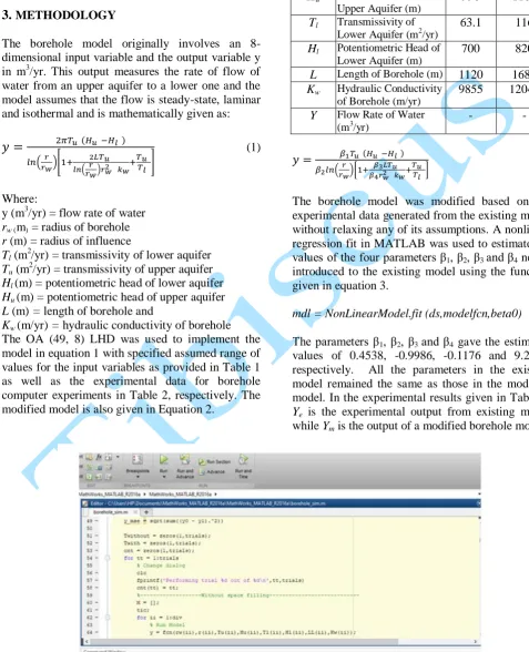
The borehole model was modified based on the experimental data generated from the existing model without relaxing any of its assumptions. A nonlinear regression fit in MATLAB was used to estimate the values of the four parameters β1, β2, β3 and β4 newly
introduced to the existing model using the function given in equation 3.
mdl = NonLinearModel.fit (ds,modelfcn,beta0) (3) The parameters β1, β2, β3 and β4 gave the estimated
values of 0.4538, -0.9986, -0.1176 and 9.2245, respectively. All the parameters in the existing model remained the same as those in the modified model. In the experimental results given in Table 2,
Table 2: Experimental data and outputs for borehole computer experiments using the existing and modified models
Run rw r Tu Hu Tl Hl L Kw Ye Ym
1 0.08 3218.25 64821.00 992.50 64.01 701.67 1126.51 10551.32 56.96 66.53
2 0.08 3219.62 64821.00 992.50 64.01 701.67 1126.51 10667.60 58.65 68.75
3 0.08 3220.99 64821.00 992.50 64.01 701.67 1126.51 10783.88 60.38 71.02
4 0.08 3222.36 64821.00 992.50 64.01 701.67 1126.51 10900.16 62.14 73.35
5 0.08 3223.73 64821.00 992.50 64.01 701.67 1126.51 11016.45 63.93 75.74
6 0.09 3225.11 64821.00 992.50 64.01 701.67 1126.51 11132.73 65.75 78.19
7 0.09 3226.48 64821.00 992.50 64.01 701.67 1126.51 11249.01 67.61 80.70
8 0.09 3219.82 64821.00 992.50 64.01 701.67 1126.51 10567.93 64.65 76.89
9 0.09 3221.19 64821.00 992.50 64.01 701.67 1126.51 10684.21 66.50 79.37
10 0.09 3222.56 64821.00 992.50 64.01 701.67 1126.51 10800.49 68.38 81.92
11 0.09 3223.93 64821.00 992.50 64.01 701.67 1126.51 10916.78 70.29 84.53
12 0.09 3225.30 64821.00 992.50 64.01 701.67 1126.51 11033.06 72.24 87.21
13 0.09 3226.67 64821.00 992.50 64.01 701.67 1126.51 11149.34 74.22 89.96
14 0.09 3218.44 64821.00 992.50 64.01 701.67 1126.51 11265.62 76.24 92.80
15 0.09 3221.38 64821.00 992.50 64.01 701.67 1126.51 10584.54 72.84 88.25
16 0.09 3222.75 64821.00 992.50 64.01 701.67 1126.51 10700.82 74.84 91.03
17 0.09 3224.13 64821.00 992.50 64.01 701.67 1126.51 10817.11 76.88 93.88
18 0.09 3225.50 64821.00 992.50 64.01 701.67 1126.51 10933.39 78.95 96.80
19 0.10 3226.87 64821.00 992.50 64.01 701.67 1126.51 11049.67 81.06 99.80
20 0.10 3218.64 64821.00 992.50 64.01 701.67 1126.51 11165.95 83.20 102.90
21 0.10 3220.01 64821.00 992.50 64.01 701.67 1126.51 11282.24 85.38 106.05
22 0.10 3222.95 64821.00 992.50 64.01 701.67 1126.51 10601.15 81.52 100.68
23 0.10 3224.32 64821.00 992.50 64.01 701.67 1126.51 10717.44 83.68 103.78
24 0.10 3225.69 64821.00 992.50 64.01 701.67 1126.51 10833.72 85.88 106.97
25 0.10 3227.07 64821.00 992.50 64.01 701.67 1126.51 10950.00 88.12 110.23
26 0.10 3218.84 64821.00 992.50 64.01 701.67 1126.51 11066.28 90.39 113.61
27 0.10 3220.21 64821.00 992.50 64.01 701.67 1126.51 11182.56 92.70 117.04
28 0.10 3221.58 64821.00 992.50 64.01 701.67 1126.51 11298.85 95.05 120.55
29 0.10 3224.52 64821.00 992.50 64.01 701.67 1126.51 10617.76 90.69 114.26
30 0.10 3225.89 64821.00 992.50 64.01 701.67 1126.51 10734.05 93.02 117.73
31 0.10 3227.26 64821.00 992.50 64.01 701.67 1126.51 10850.33 95.38 121.28
32 0.11 3219.03 64821.00 992.50 64.01 701.67 1126.51 10966.61 97.79 124.95
33 0.11 3220.40 64821.00 992.50 64.01 701.67 1126.51 11082.89 100.24 128.68
34 0.11 3221.77 64821.00 992.50 64.01 701.67 1126.51 11199.18 102.72 132.50
35 0.11 3223.15 64821.00 992.50 64.01 701.67 1126.51 11315.46 105.24 136.42
36 0.11 3226.09 64821.00 992.50 64.01 701.67 1126.51 10634.38 100.35 129.09
37 0.11 3227.46 64821.00 992.50 64.01 701.67 1126.51 10750.66 102.85 132.95
38 0.11 3219.23 64821.00 992.50 64.01 701.67 1126.51 10866.94 105.39 136.94
39 0.11 3220.60 64821.00 992.50 64.01 701.67 1126.51 10983.22 107.97 140.99
40 0.11 3221.97 64821.00 992.50 64.01 701.67 1126.51 11099.51 110.59 145.14
41 0.11 3223.34 64821.00 992.50 64.01 701.67 1126.51 11215.79 113.25 149.40
42 0.11 3224.71 64821.00 992.50 64.01 701.67 1126.51 11332.07 115.95 153.77
43 0.11 3227.65 64821.00 992.50 64.01 701.67 1126.51 10650.99 110.51 145.27
44 0.11 3219.42 64821.00 992.50 64.01 701.67 1126.51 10767.27 113.18 149.60
45 0.12 3220.80 64821.00 992.50 64.01 701.67 1126.51 10883.55 115.90 154.00
46 0.12 3222.17 64821.00 992.50 64.01 701.67 1126.51 10999.84 118.66 158.50
47 0.12 3223.54 64821.00 992.50 64.01 701.67 1126.51 11116.12 121.46 163.13
48 0.12 3224.91 64821.00 992.50 64.01 701.67 1126.51 11232.40 124.30 167.86
Figure 2: Representation of the output using the existing model and modified borehole model
The dotted line in Figure 1 represents the output of a modified borehole model while the thick line represents the output of an existing borehole model.
4. CONCLUSION
This study presents a technique for modifying a borehole model to develop a borehole computer experiment using orthogonal array-based Latin hypercube design (OALHD) with 49 runs and 8 input variables. Both the standard and a modified model are used with specified ranges of values for the borehole variables. The two models were used to compare their output which is the flow rate of water and see how close or accurate the output from a modified borehole model is relative to the output of the standard model. The modified model has performed well in developing a borehole computer experiment following the results obtained in this study which are close to those of the standard model. This study concludes that a modified borehole model can be used to develop a borehole computer experiment.
REFERENCES
[AO01] An J., Owen A. B. – Quasi-regression, Journal of Complexity, vol. 17: 588-607, 2001.
[C+02] Chen T. Y., Zwick J., Tripathy B., Novak G. – 3D engine analysis and mls cylinder head gaskets design.
Society of Automotive Engineers, SAE
[FW94] Fang K. T., Wang Y. –
Number-Theoretic Methods in Statistics,
Chapman and Hall, London. 1994.
[FLS06] Fang K. T., Li R. Z., Sudjianto A. –
Design and modelling for computer experiments. Chapman and Hall/CRC, New York. 2006.
[GH14] Gramacy R. B., Haaland B. – Speeding up neighbourhood search in local Gaussian process prediction. Journal of Computational and Graphical Statistics; arXiv:1409.0074, 2014.
[HX00] Ho W. M., Xu Z. Q. – Applications of
uniform design to computer
experiments. Journal of Chinese
Statistical Association; vol. 38, 395-410, 2000.
[Li02] Li R. – Model selection for analysis of
uniform design and computer
experiment. International Journal of Reliability, Quality and Safety Engineering; vol. 9, 305-315, 2002.
[LZH00] Lo Y. K., Zhang W. J., Han M. X. –
Applications of the uniform design to quality engineering. Journal of Chinese Statistical Association; vol. 38, 411-428, 2000.
[MF83] Miller D., Frenklach M. – Sensitivity analysis and parameter estimationin dynamic modelling of chemical kinetics.
International Journal of Chemical Kinetics; vol. 15, 677-696, 1983.
[MMY93] Morris M. D., Mitchell T. J., Ylvisaker D. – Bayesian design and analysis of computer experiments: Use of derivatives in surface prediction. Technometrics; vol. 35, 243-255, 1993. [OYA15] Osuolale K. A., Yahya W. B.,
Adeleke B. L. – Construction of
orthogonal array-based Latin
hypercube designs for deterministic
computer experiments. Annals.
experiment. International Journal of Advanced Science and Technology; 107(2), 21-32, 2017.
[Q+06] Qian Z., Seepersad C., Joseph R., Allen J., Wu C. F. J. – Building surrogate models based on detailed and
approximate simulations. ASME
Transactions, Journal of Mechanical Design; vol. 128, 668-677, 2006.
[SSW89] Sacks J., Schiller S. B., Welch W. J. –
Designs for computer experiments.
Technometrics; vol. 31, 41-47, 1989.
[S+89] Sacks J., Welch W. J., Mitchell T. J., Wynn H. P. – Design and analysis of
computer experiments. Statistical
Science; vol. 4(4), 409-423, 1989.