High performance of the support vector machine in classifying hyperspectral data using a limited dataset

(1)

IJMGE

Int. J. Min. & Geo-Eng.

Vol.49, No.2, December 2015, pp.253-268

High performance of the support vector machine in classifying

hyperspectral data using a limited dataset

Amir Salimi

1*

, Mansour Ziaii

1

, Mahdieh Hosseinjani Zadeh

2

, Ali Amiri

3

and Sadegh

Karimpouli

4

1. Faculty of Mining, Petroleum and Geophysics, Shahrood University of Technology, Shahrood, Iran

2. Department of Ecology, Institute of Science and High Technology and Environmental Science, Graduate University of

Advanced Technology, Kerman, Iran

3. Computer Engineering Group, Faculty of Engineering, Zanjan University, Zanjan, Iran

4. Mining Engineering Group, Faculty of Engineering, Zanjan University, Zanjan, Iran

Received 2 Feb. 2014; Received in revised form 24 Oct. 2015; Accepted 5 Dec. 2015

_{Corresponding author Email address: [email protected], Fax: +98 2332395509, Tel: +98 9122423908}

Abstract

To prospect mineral deposits at regional scale, recognition and classification of hydrothermal alteration zones using remote sensing data is a popular strategy. Due to the large number of spectral bands, classification of the hyperspectral data may be negatively affected by the Hughes phenomenon. A practical way to handle the Hughes problem is preparing a lot of training samples until the size of the training set is adequate and comparable with the number of the spectral bands. In order to gather adequate ground truth instances as training samples, a time-consuming and costly ground survey operation is needed. In this situation that preparing enough field samples is not an easy task, using an appropriate classifier which can properly work with a limited training dataset is highly desirable. Among the supervised classification methods, the Support Vector Machine is known as a promising classifier that can produce acceptable results even with limited training data. Here, this capability is evaluated when the SVM is used to classify the alteration zones of Darrehzar district. For this purpose, only 12 sampled instances from the study area are utilized to classify Hyperion hyperspectral data with 165 useable spectral bands. Results demonstrate that if parameters of the SVM, namely C and σ, are accurately adjusted, the SVM can be successfully used to identify alteration zones when field data samples are not available enough.

(2)

1. Introduction

Classification is defined as a process which converts data into meaningful information [26]. Supervised classification, a powerful type of classification is based on a set of labeled data which are named training samples. The training samples enable supervised classification methods to understand classification rules by means of several features as explanatory variables. The features are all sorts of information about unknown patterns that should be gathered in order to train classifiers. Nowadays, large-sized datasets with tens, hundreds, or thousands of features are easily available because of the improvements in data acquisition technology, the low costs of data storage, and the development of database technology. On the other hand, with high dimensional datasets, the size of the search space increases and the generalization capacity of classification decreases [14].

The supervised classification is commonly used for the analysis of remote sensing data. The remote sensing data with valuable information about the composing materials of the earth surface, allows characterization, identification, and classification of the surface objects. With the recent developments of sensor technology, hyperspectral sensors have been produced that can acquire remote sensing images in hundreds of spectral channels. Hyperspectral sensors collect a vast amount of spectral information about land surface objects in numerous narrow and continuous spectral bands. In comparison with multispectral sensors which collect spectral information in a few wide non-contiguous bands, hyperspectral sensors expand the capabilities of the multispectral kind by preparing more information about the spectral signature of land cover classes [7]. Although the high spectral resolution nature of hyperspectral images is an important advantage, their analysis is more difficult than multispectral ones. The curse of dimensionality, high spectral redundancy, noise, and nonlinear relations between spectral channels and corresponding materials are common problems of hyperspectral data analysis [30, 10, 5]. Because of these reasons, the classification of hyperspectral data is a very challenging problem. The efficiency of classification may be compromised when the appropriate methods for multispectral images

classification are utilized for hyperspectral data [5]. Therefore, to consider the special characteristics of the hyperspectral data, specific classification and segmentation methods should be utilized [33].

It should be noted that the curse of dimensionality is an important problem of the hyperspectral data classification. This problem arises from the spectral domain where each pixel of the hyperspectral images is represented by a vector of electromagnetic wavelengths measured by sensors which are named spectral bands. The size of the vector is equal to the number of spectral bands [7]. As mentioned previously, several hundreds of spectral bands are typically available for hyperspectral images in comparison to up to ten bands of the multispectral images [10]. Although the large number of spectral bands in hyperspectral data can increase the accuracy rate of classification, the absence of adequate training samples can degrade its performance. This problem results from insufficient training samples compared to the size of the feature space (or spectral band space). In other words, because of the high dimensionality of the feature space, the training data in this space look sparse and empty [33]. The degraded accuracy in consequence of the curse of dimensionality is known as an ill-posed problem and named the Hughes phenomenon [38, 33, 30, 1, 10]. Hughes theoretically demonstrated the relations between the number of the training samples, dimension of feature space, and classification accuracy [23]. Figure 1 represents the Hughes phenomenon where the average accuracy of classification has been shown as a function of the feature space dimension or measurement complexity. In addition, the parameter (m) of each curve shows the number of the available training samples.

(3)

Salimi et al./ Int. J. Min. & Geo-Eng., Vol.49, No.2, December 2015

For example, Maximum Likelihood Classifier (MLC), a widely used traditional parametric method, requires a specific number of training pixels (at least, m= number of features + 1) to have a reliable estimation of class parameters [38]. Undoubtedly, in some fields, preparing training samples with the mentioned size for a high dimensional dataset classification is a very difficult task. Consequently, obtaining enough training samples is a main challenge in the supervised classification of hyperspectral data

[7]. However, in most applications like mineral deposit prospecting, due to the lack of access to the prospected area and the expensive and time-consuming process of ground-truth data gathering especially in remote study regions [11, 7, 38, 30, 26, 24], the number of collected instances as training samples is not sufficient for a proper learning of classifier. As a result, undesirable occurrences like the Hughes phenomenon, over-fitting, and poor generalization are expected [7].

Fig. 1. The mean recognition accuracy versus measurement complexity with finite training samples (Modified from [23])

A promising choice for hyperspectral data classification that covers the mentioned problem is using supervised kernel-based methods [7, 38, 30, 26, 6]. The kernel-based classifiers solve a linear problem after mapping data from the original input space to a higher dimension feature space. Among the most widely used kernel-based methods for hyperspectral data classification, the Support Vector Machine (SVM) has outperformed results with respect to other ones. The SVM as a popular classifier has been extensively applied for classification of the hyperspectral images by widespread scientific fields [5, 3, 33, 28, 40]. Due to its intrinsic characteristics, the SVM has a high capability to classify problems which have limited numbers of training samples [7, 5]. Unlike traditional parametric methods which are based on the statistical parameters estimation of data, the SVM utilizes structural risk minimization without having any prior knowledge or assumption about data probability distribution [30, 26].

Similar to different sciences, remote sensing data are also utilized by extensive fields of geological sciences, such as environmental geology and mineral and hydrocarbon exploration. Mineral mapping as an important step of ore mineral prospecting has been successfully performed by this technology. Hydrothermal alteration mineral mapping via remote sensing has been widely and successfully used for the exploration of various hydrothermal deposits [2, 16, 17, 18, 35, 36]. The high spectral resolution of hyperspectral data has greatly promoted the potential of hyperspectral remote sensing for mineral mapping and geological exploration [37], and in the last two decades, it has been an important tool for studying the minerals and rocks of the earth surface [41]. Hyperspectral sensors have also been utilized for obtaining accurate information about the hydrothermal alteration mineral assemblages [21, 13, 17].

(4)

spatial covering, limited availability, and relatively cost of the data acquisition process of airborne hyperspectral data, using space-borne data is inevitable [20]. By launching EO-1 in November 2000, the hyperspectral remote sensing from space became possible via the Hyperion sensor. The Hyperion with a single telescope and two spectrometers in VNIR and SWIR is composed of 242 spectral bands at 10 nm and 30 m spectral and spatial resolution, respectively. Although the Hyperion suffers from more noise compared to the airborne kinds [20], it has found various applications in consequence of providing useful data [7]. The high availability of the Hyperion data in comparison with the airborne data has provided unique opportunities to derive benefits from its valuable data. Many previous studies by various researchers have emphasized the importance of the Hyperion for hydrothermal alteration mineral mapping [22, 13, 4, 17].

Despite the feasibility of the SVM in hyperspectral image classification, less attention is paid to utilizing the SVM in Geosciences, especially for rock type and mineral mapping. Few publications are available for using the SVM in mineral classification [29, 38, 37]. Although these researchers have applied the SVM, they do not perform the sensitivity analysis of the SVM with respect to the Hughes problem. Therefore, the main aim of the present study is to evaluate whether the small amount of training samples affect the performance of the SVM. In order to reach this aim, the SVM was utilized for classification alteration zones when its training step was done by only 12 training instances sampled from the study area. Darrehzar copper porphyry type deposit and its adjacent regions were selected as the study area of this research, as well.

The remaining sections of the paper have been organized as follows: Geological and geographical characteristics of the study area are introduced in section 2. Detailed descriptions about the utilized materials, including available datasets (the Hyperion scene and field samples) and methods (the SVM and error estimators) are stated in section 3. The results are reported in section 4 and finally, the conclusion is stated in section 5.

2. Study area

The study area is located in the Iranian

Uromiyeh-Dokhtar magmatic belt. This belt in Iran has been formed by diagonal stretching and the subduction of the Arabian plate beneath central Iran. It contains extensive porphyry copper type mineralization, including important mines like Sarcheshmeh, Sungon, and Meydouk [39]. The Darrehzar porphyry copper mine, which is the study area of this paper, is located in the southern part of the mentioned magmatic belt and 8 km to the southeast of Sarcheshmeh (Fig. 2a, b).

The Darrehzar porphyry copper deposit has almost 67 Mt estimated ore mineral reserve with an average grade of 0.37% [27]. Eocene volcano-sedimentary rocks, composed of volcaniclastics, andesite, trachyandesite, and sedimentary rocks, have hosted mineralized Oligocene-Miocene diorite and granodiorite formations (Fig. 2c) that have both been extensively altered by hydrothermal fluids into potassic, phyllic, propylitic, and argillic products. In addition, in consequence of supergene processes and the leaching of sulfides, large amounts of reddish or yellowish color oxidation products were produced [12]. The alteration zones are relatively oval shaped with the length of about 2.2 km and the width of 0.7–1 km, whereas the extensive phyllic and propylitic zones as well as the less extensive argillic zone are seen in the area [34]. However, no potassic alteration is seen at the surface [12].

3. Material and Methods

3.1. Hyperion dataset

(5)

Fig. 2. (a) Location of the study area in Iran, (b) Geological map of the study area at a small scale, (Modified from [17]), (c) Geological map of the study area at a large scale (Modified from [34])

(6)

Before the utilization of the Hyperion, it is essential to implement some pre-processing steps on the dataset, because the noisy nature of the Hyperion should be considered by correction of abnormal pixels, striping, and smile. In what follows, the main pre-processing algorithms implemented on the dataset have been briefly explained.

First, non-calibrated plus overlay bands were eliminated. Then, the de-striping algorithm was applied to reduce the stripe, especially in the first 12 VNIR and many SWIR bands. Although the de-striping algorithm decreases noise effects, some bands still comprise excessive noises, including the abnormal pixels with negative digital numbers (DN) and pixels with constant and intermediate DN values. In order to identify the remaining abnormal pixels and stripes, the visual manner was used, because it is a possible and an easy task.

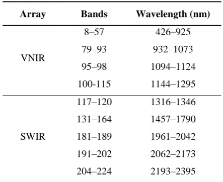
To eliminate atmospheric effects, FLAASH algorithm (The Fast Line-of-sight Atmospheric Analysis of Spectral Hyper-cubes) was utilized. Finally, after the elimination of water vapor relevant to absorption bands (i.e. bands 121–130 and 165–180), 165 remaining bands were applied as the main dataset, according to Table 1.

Table 1. List of the 165 bands of the Hyperion as the useable dataset after pre-processing

Array Bands Wavelength (nm)

VNIR

8–57 79–93 95–98 100-115

426–925 932–1073 1094–1124 1144–1295

SWIR

117–120 131–164 181–189 191–202 204–224

1316–1346 1457–1790 1961–2042 2062–2173 2193–2395

3.2. Field samples as training dataset

Supervised classification methods need training samples to learn the discriminative

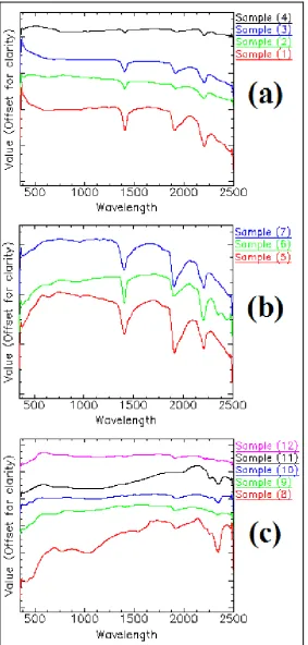
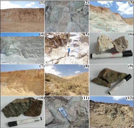
rules of patterns properly. In this research, the training dataset was selected from samples which were gathered at the study area. To evaluate the robustness of the SVM regarding the small size of the training set, the collection of a small number of the field samples has been attempted. Therefore, 12 rock samples of the alteration zones were collected and spectrally measured by Analytical Spectral Devices (ASD) FieldSpc3 at the Department of Ecology, Institute of Science and High Technology and Environmental Science, Graduate University of Advanced Technology, Kerman, Iran. The output of the ASD was analyzed by an automated mineral identification program, namely PIMA View, to see the semi-quantitative abundance of some alteration minerals. The alteration type of each sample was determined by expert opinion and the PIMA View results. Phyllic and weak phyllic zones were discriminated by the abundance value of muscovite and illite, the two indicator minerals of the phyllic alteration zone. Therefore, among the seven non-propylitic samples, four samples are assigned to the class phyllic and three samples to the class weak phyllic. As can be seen in Figure 4 which displays the Hyperion image spectrums of these seven samples, most of the phyllic samples show higher reflectance in comparison with the weak phyllic samples. The spatial, spectral, visual, and descriptive specifications of the 12 samples are summarized in Table 2 and Figures 5-7.

Fig. 4. Hyperion image spectrums of the seven field samples of the phyllic zone. Red: 4 phyllic

(7)

Table 2. The spatial, spectral, visual, and descriptive specifications of the 12 field samples

No.

Specifications

Spatial Spectral Visual

Descriptive

Alteration type PIMA View output Muscovite & Illite

1 393937 E

3306057 N Fig. 6a Fig. 7 (1) Phyllic >60 %

2 393958 E

3 394156 E

4 394418 E

5 393625 E

3305920 N Fig. 6b Fig. 7 (5) Weak phyllic < 30 %

6 393881 E

3305702 N Fig. 6b Fig. 7 (6) Weak phyllic <30 %

7 394656 E

3306319 N Fig. 6b Fig. 7 (7) Weak phyllic < 30 %

8 393880 E

3305612 N Fig. 6c Fig. 7 (8) Propylitic -

9 394743 E

10 394769 E

11 394048 E

12 393106 E

(8)

(9)

Fig. 7. Visual characteristics of the 12 field samples

3.3. Support vector machine (SVM)

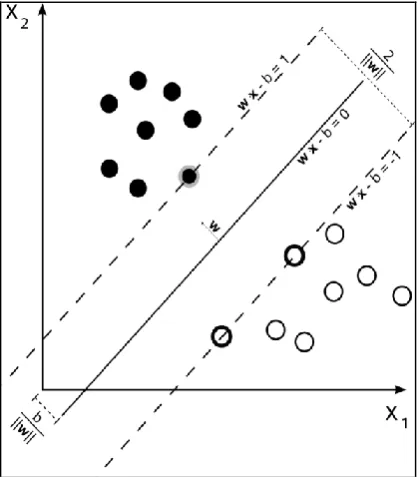
Support Vector Machine (SVM) [8], a supervised non-parametric statistical learning-based classification technique [26], has been widely used for the classification of hyperspectral data recently [31]. Classification by the SVM is based on structural risk minimization, whereas an optimal hyperplane maximizes distance between the margins of two classes by the application of a small number of training samples, called Support Vectors (SV). The SVM is not greatly affected by limited training samples, because the SV samples are merely used for the classification process [8]. Although in its simplest mode, the SVM is a linear binary classifier (Fig. 8), it can be extended to more than two classes by

splitting the problem into a series of binary class separations, then one of the two widely applied techniques for multiclass classification, namely One-Against-One (OAO) and One-Against-All (OAA) [7] can be used. Practically, data points of different classes usually overlap with one another and linear SVM cannot classify these situations accurately [26]. This problem is solved by the soft margin SVM and the kernel-based SVM in order to represent more complex shapes than linear hyperplanes [7]. Basics of the SVM formulations are reviewed as follows:

For a given training set







i i



(10)

samples. While the data in the feature space are linearly separable, the standard linear binary SVM can classify the data by means of the hyperplane f X

 

W.X b 0 and maximum geometric margin

2

2 W

. Therefore,

the objective of the SVM is solving the following quadratic optimization problem with proper inequality constraints:

Fig. 8. Binary SVM in the simplest mode





2

1 min

2

. 1 1, ,

i i

y b i n

                W W X (1)

Due to the indirect effect of inequality constraints on the main optimization problem, by introducing the Lagrange multipliers (α), the following alternative dual representation is resulted.





1 1 1

1

, 2

0, 1

0

n n n

i i j i j i j

i i j

i n

i i i

max y y

i n y             _                   







X X (2)

The dual optimization problem is solved with respect to (α) by considering the following KKT conditions.

















, , 0 , , 0

0, 1

. 1 0

[ . 1] 0

i

i i

i i i

L b L b b i n y b y b                               W α W W α W X W X (3)

The above equations are well known as the hard margin SVM, where the members of the two classes are completely linear separated. In the non-separable cases, the generalization capacity of the SVM can be increased by introducing slack variables (ξ) and the associated penalization parameter (C). As a result, the soft margin SVM with soft constraint equations is defined thus:





2

1

min C ξ

2

. 1 ξ 1, ,

ξ 0

n i i

i i i

i

y b i n

  _                     



W

W X (4)

The dual mode optimization problems of (2) and (4) are solved with some quadratic optimization techniques and are calculated and then W and b can be obtained. Finally, the class label for any given sample is predicted by:

 



.



f x sgn W X b (5)

The SVM utilizes just SV samples with nonzero Lagrange multipliers (α) to define the separation hyperplane, and the remaining samples of the training dataset do not contribute to the training process. For this reason, the SVM is known as a robust method for the classification of limited datasets.

(11)

Fig. 9. Nonlinear transformation of the input space to construct separating hyperplane in another high dimension space (Hilbert space) by the nonlinear mapping function, ϕ (b) [6]

3.4. Error estimation methods

In order to assess the performance and reliability of a designed classifier, its actual error should be measured. Practically, it is not possible to measure the exact value of the actual error, because the underlying feature-label distribution of real problems is unknown. Therefore, an approximate value of the actual error is estimated by error estimation methods and the available dataset [42]. Usually, the available dataset is divided into training and test sets, where the former is utilized to train the classifier and adjust its parameters and the latter is applied to validate it [9]. The size of the dataset is an effective factor for selecting a consistent error estimation method among available error estimators. Clearly speaking, when a large amount of data is available, a certain amount of it is reserved for testing and the remainder is utilized for training, without any overlapping between training and test sets. The Holdout method is a kind of error estimator which implements the above procedure on the large-sized data sets. On the other hand, in some real-world fields, there are no adequate numbers of data samples to allow some of them to be kept back for testing. This problem poses significant challenges in the application of the Holdout error estimator and requests other estimation methods for small-sized datasets, such as re-substitution, k-fold cross-validation, Leave-One-Out cross-validation, etc. [42].

In the re-substitution method, the whole sample set is used for designing and again for testing the classifier. Since the train and test sets are exactly the same, the results of the re-substitution method are optimistically biased

[15]. The dataset used by the k-fold cross-validation should be split into nearly k equal size subsets. At the k-iterations, one of the subsets is selected as the test set and the rest k-1 form the training set. The classifier trained by the training set is used to estimate the error on the test set. Finally, an average of the k obtained errors is considered as the error of the classifier. The Leave-One-Out cross-validation is a complete kind of the k-fold cross-validation in which k equals the size of the dataset [25].

4. Results and Discussion

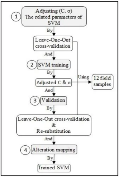
The SVM-based classification of the alteration zones was done in 4 steps according to the flowchart of Figure 10. Before starting the first step of the flowchart, a few points need to be explained:

Number of alteration classes: Based on the alteration type column of Table 2, three different types of alteration were supposed, including Phyllic, weak Phyllic, and Propylitic.

Normalized data: To prevent biased results, classification should be done by the normalized dataset.

Multi-class SVM: Because the SVM in the initial form is a binary classification method, the One-Against-One (OAO) procedure was used to combine binary results and perform multi-classification.

(12)

Fig. 10. Flowchart of the SVM-based classification process

Considering the above points, the details of the 4 steps of classification flowchart are explained:

Step 1. In the first step, it is necessary to adjust the parameters of the SVM, namely C and σ. It should be noted that incorrect estimation of these parameters can negatively affect the final results of classification. To set the mentioned parameters, the Leave-One-Out cross-validation technique, appropriate for limited datasets, was utilized. The cross-validation was implemented by varied values of σ (i.e. 0.001, 0.005, 0.01, 0.05, 0.1, 0.5, and 1) and C (100 to 2000 by an interval step of 100), and the mean accuracy of classification by each pair value of σ and C was calculated. The obtained results of cross-validation have been shown in Table 3, where the corresponding values of maximum accuracy are the optimum values. As can be seen, the maximum value of accuracy (76.92%) has been obtained by σ≥ 0.5 and a wide range of C.

Table 3. Results of Leave-One-Out cross-validation to obtain the best values of SVM parameters

σ C Mean accuracy (%)

≤ 0.001 100-2000 23.08

0.005 100-2000 46.15

0.01 100-2000 46.15

0.05 100-2000 53.85

0.1

100 69.23

200 61.54

300-2000 53.85

≥ 0.5 100-2000 76.92

Step 2. The optimum values of C and σ in the previous step were utilized to train the SVM. Because of the extensive range of C as well as its low effect on the classification result, only two values in the beginning and the end of the range were selected. Therefore, the classification process will be done by two pairs of σ and C, including (0.5, 100), (0.5, 2000).

Step 3. It is obvious that by the implementation of the Leave-One-Out cross-validation at step 1, the cross-validation has been previously done and the average accuracy equal to 76.92% has been obtained. Now, another validation technique, namely re-substitution, is applied which is appropriate for the error estimation of the small-sized datasets. According to 4, the results of validation have been presented by means of overall accuracy, average accuracy, and the kappa value.

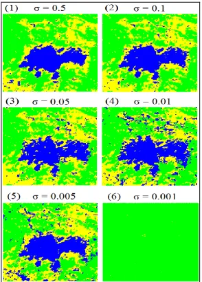
Step 4. The SVM trained by the optimum parameters of step 2 was used to map the alteration zones of the study area (Fig. 11). To observe the effect of using incorrect parameters on the classification result, alteration maps resulted from non-optimum σ were displayed in Figure 12, as well. It can be seen that the various values of σ have produced alteration maps with different accuracies. For example, most of the area of the alteration map resulted from σ= 0.001 has been covered by the propylitic zone inaccurately (Figs. 12, 6). According to 3, the lowest accuracy (23.08%) was obtained by Leave-One-Out cross-validation for σ= 0.001.

Table 4. The obtained accuracy of the SVM by the optimum values of C and σ using the re-substitution error estimator and 12 field samples

SVM parameters Accuracy

σ C Overall accuracy (%) Average accuracy (%) Kappa value

0.5 100-2000 83.33 80.56 0.7624

Table

(13)

Fig. 11. Final classified alteration maps resulted from the SVM by (a) σ= 0.5, C= 100 and (b) σ= 0.5, C= 2000

(14)

5. Summary and Conclusions

The supervised classification techniques need ground truth data to be trained in the training phase of classification. Due to the large number of spectral bands of hyperspectral data, it is necessary to prepare a lot of samples as training set for hyperspectral classification. A confident way of gathering a reliable training set is ground survey in the study area. This task needs a relatively long time for sampling and a high cost for analysis. Sampling can be more problematic, especially in prospecting areas with low accessibility which means adequate training samples are not usually prepared. Therefore, a classification method which is consistent with small-sized datasets is highly required. The important and discriminative advantage of the SVM is its high ability to classify problems in which ground truth data are not available enough for the training step of classification. To evaluate this capability, a low number of the rock samples, namely 12, sampled from the study area were utilized to train the SVM. An accurate estimation of SVM parameters can increase the generalization and reliability of classification results. If these parameters are not correctly adjusted, it can strongly affect the accuracy rate of classification. Therefore, to set most optimum values of C and σ, the Leave-One-Out cross-validation method was applied. Finally, the SVM trained by the obtained parameters and the 12 available field samples was utilized to map the alteration zones of the study area. The acceptable results of classification confirm that the SVM is the best choice that can be used by fields in which adequate ground truth data collection is difficult because of various reasons, such as the lack of availability of remotely sensed areas and the time-consuming and costly nature of the data gathering task.

References

[1] Alajlan, N., Bazi, Y., Melgani, F., Yager, R. (2012). Fusion of supervised and unsupervised learning for improved classification of hyperspectral images. Journal of Information

Sciences 217, 39-55. Doi:

10.1016/j.ins.2012.06.031

[2] Amer, R., Kusky, T., El Mezayen, A. (2012). Remote sensing detection of gold related alteration zones of Um Rus Area, Central Eastern

Desert of Egypt. Advances in Space Research, 49(1), 121-134. Doi:10.1016/j.asr.2011.09.024

[3] Bazi, Y. and Melgani, F. (2006). Toward an optimal SVM classification for hyperspectral remote sensing images. IEEE Transactions on Geoscience and Remote Sensing, 44(11), 3374-3385. Doi: 10.1109/TGRS.2006.880628

[4] Bishop, C.A., Liu, J.G., Mason, P.J. (2011). Hyperspectral remote sensing for mineral exploration in Pulang, Yunnan Province, China. International Journal of Remote Sensing, 32(7), 2409-2426. Doi: 10.1080/01431161003698336 [5] Camps-Valls, G., Gomez-Chova, L., Calpe-Maravilla, J., Martin-Guerrero, J.D., Soria-Olivas, E., Alonso-Chorda, L., Moreno, J. (2004). Robust support vector method for hyperspectral data classification and knowledge discovery. IEEE Transactions on Geoscience and Remote Sensing, 42, 1530-1542. Doi: 10.1109/TGRS.2004.827262

[6] Camps-Valls, G., Tuia, D., Bruzzone, L., Benediktsson, J. (2014). Advances in Hyperspectral Image Classification. IEEE Signal Processing Magazine, 31(1), 45-54. Doi: 10.1109/MSP.2013.2279179

[7] Chang, C. (2007). Hyperspectral Data Exploitation, Theory and Applications. Published by John Wiley & Sons, Inc., Hoboken, New Jersey.

[8] Cortes, C. and Vapnik, V. (1995). Support-vector Networks. Machine Learning, 20(3), 273-297.

[10] Fauvel, M., Tarabalka, Y., Benediktsson, J.A., Chanussot, J., Tilton, J.C. (2013). Advances in Spectral-Spatial Classification of Hyperspectral Images. Proceedings of the IEEE, 101(3), 652-675. Doi: 10.1109/JPROC.2012.2197589

[11] Foody, G.M. and Mathur, A. (2004b). Toward intelligent training of supervised image classifications: directing training data acquisition for SVM classification. Remote Sensing of Environment, 93(1-2): 107-117.

Doi: 10.1016/j.rse.2004.06.017

[12] Geological survey of Iran. (1973a). Exploration for Ore deposits in Kerman region. Report No, Yu/53. Tehran, Iran: Ministry of Economy Geological Survey of Iran.

(15)

sensor, northern Danakil, Eritrea. International Journal of Remote Sensing, 29(13), 3911-3936.

Doi: 10.1080/01431160701874587

[14] Gheyas, A., Leslie, S.S. (2010). Feature subset selection in large dimensionality domains, Pattern Recognition, 43, 5-13. Doi: 10.1016/j.patcog.2009.06.009

[15] Heikkila, J.(1992). ESTIMATION OF

CLASSIFIER'S PERFORMANCE WITH

ERROR COUNTING, XVIIth ISPRS

Congress, Technical Commission III: Mathematical Analysis of Data, Washington, D.C., USA, August 2-14,325-334.

[16] Hosseinjani Zadeh, M., Tangestani, M.H. (2011). Mapping alteration minerals using sub-pixel unmixing of ASTER data in the Sarduiyeh area, southeastern Kerman Iran. International Journal of Digital Earth, 4(6), 487-504. Doi: 10.1080/17538947.2010.550937

[17] Hosseinjani Zadeh, M., Tangestani, M.H., Velasco Roldan, F., Yusta, I. (2014a). Sub-pixel mineral mapping of a porphyry copper belt using EO-1 Hyperion data. Advances in Space Research, 53(3), 440-451. Doi: 10.1016/j.asr.2013.11.029

[18] Hosseinjani Zadeh, M., Tangestani, M.H., Velasco Roldan, F., Yusta, I. (2014b). Mineral exploration and alteration zone mapping using mixture tuned matched filtering approach on ASTER data at the central part of Dehaj-Sarduiyeh copper belt, SE Iran. IEEE selected topics in applied earth observations and remote

sensing. 7(1),284-289.Doi:

10.1109/JSTARS.2013.2261800

[19] Huang, C., Song, K., Kim, S., Townshend, J.R.G., Davis, P., Masek, J.G., Goward, S.N. (2008). Use of dark object concept and support vector machines to automate forest cover change analysis. Remote Sensing of Environment, 112(3), 970-985. Doi: 10.1016/j.rse.2007.07.023

[20] Kruse, F.A. (2003). Mineral Mapping with AVIRIS and EO-1 Hyperion. Presented at the 12th JPL Airborne Geoscience Workshop, Pasadena, California.

[21] Kruse, JW. and Boardman, F.A. (2000). Characterization and Mapping of Kimberlites and Related Diatremes Using Hyperspectral Remote Sensing. IEEE Aerospace Conference

Proceedings, 3, 18-24. Doi:

10.1109/AERO.2000.879859

[22] Kruse, F.A., Boardman, J.W., Huntigton, J.F. (2003). Comparison of airborne Hyperspectral data and EO-1 Hyperion for mineral mapping.

IEEE Transactions on Geoscience and Remote Sensing, 41(6), 1388-1400. Doi: 10.1109/TGRS.2003.812908

[23] Landgrebe, D.A. (2002). Hyperspectral Image Data Analysis. IEEE Signal processing Magazine, 19(1), 17-28. Doi: 10.1109/79.974718

[24] Li, J. and Bioucas-Dias, J.M. (2013). Semi-supervised Hyperspectral Image Classification Using Soft Sparse Multinomial Logistic Regression. Geoscience and Remote Sensing Letters, IEEE, 10(2), 318-322. Doi: 10.1109/LGRS.2012.2205216

[25] Martin, G. K., Hirschberg, D. S. (1996). Small Sample Statistics for Classification Error Rates. Technical report, No, 96-21. Department of Information and Computer Science, University of California.

[26] Mountrakis, G., Im, J., Ogole, C. (2011). Support vector machines in remote sensing: A review. ISPRS Journal of Photogrammetry and

Remote Sensing, 66, 247-259.

Doi:10.1016/j.isprsjprs.2010.11.001

[27] NICICO. (2008). Darrehzar ore reserve estimates. Internal report of National Iranian Copper Industries Company.

[28] Okujeni, A., van der Linden, S., Tits, L., Somers, B., Hostert P. (2013). Support vector regression and synthetically mixed training data for quantifying urban land cover. Remote Sensing of Environment, 137, 184-197. Doi: 10.1016/j.rse.2013.06.007

[29] Oommen, T. (2008). An objective analysis of Support Vector Machine based classification for remote sensing, Mathematical Geosciences, 40(4), 409-424. Doi: 10.1007/s11004-008-9156-6

[30] Pal, M. and Foody, G.M. (2010). Feature Selection for Classification of Hyperspectral Data by SVM. IEEE Transactions on Geoscience and Remote Sensing, 48(5), 2297-2307. Doi: 10.1109/TGRS.2009.2039484

[31] Pal, M. and Mather, P.M. (2005). Support vector machines for classification in remote sensing. International Journal of Remote Sensing, 26(5), 1007-1011. Doi: 10.1080/01431160512331314083

(16)

[33] Plaza, A., Benediktsson, J.A., Boardman, J.W., Brazile, J., Bruzzone, L., Camps-Valls, G., Chanussot, J., Fauvel, M., Gamba, P., Gualtieri, A., Marconcini, M., Tilton, J.C., Trianni, G. (2009). Recent advances in techniques for hyperspectral image processing. Remote Sensing of Environment, 113, 110-122.

Doi: 10.1016/j.rse.2007.07.028

[34] Ranjbar, H., Hassanzadeh, H.,Torabi, M. (2001). Integration and analysis of airborne geophysical data of the Darrehzar area, Kerman Province, Iran, using principal component analysis. Journal of Applied Geophysics, 48(1), 33-41, Doi: 10.1016/S0926-9851(01)00059-3

[35] Shahriari, H., Honarmand, M., Ranjbar, H. (2015). Comparison of multi-temporal ASTER images for hydrothermal alteration mapping using a fractal-aided SAM method. International Journal of Remote Sensing, 36(5),

1271–1289. Doi:

10.1080/01431161.2015.1011352

[36] Shahriari, H; Ranjbar, H; Honarmand, M. (2013). Image Segmentation for Hydrothermal Alteration Mapping Using PCA and Concentration–Area Fractal Model. Natural Resources Research, 22(3), 191-206, Doi: 10.1007/s11053-013-9211-y

[37] Wang, Z.H. and Zheng, C.Y. (2010). Rocks/Minerals Information Extraction from EO-1 Hyperion Data Base on SVM.

International Conference on Intelligent Computation Technology and Automation, 3, 229-232. Doi: 10.1109/ICICTA.2010.341

[38] Waske, B., Benediktsson, J.A., Arnason, K., Sveinsson, J.R. (2009). Mapping of hyperspectral AVIRIS data using machine-learning algorithms. Canadian Journal of Remote Sensing, 35(1), 106-116.

[39] Waterman, G. and Hamilton, N. (1975). The Sarcheshmeh porphyry copper deposit. Economic Geology, 70, 568-576

[40] Yanfeng, G.u., Wang, S., Xiuping, J. (2013). Spectral Unmixing in Multiple-Kernel Hilbert Space for Hyperspectral Imagery. IEEE Transactions on Geoscience and Remote Sensing, 51(7), 3968-3981. Doi: 10.1109/TGRS.2012.2227757

[41] Zhang, X. and Peijun, L. (2014). Lithological mapping from hyperspectral data by improved use of spectral angle mapper. International Journal of Applied Earth Observation and Geoinformation, 31, 95-109. Doi: 10.1016/j.jag.2014.03.007