Earth Syst. Sci. Data, 5, 15–29, 2013 www.earth-syst-sci-data.net/5/15/2013/ doi:10.5194/essd-5-15-2013
©Author(s) 2013. CC Attribution 3.0 License.
History
ofGeo- and Space
Sciences
Open
Access
Advances
in Science & Research Open Access ProceedingsOpen
Access
Earth System
Science
Data
OpenAccess
Earth System
Science
Data
D
iscussions
Drinking Water
Engineering and ScienceOpen Access
Drinking Water
Engineering and ScienceDiscussions
O
pen
Acc
es
s
Social
Geography
Open
Access
D
iscussions
Social
Geography
Open
Access
Calibration procedures and first dataset of Southern
Ocean chlorophyll
a
profiles collected by elephant seals
equipped with a newly developed CTD-fluorescence tags
C. Guinet1, X. Xing2,3,4, E. Walker5, P. Monestiez5, S. Marchand6, B. Picard1, T. Jaud1, M. Authier1, C. Cott´e1,7, A. C. Dragon1, E. Diamond2,3, D. Antoine2,3, P. Lovell8, S. Blain9,10, F. D’Ortenzio2,3, and
H. Claustre2,3
1Centre d’Etudes Biologiques de Chiz´e-CNRS, Villiers en Bois, France 2Laboratoire d’Oc´eanographie de Villefranche, Villefranche-sur-Mer, France
3Universit´e Pierre et Marie Curie (Paris-6), Unit´e Mixte de Recherche 7093, Laboratoire d’Oc´eanographie de
Villefranche, Villefranche-sur-Mer, France
4Ocean University of China, Qingdao, China
5Unit´e Biostatistique et Processus Spatiaux-INRA, Avignon, France 6Mus´eum national d’histoire naturelle, DMPA USM 402/LOCEAN, Paris, France 7Universit´e Pierre et Marie Curie (Paris-6), DMPA USM 402/LOCEAN, Paris, France
8Sea Mammal Research Unit, University of St. Andrews, St. Andrews, Scotland 9Laboratoire d’Oc´eanographie Microbienne, Universit´e Paris VI, Banyuls sur mer, France
10Universit´e Pierre et Marie Curie (Paris-6), Unit´e Mixte de Recherche 7621, Laboratoire d’Oc´eanographie
Microbienne, Banyuls-sur-Mer, France
Correspondence to: C. Guinet (guinet@cebc.cnrs.fr)
Received: 21 June 2012 – Published in Earth Syst. Sci. Data Discuss.: 23 August 2012 Revised: 11 December 2012 – Accepted: 11 December 2012 – Published: 4 February 2013
Abstract. In situ observation of the marine environment has traditionally relied on ship-based platforms. The obvious consequence is that physical and biogeochemical properties have been dramatically undersampled, especially in the remote Southern Ocean (SO). The difficulty in obtaining in situ data represents the major lim-itations to our understanding, and interpretation of the coupling between physical forcing and the biogeochem-ical response. Southern elephant seals (Mirounga leonina) equipped with a new generation of oceanographic sensors can measure ocean structure in regions and seasons rarely observed with traditional oceanographic platforms. Over the last few years, seals have allowed for a considerable increase in temperature and salinity profiles from the SO, but we were still lacking information on the spatiotemporal variation of phytoplank-ton concentration. This information is critical to assess how the biological productivity of the SO, with direct consequences on the amount of CO2“fixed” by the biological pump, will respond to global warming. In this
16 C. Guinet et al.: Calibration procedures and first dataset of Southern Ocean chlorophyllaprofiles
1 Introduction
Polar marine ecosystems, and in particular the Southern Ocean (SO hereafter), are among the most vulnerable ecosys-tems to climate change. However, there is conflicting ev-idence on how the biological productivity of these Polar Oceans will respond to global warming. The SO plays an im-portant role in the carbon cycle and it is one of the largest sink for anthropogenic CO2through the formation of deep water
around Antarctica and intermediate water in the vicinity of the subantarctic zone (Caldeira et al., 2000; Lo Monaco et al., 2005). Furthermore, by contributing to roughly half of the biosphere’s primary production, photosynthesis by oceanic phytoplankton is a vital link between living and inorganic stocks of carbon (Field et al., 1998; Berhenfeld et al., 2006), but our current understanding of the variability of SO’s pri-mary productivity is hampered by the lack of in situ observa-tions available for this logistically difficult region, and much of the existing observations are heavily biased towards the austral summer.
Furthermore, the degree of confidence for primary produc-tion derived from satellite-based estimates of phytoplankton biomass is still debated. This is especially true in SO, where satellite measurements tend to under-estimate chlorophyll a (chl a hereafter) concentrations (Dierssen and Smith, 2000; Holm-Hansen et al., 2004; Garcia et al., 2005; Dierssen, 2010; Kahru and Mitchell, 2010). Satellites scan the sea sur-face and are unable to provide subsursur-face chlorophyll pro-files. Deep fluorescence maxima have been found within the frontal zone of the Antarctic Circum Current (ACC hereafter, Qu´eguiner and Brzezinski, 2002; Holm-Hansen et al., 2004) or in the vicinity of the ice edge (Waite and Nodder, 2001). Persistent cloud cover and fragmented sea-ice also constitute towards a major limitation of satellite ocean colour measure-ments in the SO (Arrigo et al., 1998; Buesseler et al., 2003). Evaluation of the distribution of chl a throughout the wa-ter column is one of the most important biological parame-ters in the ocean because it is an indicator of the spatial and temporal variability of primary productivity (Behrenfeld and Falkowski, 1997). The limitations of satellite assessments of primary production combined with a lack of primary pro-ductivity measurements in the field requires to complement remotely sensed ocean colour data with year-round surveys of the in situ optics as well as the physical oceanographic measurements for a description of spatial (horizontal and ver-tical) and temporal (seasonal, inter-annual) distribution of phytoplankton, but also give insights on its advection and fate. In turn, this data will contribute to our understanding of how primary production within SO may respond to climatic changes.
Subsurface chl a measurements are traditionally per-formed from research vessels, using profiling fluorometers and water samples collected by Niskin bottles. Alternatively, chl a profiles can be obtained from fluorometers deployed on fixed moorings or autonomous platforms like Argo floats
(Roemmich et al., 2004), or autonomous underwater vehi-cles (Yu et al., 2002). Rapid technological advances in ocean observation have nevertheless been achieved during the last decade, particularly with respect to physical climate vari-ables. Developing such in situ observation systems is an es-sential step towards a better understanding of biogeochemi-cal cycles and ecosystem dynamics, especially at spatial and temporal scales that have been unexplored until now. How-ever, with regard to the carbon cycle, the establishment of in situ observing systems in the under-sampled SO remains challenging due to its remoteness, harsh weather conditions and the presence of sea-ice.
Here we present the development of an original synergy between biologist’s efforts to understand the marine life of top predators, physical and biogeochemical oceanographic studies through development of new bio-logging devices de-ployed on southern elephant seals (Mirounga leonina), SES hereafter. This device incorporates high accuracy tempera-ture and salinity sensors, as well as a fluorometer and pro-vides a range of new behavioural and physiological data on free ranging marine animals for biologists, while simultane-ously gathering vertical profiles of temperature, salinity and fluorescence for oceanographers. Profiles sampled in the re-mote SO are of great interest as they can fill a niche within the ocean observing system, where such measurements are lacking (e.g., Charrassin et al., 2008; Nicholls et al., 2008; Roquet et al., 2009; Wunch et al., 2009). One important as-pect of this methodology is the near real-time delivery of CTD-Fluo profiles using the Argos satellite system (Argos, 1996). SESs provide an ideal “platform” for such investi-gation as they dive nearly continuously and at great depths (Hindell et al., 1991). Moreover, they undertake long forag-ing trips each year, explorforag-ing large areas of the SO (Biuw et al., 2007).
However, to make most of the use of these fluorescence data, it is essential to develop effective means for calibra-tion, quality control and postprocessing to provide a consis-tent dataset to oceanographers and for climatologies. There-fore, the first objective of this paper is to report the calibra-tion and the profile qualificacalibra-tion procedure on a unique 3-yr fluorescence dataset collected by SES within the Indian sector of the Southern Ocean. From this data, we will as-sess how in situ measurements compare with surface chl a concentration measured by ocean colour satellites. This new approach allows sustained acquisition of chl a fluorescence profiles (proxy for chl a concentration) in areas where data scarcity is the rule and how they complement satellite ocean colour data.
2 Materials and methods
2.1 Instrumentation
here (see also Fedak et al., 2002). CTD-Fluoro-SRDLs have been designed as miniaturised platforms to record be-havioural data and log in situ CTD profiles. They can be deployed on a range of marine mammals (e.g., Lydersen et al., 2002; Boehme et al., 2008; Nicholls et al., 2008; Roquet et al., 2009). The devices contain (1) a Platform Terminal Transmitter (PTT) to transmit compressed data through the Argos satellite system, (2) a micro-controller coordinates the different functions e.g., sensor data acquisition (data process-ing and transmission based on the internal setup and energy budget, Boehme et al. (2009) and (3) a miniaturised CTD (Valeport LTD, Totnes, UK).
The specifications of the miniaturised CTD (Valeport Ltd, Totnes, UK) result from a trade-off between the need for miniaturisation, energy consumption, stability and sensor performance. The pressure measurements are made by a Keller series-PA7 piezoresistive pressure transducer1 (Keller AG, CH) with a given accuracy of better than 1 % of the full-scale reading (±20 dbar at 2000 dbar). However, laboratory experiments have shown a performance of better than 0.25 % of the actual reading (Boehme et al., 2009). The temperature probe is a fast response Platinum Resistance Thermometer (PRT) made by Valeport (range:−5◦C to+35◦C, accuracy:
±0.005◦C, time constant: 0.7 s) and an inductive
conductiv-ity sensor by Valeport (range: 0 to 80 mS cm−1, accuracy: bet-ter than±0.01 mS cm−1).
Implementation of a fluorometer to estimate chlaconcentration
In vivo fluorescence F is a widely used technique to estimate chl a concentration in aquatic environments and can be ex-pressed as:
F=Ea∗[chl a]ϕf (1)
Where E (mole quanta m−2s−1) is the intensity of the
ex-citing source, a∗ is the chl-specific absorption coefficient
(m2mg [chl a]−1) where [chl a] is the chl a concentration
([chl-a] hereafter) (mg chl a m−3) andϕ
fis the quantum yield
for fluorescence [mole of emitted quanta (mole absorbed quanta−1)].
The fluorescence-chl a relationship for a given fluorom-eter varies according to environmental conditions such as the phytoplankton taxonomic composition and physiological adaptative mechanisms (e.g., Falkowski and Kolber, 1995; Babin et al., 1996, 2008).
The Cyclops 7 is a compact cylinder (110×25 mm after re-moval of the end cap), low energy consumption single chan-nel fuorescence detector that can be used for many different applications. It delivers a voltage output that is proportional to the concentration of the chl a particle, or compound of in-terest. For chl a detection a 460 nm exciting wavelength and a 620–715 nm fluorescence detection photodiode are used. According to Turner Design specifications the minimum de-tection limit is 0.025µg L−1 of chl a. The Cyclops 7 can be
set on a different level of sensitivity for chl a detection allow-ing detection of maximum chl a concentration rangallow-ing gener-ally from low (i.e., detection range 0–500µg L−1) to medium
(0–50µg L−1) and high (0–5µg L−1) sensitivities. For our
ap-plication according to chl a climatologies available, the ini-tial detection range was set between 0–2.5µg L−1, a range
well matching the chl a concentration generally encountered within the oceanic waters of the SO (Reynolds et al., 2001; Marrari et al., 2006; Uitz et al., 2009).
The Cyclops 7 was integrated in a new CTD-Fluo Satel-lite Relay Data Loggers (Tags hereafter). They were built by the Sea Mammal Research Unit (SMRU) (University of St. Andrews, Scotland). Fluorescence was sampled contin-uously between the surface and 180 m. As Argos messages are restricted in length, we had to reduce the resolution of fluorescence data. Therefore, values were averaged for eigh-teen 10 m vertical sections. For each section the mean fluo-rescence value was allocated to the mid-depth point of the corresponding section.
Fluorometer calibrations, relying essentially on chl a so-lutions or on phytoplankton cultures, are generally provided by manufacturers. Most of the time these calibrations are es-tablished for large range of chl a concentrations not always representative of in situ ones. Therefore, it is highly desir-able to confirm or adjust through in situ calibration on natural samples (see Xing et al., 2012). As part of this programme, a thorough calibration and testing procedure was undertaken for the CTD-Fluo SRDL. Pre-deployment calibrations of the tags and at-sea validating tests were conducted prior to SES deployment. This procedure was followed for most deploy-ments in this study. Before being taken into the field, devices were calibrated at Valeport, Service Hydrographique de la Marine (Brest, France), and had temperature (T ) and con-ductivity (C) resolutions of 0.001◦C and 0.002 mS cm−1,
re-spectively (see Roquet et al., 2011 for details).
2.2 Calibration procedure
The fluoremeters were inter-calibrated by implementing a Bayesian procedure using all information available regarding predeployment tests as well as post-deployment information collected.
2.2.1 Fluorometer inter-calibration and conversion in chlaconcentration
Pre-deployment tests
Five consecutive sessions of CTD-Fluo SRDL deployments on SES (ft01, ft02, ft03, ft04 and ft06) were conducted as part of this study. The first two tags (ft01) were deployed on a seal without any pre-deployment test. For the second deployment (ft02), 8 tags were simultaneously tested at sea at Kerguelen along a 100 m-cast.
18 C. Guinet et al.: Calibration procedures and first dataset of Southern Ocean chlorophyllaprofiles
Figure 1.Top: CTD-FLUO-SRDL were fixed on the external part of the CTD-cage. Bottom: the Boussole at-sea test set up. Fluorescence profiles were conducted on stations located on the transect between Villefranche sur mer and the BOUSSOLE site (right). A fluorescence profile combined with water sampling for HLPC assessment of Chlorophyll a concentration was performedat the BOUSSOLE site located
70 miles offVillefranche sur mer (left).
Island the tags were tested in the Mediterranean sea dur-ing shipboard experiments. At sea tests were performed during the BOUSSOLE oceanographic cruises on the SSV “Tethys II” (Resp. D. Antoine, LOV). Each cruise consisted of a transect between the Nice harbour and the BOUSSOLE mooring site located in the north western Mediterranean sea (43◦200N, 7◦540E) with up to 6 oceanographic casts
per-formed in between (Fig. 1). As part of the BOUSSOLE pro-gramme and associated cruises (Antoine et al., 2008) in the Ligurian Sea (Western Mediterranean), each series of tags were indeed attached to a CTD rosette generally immersed at Boussole site.
Water samples were collected for 10 different depths, fil-tered onboard and immediately frozen in liquid nitrogen be-fore being stored at−80◦C back in the laboratory. High Per-formance Liquid Chromatography (HPLC) analysis of fil-tered samples was performed according to Ras et al. (2008) for the accurate determination of total chl a and accessory pigments (other chlorophylls and carotenoids).
The in situ calibration procedures for each tag sub-sequently include the deep offset fluorescence correction. Offset is detected in the profile through the fluorescence value (Fluo) in deep waters (like z>200 m). Chl a flu-orescence is considered as null at these depths because
HPLC [chl a] is below the detection limit (DL) of the method (DL=0.05 mg m−3). For each tag and each cast, the
fluorescence-offset was calculated as difference between 0 and the fluorescence value provided by the fluorometer for every depth greater than 200 m. The mean and standard de-viation (SD) of the fluorescence offset was then calculated for each tag. The mean offset value calculated for a given cast and a given fluorometer was retrieved to the fluorescence values provided by this fluorometer. The at-sea test offset cal-culation for ft02 was restrained between 80 and 100 m, for which fluorescence for all fluorometers reached constant and minimum values which were consistent with the offset values generally found during the other at-sea test.
Only the ascent values were used as (i) the water samples were only collected during the ascent phase and (ii) the CTD-Fluoro SRDL tags were programmed to sample the fluores-cence only during the ascent phase when deployed on an ele-phant seal.
profiler (Seabird Electronics) and with a CHELSEA Aqua-Track chl a fluorometer (hereafter named reference fluorom-eter). Chl a concentration was determined by HPLC on a sample of 2.27 L of water collected by the Niskin bottles for one and sometime two casts during the cruise. Water samples were usually collected from 12 depths (5, 10, 20, 30, 40, 50, 60, 70, 80, 150, 200 m).
The multiple casts conducted, without water sampling, al-low us to (1) assess the deep fluorescence offset for each tag and to assess its inter-cast variability and (2) to assess if discrepancies between different fluorometers were consistent among and between casts.
chl a concentrations of the water samples collected on BOUSSOLE site were determined using standard fluoro-metric analysis of acetone extracts of the filtered samples. Water samples collected using Niskin bottles were filtered (2250 cm3) onto glass fiber filters (Whatman GF/F,
nomi-nally 0.7µm) using positive pressure. The filters were placed in a test tube, wrapped in aluminium foil and frozen in the dark. Back in the Villefranche laboratory chl a was extracted from the filter with 7 mL of HPLC grade acetone for 24 h in the dark. The pigment concentration was then analysed by the fluorometric method (Yentsch and Menzel, 1963) with a blanked and calibrated fluorometer (Turner Designs 10-AU). Despite the off-set correction and a good agreement in the general shape of the fluorescence profiles provided by each fluorometer for a given cast, differences in absolute flu-orescence values are clearly noticeable between fluorometers (see Fig. 2) which means that the calibration parameters pro-vided by the manufacturer were not precise enough and/or that the integration of the fluorometer into the CTD SRDL tag degraded the fluorometer calibration. Therefore, the fluo-rometers of the CTD-Fluo tags needed to be re-calibrated in situ again.
To do so, for a given cast, the regression coefficient was calculated (without constant) for depth ranging between 0 and 200 m between the offset corrected fluorescence values provided by each CTD-Fluo SRDL and the reference fluo-rometer. This was performed for ft03/ft04 and ft06 deploy-ments. Several casts were conducted for a given at-sea test allowing to estimate intra and inter-fluorometer variability.
Post-deployment procedure
The second step was to proceed to the inter-calibration of the fluorometers between all the at-sea tests and this was essen-tial for the ft01 and ft02 for which no proper complete at-sea calibration procedure was performed previous to seal deploy-ment. For ft02, the simultaneous testing of all the tags pro-vided information about the proportionality between the flu-orescence measurements provided by the different fluorome-ters and that information was used.
To intercalibrate the tags between each deployment we used all the information provided by at-sea tests as well as the proportionality found between surface values provided by
the tag fluorometer within a deployment and the correspond-ing chl a surface values provided by MODIS. IMODIS val-ues were not used as an absolute measurement of [chl a], but as a relative measurement to better assess the proportionality between each fluorometer. An 8-day composite 9 km scale resolution MODIS data was the highest usable resolution to investigate the relationship between in situ surface fluores-cence chl a and those provided by MODIS. Indeed too few MODIS values were available to investigate this relationship at a higher temporal (daily) and spatial (1 km) resolution at the tag level. The tag’s surface fluorescence values used were offset and quenching corrected and saturated values retrieved (see below). The relationships found between the MODIS surface fluorescence values for each deployment was used to proceed to the production of a homogeneous fluorescence dataset.
Conversion to chlaconcentration
The inter-calibrated fluorescence values were then converted into a chl a concentration value by using the relationship be-tween the chl a concentration provided by the reference fluo-rometer and the [chl a] provided from HPLC measurements. This relationship was estimated over 70 test profiles ranging between 0 to 200 m and performed between 2002 and 2009. As all these profiles were performed during daylight hours, therefore, only fluorescence values deeper than 30 m were used to avoid any quenching effect and fluorescence values provided by the reference fluorometer were offset corrected.
2.2.2 Deployment on elephant seals
Instruments were deployed on SES either at the end of their moult in late summer to cover their pre-breeding, winter for-aging trips or in October on post-breeding females. Animals were anesthetised with intravenous injection of tiletamine and zolazepam 1 : 1, and then instruments were attached to the fur on their head by using a two component industrial epoxy. Seals dove repeatedly with CTD-Fluo data being col-lected every 2 s during the ascent phase of dive and processed onboard before being transmitted via the Argos satellite sys-tem when animals were at the surface. On average, 1.8±0.5 vertical temperature (T ), conductivity (C) and fluorescence profiles were transmitted daily. Because of the narrow band-width of Argos transmitters, each profile was transmitted in a compressed form consisting of 18 fluorescence and 24 T and
C data points. The 18 first T and C corresponded to the
flu-orescence measurements for the 0–180 m depth range. Flu-orescence, T and C measurements were averaged over 10 m bin sampled for the upper 180 m of the dive. The 6 additional
T and C corresponded to the most important inflection points
20 C. Guinet et al.: Calibration procedures and first dataset of Southern Ocean chlorophyllaprofiles
F
ig
. 2
F
ig
. 2
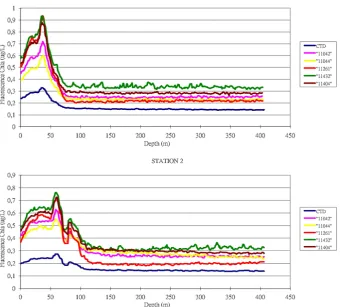
Figure 2.Example of fluorescence profiles provided by different CTD-FLUO-SRDLs and the reference fluorometer (in blue) obtained at
two different stations. These profiles exhibit the existence of a fluorescence offset differing between CTD-FLUO-SRDLs. Fluorometers were
providing consistent data between each other, but differed in the absolute amount of fluorescence produced.
2.2.3 Post deployment issues and correction processes Chlasaturated values
According to chl a measurements available for the study area ft02, ft03, ft04 CTD-Fluoro SRDL Tags the Cyclops 7 fluo-rometer gain was set to monitor chl a concentration ranging between 0 and 2.5µg L−1. In situation of high in situ chl a concentration, some raw profiles exhibited saturated values. Therefore, these profiles were flagged accordingly and re-tained as saturated one in the data base. For the ft06 Tags the gain of the Cyclops 7 fluorometer was set for a dynam-ical range of 0 to 4µg L−1and saturated chl a profiles were exceptionally encountered and flagged accordingly. Unsat-urated profiles were flagged as “1” while satUnsat-urated profiles were flagged as “2”.
Offset correction
Initially each in situ profiles was corrected according to the mean offset calculated for each tag from the at-sea test con-ducted prior to deployments which exhibited very little vari-ability for a given fluorometer between cast (see result part).
which were flagged as “3” and these flag 3 profiles are not integrated in the current data base.
Quenching correction
In both, laboratory and field studies, a daily rhythm of in vivo fluorescence that is not correlated with diel changes in the concentration of chl a have been reported in a number of studies. During periods of high irradiance, fluorescence tends to be lower than the value at night (Kiefer, 1973; Lof-tus and Seliger, 1975; Falkowski and Kolber, 1995; Dan-donneau and Neveux, 1997; Behrenfeld and Kolber, 1999; Kinkade et al., 1999). The photo-inhibition of phytoplankton by an excess of light, result in a decrease of the fluorescence quantum yield (i.e., the ratio of photons emitted as fluores-cence to those absorbed by photosynthetic pigments). This is often ascribed to a set of processes generally termed non-photochemical fluorescence quenching (NPQ; Falkowski and Kolber, 1995; Krause and Jahns, 2004). Quenching is com-monly observed during daytime with a maximum intensity at midday (Kiefer, 1973; Dandonneau and Neveux, 1997) and it is referred as daytime fluorescence quenching. Quenching poses a problem and, therefore, need to be accounted for. We applied the new method of quenching correction developed, tested and successfully applied to fluorescence data collected by elephant seals (Xing et al., 2012). In short, for mixed type waters, the maximum fluorescence values within the mixed layer is extended to the surface (i.e., all upper points are re-placed by this maximum value). However, for stratified wa-ters, which usually have a thin mixed layer, obviously, the quenching effect will pass through the mixed layer into the stratified layer. In the stratified layer, we were unable to per-form such correction and only night time fluorescence pro-files were used. However, the stratified layer situations were only encountered for 16 % of the fluorescence profiles sam-pled, and nearly half of them were obtained at night. In this process, we assume the maximum value in the mixed layer as the non-quenching value and all above points are corrected to the same value (see Xing et al., 2012). After implementing such corrections, no differences could be detected between day time fluorescence corrected profiles and the proximate night profiles (just before or after the day profiles).
2.2.4 Estimation of the tag specific chlacorrection coefficient: a Bayesian approach
Using a Bayesian adjustment framework and by combin-ing each at-sea test, the information available for each pro-file and the HPLC values available, a chl a calibration co-efficient was calculated for each CTD-Fluoro SRDL tag. A Bayesian framework is especially suited as it guarantees that between-casts variability is taken into account in estimat-ing these inter-fluorometer coefficients. An attractive feature of this framework is the relative ease with which different datasets are combined in a single analysis, allowing
infor-mation transfer between disparate sources. Another advan-tage stems from the easy computation of confidence inter-vals for parameters of interest and prediction errors. Models were fitted with WinBUGS (Spiegelhalter et al., 2003) called from R (R Development Core Team, 2009) with the package
R2WinBUGS (Sturtz et al., 2005). Weakly informative and
robust priors were favoured. We used uniform priors (Gel-man, 2006) for standard deviation parameters. Because all slopes were expected to be positive, we used Student-t priors with mean 0, scale 10 and 7 df on a log scale (Gelman et al., 2008). Batches of tag-specific coefficient were assumed to follow a bivariate Gaussian distribution with covariance ma-trixP. We used the prior described in Tokuda et al. (2011)
for the covariance matrixP.
We built a model to predict HPLC [chl a] from either in situ fluorescence (Fluo) measured by instrumented SES or from MODIS chl. Specifically we first used long-term data at the Boussole site to estimate the relationship between HPLC [chl a] and measurement from the reference fluorometer: HPLC [chl a]=δ·Fluo[reference]+ε1 (2) whereε1 is a Gaussian residual error term.
Secondly, we used data from the intercalibration experi-ment to estimate the relationship between a specific tag j and the reference fluorometer:
Fluo[reference]=αj·(Fluo j−Offset j)+ε2 (3) whereε2 is a Gaussian residual error term. When measure-ments from the reference fluorometer were unavailable, but measurements from the different tags at a specific location were available, we rewrote Eq. (3) as:
Fluo[reference]−(αj·(Fluo j−Offset j)+ε2)=0 (4) and put a weakly informative prior (Half-Student-t with mean 0, scale 5 and 4 df, Gelman et al., 2008) on the value of Fluo[reference]. We then used the WinBUGS “zero-trick”
(Spiegelhalter et al., 2003) to incorporate these data into the model. Note that the error termε2 is the same for Eqs. (3) and (4).
22 C. Guinet et al.: Calibration procedures and first dataset of Southern Ocean chlorophyllaprofiles
Table 1.Details of the 23 CTD-fluo tags deployments. Deployment date, Sampling period, number of fluoro-profiles obtained, and correction
coefficient applied to each tag.
Deployment number
CTD-Fluo SRDL number
Deployment date
End trans-mission
number of fluorescence profiles collected
number of fluorescence profiles usable
Daylight hours profile
night hours profile
nb of saturated profile
nb of quenching corrected profile
nb prof flag 1 offset profile
nb of prof flag 2 Offset profile
Mean offset (predeploy-ment sea test)
FT01 10863 12/22/2007 6/5/2008 241 241 166 75 32 76 212 29 – FT02 10946 1/20/2009 12/20/2009 331 331 187 144 1 145 248 83 1.28 FT02 11034 1/20/2009 3/12/2009 73 73 45 28 0 15 40 33 0.36 FT02 11035 1/28/2009 9/21/2009 404 404 202 202 0 148 292 112 0.44 FT02 11039 1/25/2009 7/13/2009 289 289 169 120 51 122 215 74 0.72 FT02 11040 1/20/2009 2/16/2009 41 41 26 15 1 13 30 11 0.43 FT02 11042 12/24/2008 6/1/2009 236 229 118 111 33 113 146 83 0.71 FT02 11044 1/10/2009 6/19/2009 267 267 139 128 92 66 238 29 0.51 FT03 11038 10/17/2009 12/31/2009 141 130 82 48 63 50 71 59 0.20 FT03 11259 10/19/2009 1/4/2010 134 125 72 53 35 50 85 40 0.17 FT03 11260 10/20/2009 1/9/2010 156 155 101 54 42 82 122 33 0.23 FT03 11262 10/23/2009 1/18/2010 169 169 114 55 45 100 144 25 0.28 FT03 11263 10/21/2009 1/9/2010 157 156 114 42 12 91 116 40 0.16 FT04 11042 3/8/2010 5/25/2010 97 51 0 51 0 0 38 13 0.24 FT04 11044 2/20/2010 8/19/2010 314 128 0 128 2 0 95 33 0.23 FT04 11261 2/15/2010 2/27/2010 13 6 0 6 1 0 4 2 0.21 FT04 11404 2/20/2010 9/25/2010 418 125 1 124 1 0 82 43 0.28 FT04 11432 3/12/2010 9/15/2010 309 112 0 112 0 0 87 25 0.33 FT06 10946 11/4/2010 1/19/2011 150 101 61 40 7 44 101 0
FT06 11035 11/4/2010 1/9/2011 120 102 84 18 35 53 102 0 0.30 FT06 11038 11/2/2010 1/25/2011 162 88 66 22 70 48 88 0
FT06 11262 10/22/2010 12/30/2010 136 6 3 3 0 2 6 0 0.24 FT06 11263 9/9/2010 11/24/2010 140 59 26 33 1 26 59 0 0.16
Total 4498 3388 1776 1612 524 1244 2621 767
Combining Eqs. (2) and (3) yields: HPLC [chl a]=δ·Fluo[reference]=δ·αj
·(Fluo j−Offset j) (6) whereδ·αj is a tag specific calibration coefficient allowing to predict HPLC [chl a] from in situ fluorescence. Combining Eqs. (5) and (6) further yields:
HPLC [chl a]=δ·αj·βj MODIS (7) which allows us to predict for each tag the likely value of HPLC [chl a] from MODIS measurement.
3 Results
3.1 At-sea trials prior to deployment
The at-sea testing previous to deployment revealed two types of issues which were tag’s fluorometer dependant: (1) a flu-orescence offset was, therefore, an instrument-specific clean water background, equivalent to the lowest values observed in the deepest part of the fluorescence profiles was subtracted from the raw fluorescence values; (2) for offset-corrected flu-orescence profiles, differences between tags in the absolute amount of fluorescence were detected.
The variability of the fluorescence offset for a given tag was one order of magnitude smaller than the offset diff er-ences between tags (Table 1). The mean fluorescent off -set for the tested tags during the BOUSSOLE cruise was
0.24±0.05µg L−1(range 0.16–0.33, n=14). For a given tag, the standard deviation of inter-cast fluorescent offset ranged from (0.0007 to 0.0620, mean=0.0148µg L−1).
3.1.1 Tag’s fluorometer intercalibration
The multiple cast performed during the at-sea test prior to ft03, ft04 and ft06 deployments allowed assessing the intra tag-fluorometer variability. This variability ranged from to a minimum of 0.03 % to a maximum of 5.61 % with a mean of 2.08±1.84 %. However, the difference between fluorometers was one order of magnitude larger than the within fluorom-eter variability and one fluoromenter provided fluorescence values which were on average 2.61 time higher than the min-imal values. The mean inter-fluorometer variation in fluores-cence values was 69 % (range 0.005 to 261 %).
On averageαj indicated that the tested fluorometers
pro-vided [chl a] 4 times greater (i.e., 0.24−1) than the reference fluorometer.
3.1.2 Reference fluorometer-HPLC relationship
C. Guinet et al.: Calibration procedures and first dataset of Southern Ocean chlorophyllaprofiles 23
which were on average 1.64 time greater than chl a concen-tration provided by concomitant HPLC measurements.
3.2 Post deployment data
From December 2007 to July 2010, a total of 27 SES, were fitted tags, of which 23 provided usable fluorescence data (Table 1). The 23 SES tracks provided a broad geographic and seasonal coverage ranging from Antarctic to subtropical waters, but with most individuals concentrating east of Ker-guelen Island within the KerKer-guelen plume (Fig. 4). A total of 4662 fluorescence profiles were transmitted, but 1274 of them either incomplete, with constant values or presenting obvious anomalies were discarded (i.e., 27 %). Among the remaining 3388 profiles 1776 were collected during the day and 1612 at night and year round (Fig. 5). The summary of the different profiles and flagging situation are provided in Table 1. This dataset (doi:10.7491/MEMO.1) is freely avail-able at http://www.cebc.cnrs.fr/ecomm/Fr ecomm/ecomm memoOCfd.html.
524 profiles exhibited saturated fluorescence values (i.e., 18 %) and were excluded for the comparison with the corre-sponding weekly chl a MODIS data. However, due to heavy cloud cover only 884 surface values of CTD-fluo profiles (i.e., 30.9 %) could be matched with the weekly MODIS data, and 126 with the MODIS data collected on the same day (i.e., 4.4 %).
Among these 23 tags deployed on SES, 8 were recovered when SES came back onshore after at sea periods ranging be-tween 3 to 8 months. At recovery the optical face of Cyclops 7 was clean with no bio-fouling most likely because elephant seals are typically deep divers spending very short periods within the euphotic zone. Furthermore, they spent most time at low temperatures.
On the 3388 fluorescence profiles, 40 % exhibited day time fluorescence quenching (i.e., 70 % of daytime profiles – Ta-ble 1). Therefore these profiles were corrected according to the procedure proposed by Xing et al. (2012). The recovery of fluorescence from quenching is obvious when we compare day profiles with night profiles obtained for the same loca-tion at the same date (Fig. 6). Individual seal collected chl a transects along their track monitoring latitudinal/longitudinal changes for a given time period as well as seasonal change within a given area (Fig. 7).
As quenching could only be corrected in well mixed water and not in stratified ones, we were (1) unable to proceed to quenching correction of fluorescence profiles in 283 profiles (i.e., about 16 % of daytime profiles) and therefore unable to assess properly deep maximum fluorescence for these day-time fluorescence profiles. To address this question we only used the 1612 night time profiles. Among those 352 had a maximum value at surface, while 742 exhibited a maximum deeper than 30 m. However, the vast majority the maxima was not exceeding the surface values by more than 30 % (i.e., 1423 profiles). Only 148 night profiles (i.e., 9 % of the
to-Figure 3.Relationship between the chl a concentration provided by the reference fluorometer and the chl a concentration estimated from HPLC measurements. This relationship was estimated over 70 test profiles ranging between 30 to 200 m and performed between 2002 and 2009.
tal number of night profiles) had a deep maximum exceed-ing 30 % of the surface value (maximum: 180 %). The depth class distribution of the maxima values exceeding 30 % of the surface value are shown in Fig. 8 and exhibit a clear bimodal distribution with a 30–40 m and a 70–80 m modes.
No obvious spatial structuring in the distribution of these profiles could be identified through the range of the SES.
Deep offset and quenching corrected surface fluorescence values provided by intercalibrated tags according to the ref-erence fluorometer (ft03, ft04 and ft06) were related to the corresponding MODIS chl a value along SES tracks. This re-lationship was implemented within the Bayesian framework to correct tag fluorescence values for which no at-sea test was performed previous to the deployment. For the ft02 de-ployment the proportionality found between tags, all tested simultaneously at sea was used. Following the Bayesian pro-cedure previously described the correction coefficients (δ·αj,
mean value) applied to each tag were calculated and are given in Table 2.
The surface [chl a] values derivated from by offset and quenching corrected profiles were found to be related to the 8-day-9 km MODIS chl a values. On average MODIS val-ues were 3.04 times (βj, range: 1.90–8.74) lower than the
corresponding tag fluorometer, and we found that on aver-age, MODIS tended to underestimate HPLC related [chl a] by a mean 1.99 (δ·αj·βj, range: 1.04–3.21) factor compared
to the in situ estimates provided by the inter-calibrated flu-orescence tag (Table 2, Fig. 9). The variability of βj (i.e.,
24 C. Guinet et al.: Calibration procedures and first dataset of Southern Ocean chlorophyllaprofiles
Fig. 4
Figure 4.Location of the fluorescence profiles along the tracks of 24 SES successfully equipped with a CTD-FLUO-SRDL and collected within the scope of this study (December 2007–January 2011).
Fig. 5
Figure 5.Monthly distribution of the fluorescence profiles.
the fluorometers were identical, nevertheless some large dif-ferences could be observed between fluorometers with αj
ranging between 0.11 and 0.36 (mean: 0.24) and those dif-ferences in themselves require those fluorometers to be inter-corrected between each other. For the SO total absence of chl a was never detected by MODIS with the lowest value ob-served of 0.06µg L−1 in our case, while in situ fluorescence
measurements suggest that total absence (±0.025µg L−1, i.e.,
the detection limit of the Cyclops 7 fluorometer) of chl a can be observed.
4 Discussion and conclusion
The fluorescence profiles collected by the SES within the SO, provides 3-D information on otherwise poorly sampled area such as the Antarctic sea-ice zone, an area were the ocean satellites are blinded by sea-ice and/or cloud cover. SES pro-vided an unequalled dataset of fluorescence profiles associ-ated with temperature and salinity measurements (i.e., den-sity) for a broad sector of the Indian part of the SO and this dataset represents a significant contribution in to understand-ing of the seasonal variation of phytoplankton biomass.
C. Guinet et al.: Calibration procedures and first dataset of Southern Ocean chlorophyllaprofiles 25
Figure 6.Example of unquenched night fluorescence profiles (top) and quenched day ones (bottom) collected on the same location and same period by a CTD-FLUO-SRDL deployed on a male SES for-aging over the Kerguelen plateau.
the long-term relationship established over several years and encompassing numerous at-sea test exhibit a very good lin-ear relationship (Fig. 3). Therefore, we suggest using this global relationship to transform the inter-calibrated fluores-cence values provided by the fluorometers to an actual esti-mation of [chl a] value. In a last step when there are sufficient surface fluorescence measurements coinciding with MODIS one, MODIS data can be used as a common but weak rela-tive (not absolute) reference between fluorometers as many issues are affecting the quality of the relationship: low num-ber of corresponding values, a poor temporal and spatial cor-respondence when using 9 km weekly data.
Due to logistical constraints, all the inter-calibrations were performed form at-sea test conducted in the north-west Mediterranean Sea. This could result in some differences in the absolute amount of chl a estimated from fluores-cence data in the SO and this point should be investigated in greater details in future studies. This procedure, nevertheless, presents the major advantage of producing a dataset in which all fluorometers are inter-calibrated with each other. Further-more the long-term relationship established between the ref-erence fluorometer and HPLC in the north-west Mediter-ranean Sea is likely to be robust as it was established over
Fig. 7
Figure 7. Top: female SES equipped with a CTD-FLUO-SRDL and section to the track followed by a juvenile SES female between January–April 2009. This female left Kerguelen on 12 January and reached the Antarctic shelf on 6 February. This female left the Antarctic shelf on 14 March, the female then remained associated with the marginal ice zone and the Antarctic divergence. Bottom: interpolated quenching corrected fluorescence profiles provided by
this SES along its track. This tag exhibited a fluorescence offset of
0.2µg L−1of chl a and Antarctic values higher than 2µg L−1were
saturated. The abrupt change in chl a concentration (km 2400) coin-cides with sea-ice formation which took place in mid march. These data show both the latitudinal change in the phytoplankton concen-tration along a north south transect performed during the inward trip (i.e., 1600 km south of Kerguelen 500 m isobath) and the transition in phytoplankton concentration in Antarctic waters from summer to fall (from km 1600 to 2400).
a broad range of years and seasons encompassing different phytoplankton assemblages.
One important result of this study was to show that MODIS may underestimate surface [chl a] compared to in situ measurements provided by the inter-calibrated fluorom-eters (Fig. 9). In situ chl a concentration provided by the flu-orometer was correlated with the MODIS, but data points were highly dispersed. This is not surprising due to the low spatial and temporal resolution of the MODIS data used to in-vestigate this relationship while surface values collected by the tags were associated with a unique location within that 9×9 km sector and, therefore, small scale variation which can be measured by the fluorometer are likely to be overlooked by the 9×9 km MODIS and weekly data.
26 C. Guinet et al.: Calibration procedures and first dataset of Southern Ocean chlorophyllaprofiles
Fig. 8
Figure 8.Depth distribution of chl a maxima exceeding 30 % of the surface values.
HPLC measurement or from calibrated fluorometer (Mitchell and Hansen, 1991; Dierssen and Smith, 2000; Holm-Hansen et al., 2004; Garcia et al., 2005) with standard algo-rithms typically underestimating chl a by 2–3 times (Kahru and Mitchell, 2010) which is consistent with our study, and up to 5 times (Dierssen, 2010). These errors are typically transferred to the estimates of primary production and car-bon fluxes.
Therefore, we are confident that the current MODIS data underestimate by a large extent the in situ [chl a]. In our study the MODIS underestimation was found over the whole study area and, therefore, encompassed a broad range of phy-toplankton assemblage. But future studies should investigate in greater details if the relationships between chl a surface concentration estimated from in situ fluorescence measure-ments and MODIS do vary according to the biogeographic regions of the SO visited by the SES. Furthermore, the in situ chl a/MODIS relationship is characterised by an inter-cept which is different from 0. A recent study reveals that within the SO the current ocean colour algorithms signifi-cantly underestimate and overestimate chl a at high and low concentrations, respectively (Johnson et al., 2013).
Global estimates of ocean primary production are now based on satellite Ocean Colour data (Longuhurst et al., 1995; Antoine et al., 1996; Behrenfeld and Falkowski, 1997; Behrenfeld et al., 2005). Time series have been built, from which climate-relevant trends can be extracted (Antoine et al., 2005; Polovina et al., 2008; Martinez et al., 2009). In situ and satellite data are highly complementary. Whereas in situ data extend the satellite information into the ocean interior (unseen by the remote sensor) and provide indispensable sea truth data, satellite provides the synoptic coverage.
We also found that when taking into account the quench-ing effect, deep maxima chl a concentration exceeding 30 % of the surface value were found only in 9 % of the night
pro-Fig. 9
Figure 9. Relationship between the offset, quenching corrected HPLC inter-calibrated fluorometers with the corresponding 9 km weekly MODIS data. Both regressions with (in red) and without (in black) intercept are presented.
file. According to this result the decoupling of surface and deep phytoplankton biomass observed for only 9 % of the profiles is unlikely to be a major issue when estimating pri-mary production from surface data. However, the real issue is the quenching effect observed during daylight hours and requiring to be properly dealt with (Xing et al., 2012).
Models can only provide useful answers if there are suffi -cient data to constrain the underlying processes and validate the model output. New approaches to assimilate biological and chemical data into these models are advancing rapidly (Brasseur et al., 2009). Notably, the progressive integration of biogeochemical variables in the next generation of opera-tional oceanography systems is one of the long-term objec-tives of the GODAE OceanView international programme. Nevertheless, and in view of refining these models for im-proving their representativeness and predictive capabilities, the datasets currently available remain too scarce. There is an obvious and imperative need to reinforce biological and bio-geochemical data acquisition and to organise databases and SES equipped with CTD-Fluo SRDL tags are contributing efficiently to this need.
In situ acquisition of fluorescence data by SES represents a significant contribution to the observation of biogeochemi-cal and ecosystem variables within this undersampled Ocean. These new data implemented in tight synergy with two other essential bricks of an integrated ocean observation system: modelling and satellite observation should represent a signif-icant contribution towards the resolution of important scien-tific questions relative to the overall phytoplankton biomass and primary production and ultimately changes in carbon fluxes within the SO in relation to climate variability and longer term changes.
Supplementary material related to this article is
Table 2.Correction coefficient calculated for each fluorometer tag (see methods for details). The bold values refer to the correction coefficient applied to the corresponding fluorometer tag, to estimate [chl a].
Deployment CTD-Fluo SRDL αj βj δ·αj δ·αj·βj number number Mean Lower Upper Mean Lower Upper Mean Lower Upper Mean Lower Upper
FT01 10863 0.26 0.13 0.46 2.96 2.20 3.77 0.65 0.32 1.16 1.91 0.92 3.52 FT02 10946 0.24 0.12 0.45 4.74 4.44 5.04 0.61 0.30 1.14 2.90 1.41 5.38 FT02 11034 0.33 0.18 0.50 2.08 1.65 2.51 0.83 0.47 1.26 1.73 0.93 2.72 FT02 11035 0.29 0.17 0.42 1.90 1.74 2.06 0.74 0.44 1.08 1.39 0.83 2.08 FT02 11039 0.14 0.09 0.20 8.74 7.77 9.75 0.36 0.22 0.51 3.12 1.88 4.49 FT02 11040 0.24 0.14 0.35 3.49 2.90 4.07 0.61 0.36 0.89 2.11 1.22 3.20 FT02 11042 0.19 0.12 0.27 3.50 3.32 3.67 0.48 0.30 0.68 1.67 1.05 2.36 FT02 11044 0.22 0.14 0.32 1.81 1.44 2.21 0.57 0.35 0.81 1.02 0.59 1.50 FT03 11038 0.11 0.10 0.12 3.58 2.74 4.46 0.28 0.25 0.31 1.00 0.75 1.28 FT03 11259 0.23 0.21 0.26 2.42 1.77 3.10 0.59 0.52 0.66 1.42 1.02 1.86 FT03 11260 0.22 0.19 0.24 2.07 1.69 2.44 0.54 0.48 0.61 1.13 0.89 1.36 FT03 11262 0.22 0.19 0.25 3.79 3.38 4.18 0.56 0.49 0.63 2.10 1.77 2.45 FT03 11263 0.27 0.23 0.30 2.29 1.90 2.71 0.67 0.59 0.76 1.54 1.23 1.89 FT04 11042 0.30 0.22 0.38 3.42 2.99 3.87 0.76 0.57 0.96 2.61 1.89 3.41 FT04 11044 0.35 0.26 0.45 2.61 2.24 3.01 0.89 0.66 1.15 2.33 1.65 3.09 FT04 11261 0.24 0.18 0.30 2.39 1.56 3.28 0.61 0.46 0.75 1.45 0.88 2.13 FT04 11404 0.25 0.19 0.31 5.07 4.51 5.64 0.63 0.48 0.80 3.21 2.37 4.14 FT04 11432 0.24 0.18 0.31 2.83 2.51 3.18 0.62 0.46 0.78 1.75 1.28 2.25 FT06 10946 0.24 0.12 0.45 4.06 3.68 4.45 0.61 0.31 1.13 2.49 1.24 4.59 FT06 11035 0.36 0.32 0.39 3.11 2.48 3.74 0.90 0.81 0.99 2.80 2.19 3.42 FT06 11038 0.25 0.12 0.46 4.24 2.99 5.60 0.62 0.30 1.16 2.63 1.20 5.23 FT06 11262 0.36 0.32 0.39 2.72 1.58 3.91 0.90 0.82 0.99 2.45 1.44 3.55 FT06 11263 0.21 0.19 0.23 1.95 1.44 2.45 0.53 0.48 0.58 1.04 0.76 1.32
Mean 0.24 0.20 0.29 3.04 2.53 3.57 0.61 0.51 0.73 1.99 1.44 2.33
Acknowledgements. This work was supported by CNES-TOSCA (Southern Elephant Seal as oceanographer Fluorescence measurements), The MEMO observatory as part of the SOERE CTD-02, the ANR VMC IPSOS-SEAL (2008–2011) and the Total Foundation. We are indebted to IPEV (Institut Polaire Franc¸ais), for financial and logistical support of Antarctic research program 109 (Seabirds and Marine Mammal Ecology lead by H. Weimerskirch). Special to the BOUSSOLE cruise and team for their help in proceeding at-sea tests and to F. Roquet who proceeded to the
correction/validation of the temperature/salinity data. Finally, we
would like to thank all the colleagues and volunteers involved in the field work on southern elephant seals at Kerguelen Island, with the special acknowledgement of the invaluable field con-tribution of N. ElSkaby, G. Bessigneul, A. Chaigne and Q. Delorme.
Edited by: F. Schmitt
References
Antoine, D., Andr´e, J. M., and Morel, A.: Oceanic primary pro-duction 2. Estimation at global scale from satellite (coastal zone color scanner) chlorophyll, Global Biogeochem. Cy., 10, 57–69, 1996.
Antoine, D., Morel, A., Gordon, H. R., Banzon, V. F., and Evans R. H.: Bridging ocean color observations of the 1980s and 2000s in search of long-term trends, J. Geophys. Res., 110, C06009,
doi:10.1029/2004JC002620, 2005.
Antoine, D., D’Ortenzio, F., Hooker, S. B., B´ecu, G., Gentili, B., Tailliez, D., and Scott, A. J.: Assessment of uncertainty in the ocean reflectance determined by three satellite ocean
color sensors (MERIS, SeaWiFS, and MODIS-A) at an offshore
site in the Mediterranean Sea, J. Geophys. Res., 113, C07013,
doi:101029/102007JC004472, 2008.
Argos: User’s manual, CLS/Service Argos, Toulouse, 1996.
Arrigo, K. R., Worthen, D. L., Schnell, A., and Lizotte, M. P.: Pri-mary production in Southern Ocean waters, J. Geophys. Res., 103, 587–600, 1998.
Babin, M.: Phytoplankton fluorescence: theory, current litterature and in situ measurements, in: Real-time coastal observing sys-tems for marine ecosystem dynamics and harmful algal blooms, edited by: Babin, M., Roesler, C., and Cullen, J. J., 237–280, Un-esco, Paris, 2008.
Babin, M., Morel, A., and Gentili, B.: Remote sensing of sea sur-face sun-induced chlorophyll fluorescence: Consequences of nat-ural variations in the optical characteristics of phytoplankton and the quantum yield of chlorophyll a fluorescence, Int. J. Remote Sens., 17, 2417–2448, 1996.
Behrenfeld, M. J. and Falkowski, P. G.: Photosynthetic rates de-rived from satellite-based chlorophyll concentration, Limnol. Oceanogr., 42, 1–20, 1997.
Behrenfeld, M. J. and Kolber, Z. S.: Widespread iron limitation of phytoplankton in the south Pacific Ocean, Science, 283, 840– 843, 1999.
28 C. Guinet et al.: Calibration procedures and first dataset of Southern Ocean chlorophyllaprofiles
doi:10.1029/2004GB002299, 2005.
Behrenfeld, M. J., O’Malley, R. T., Siegel, D. A., McClain, C. R., Sarmiento, J. L., Feldman, G. C., Milligan, A. J., Falkowski, P. G., Letelier, R. M., and Boss, E. S.: Climate-driven trends in con-temporary ocean productivity, Nature, 444, 752–755, 2006. Biuw, M., Boehme, L., Guinet, C., Hindell, M., Costa, D.,
Char-rassin, J. B., Roquet, F., Bailleul, F., Meredith, M., Thorpe, S.,
Tremblay, Y., McDonald, B., Park, Y.-H., Rintoul, S., Bindoff,
N., Goebel, M., Crocker, D., Lovell, P., Nicholson, J., Monks, F., and Fedak, M.: Variations in behaviour and condition of a Southern Ocean top predator in relation to in-situ oceanographic conditions, P. Natl. Acad. Sci. USA, 104, 13705–13710, 2007. Boehme, L., Meredith, M. P., Thorpe, S. E., Biuw, M., and
Fedak, M.: The Antarctic Circumpolar Current frontal sys-tem in the South Atlantic: Monitoring using merged Argo and animal-borne sensor data, J. Geophys. Res., 113, C09012,
doi:10.1029/2007JC004647, 2008.
Boehme, L., Lovell, P., Biuw, M., Roquet, F., Nicholson, J., Thorpe, S. E., Meredith, M. P., and Fedak, M.: Technical Note: Animal-borne CTD-Satellite Relay Data Loggers for real-time
oceano-graphic data collection, Ocean Sci., 5, 685–695, doi:10.5194/
os-5-685-2009, 2009.
Brasseur, P., Gruber, N., Barciela, R., Brander, K., Doron, M., El Moussaoui, A., Hobday, A. J., Huret, M., Kremeur, A.-S., Lehodey, P., Matear, R., Moulin, C., Murtugudde, R., Senina, I., and Svendsen, E.: Integrating Biogeochemistry and Ecology Into Ocean Data Assimilation Systems, Oceanography, 22, 206–215, 2009.
Buesseler, K. O., Barber, R. T., Dickson, M. L., Hiscock, M. R.,
Moore, J. K., and Sambrotto, R. N.: The effect of marginal
ice-edge dynamics on production and export in the Southern Ocean along 170-W, Deep-Sea Res. Pt. II, 50, 579–603, 2003.
Caldeira, K., Hoffert, M. I., and Jain, A.: Simple ocean carbon cycle
models, in: The Carbon Cycle, edited by: Wigley, T. M. L. and Schimel, D. S., Cambridge University Press, Cambridge, United Kingdom, 199–211, 2000.
Charrassin, J. B., Hindell, M., Rintoul, S. R., Roquet, F., Sokolov, S., Biuw, M., Costa, D., Boehme, L., Lovell, P., Coleman, R., Timmermann, R., Meijers, A., Meredith, M., Park Y.-H., Bailleul, F., Goebel, M., Tremblay, Y., Bost, C.-A., McMahon, C. R., Field, I. C., Fedak, M. A., and Guinet, C.: Southern ocean frontal structure and sea-ice formation rates revealed by elephant seals, P. Natl. Acad. Sci. USA, 105, 11634–11639, 2008. Dandonneau, Y. and Neveux, J.: Diel variations of in-vivo
fluo-rescence in the eastern equatorial Pacific an unvarying pattern, Deep-Sea Res., 44, 1869–1880, 1997.
Dierssen, H. M.: Perspective on empirical approaches for ocean color remote sensing of chlorophyll in a changing climate, P. Natl. Acad. Sci. USA, 107, 17073–17078, 2010.
Dierssen, H. M. and Smith, R. C.: Bio-optical properties and remote sensing ocean color algorithms for Antarctic Peninsula waters, J. Geophys. Res., 105, 26301–26312, 2000.
Falkowski, P. G. and Kolber, Z.: Variations in chlorophyll fluores-cence yields in phytoplankton in the world oceans, Aust. J. Plant Physiol., 22, 341–355, 1995.
Fedak, M., Lovell, P., McConnell, B., and Hunter, C.: Overcoming the Constraints of Long Range Radio Telemetry from Animals: Getting More Useful Data from Smaller Packages, Integr. Comp.
Biol., 42, 3–10, doi:10.1093/icb/42.1.3, 2002.
Field, C. B., Behrenfeld, M. J., Randerson, J. T., and Falkowski, P. G.: Primary production of the biosphere: Integrating terrestrial and oceanic components, Science, 281, 237–240, 1998. Garcia, C. A. E., Garcia, V. M. T., and McClain, C. R.:
Evalua-tion of SeaWiFS chlorophyll algorithms in the Southwestern At-lantic and Southern Oceans, Remote Sens. Environ., 95, 125– 137, 2005.
Gelman, A.: Prior Distributions for Variance Parameters in Hier-archical Models (Comment on Article by Browne and Draper), Bayesian Analysis, 1, 515–534, 2006.
Gelman, A., Jakulin, A., Grazia Pittau, M., and Su, Y.-S.: A Weakly Informative Default Prior Distribution for Logistic and Other Re-gression Models, Ann. Appl. Stat., 2, 1360–1383, 2008. Hindell, M., Slip, D., and Burton, H.: The diving behaviour of adult
male and female southern elephant seals, Mirounga leonina (Pin-nipedia: Phocidae), Aust. J. Zool., 39, 595–619, 1991.
Holm-Hansen, O., Kahru, M., Hewes, C. D., Kawaguchi, S., Kameda, T., Sushin, V. A., Krasovski, I., Priddle, J., Korb, R., Hewitt, R. P., and Mitchell, B. G.: Temporal and spatial distri-bution of chlorophyll-a in surface waters of the Scotia Sea as determined by both shipboard measurements and from satellite data, Deep-Sea Res. Pt. II, 51, 1323–1331, 2004.
Johnson, R., Strutton, P. G., Wright, S., McMinn, A., and Meiners, K. M.: Three Improved Satellite Chlorophyll Algorithms for the Southern Ocean, J. Geophys. Res., submitted, 2013.
Kahru, M. and Mitchell, G. B.: Blending of ocean colour algorithms applied to the Southern Ocean, Remote Sens. Lett., 1, 119–124, 2010.
Kiefer, D. A.: Fluoresence properties of natural phytoplankton pop-ulations, Mar. Biol., 22, 263–269, 1973.
Kinkade, C. S., Marra, J., Dickey, T. D., Langdon, C., Sigurdson, D. E., and Weller, R.: Diel bio-optical variability observed from moored sensors in the Arabian Sea, Deep-Sea Res. Pt. II, 46, 1813–1831, 1999.
Krause, G. H. and Jahns, P.: Non-photochemical energy dissipation determined by chlorophyll fluorescence quenching: characteriza-tion and funccharacteriza-tion, in: Chlorophyll a Fluorescence: A Signature of Photosynthesis, edited by: Papageorgiou, G. C., and Govindjee, Springer, Dordorecht, The Netherlands, 463–495, 2004. Lo Monaco, C., Goyet, C., Metzl, N., Poisson, A., and Touratier, F.:
Distribution and inventory of anthropogenic CO2in the
South-ern Ocean: Comparison of three data-based methods, J. Geophys.
Res., 110, C09S02, doi:10.1029/2004JC002571, 2005.
Loftus, M. E. and Seliger, H.: Some limitations of the in vivo fluo-rescence technique, Chesapeake Sci., 16, 79–92, 1975.
Longhurst, A., Sathyendranath, S., Platt, T., and Caverhill, C.: An estimate of global primary production in the ocean from satellite radiometer data, J. Plankton Res., 17, 1245–1271, 1995. Lydersen, C., Nøst, O. A., Lovell, P., McConnell, B. J.,
Gam-melsrød, T., Hunter, C., Fedak, M. A., and Kovacs, K. M.: Salin-ity and temperature structure of a freezing Arctic fjord monitored by white whales (Delphinapterus leucas), Geophys. Res. Lett.,
29, 2119, doi:10.1029/2002GL015462, 2002.
Marrari, M., Hu, C., and Daly, K. L.: Validation of SeaWiFS chloro-phyll a concentrations in the Southern Ocean: A revisit, Remote Sens. Environ., 105, 367–375, 2006.
Mitchell, B. G. and Holm-Hansen, O.: Bio-optical properties of
Antarctic Peninsula waters: Differentiation from temperate ocean
models. Deep-Sea Res., 38, 1009–1028, 1991.
Nicholls, K. W., Boehme, L., Biuw, M., and Fedak, M. A.: Win-tertime ocean conditions over the southern Weddell Sea con-tinental shelf, Antarctica, Geophys. Res. Lett., 35, L21605,
doi:10.1029/2008GL035742, 2008.
Polovina, J. J., Howell, E. A., and Abecassis, M.: Ocean’s least pro-ductive waters are expanding, Geophys. Res. Lett., 35, L03618,
doi:10.1029/2007GL031745, 2008.
Qu´eguiner, B. and Brzezinski, M. A.: Biogenic silica production rates and particulate organic matter distribution in the Atlantic sector of the Southern Ocean during austral spring, Deep-Sea Res. Pt. II, 49, 1765–1786, 2002.
R Development Core Team: R: A Language and Environment for Statistical Computing, R Foundation for Statistical Computing, Vienna, Austria, ISBN 3-900051-07-0, 2002.
Ras, J., Claustre, H., and Uitz, J.: Spatial variability of phytoplank-ton pigment distributions in the Subtropical South Pacific Ocean: comparison between in situ and predicted data, Biogeosciences,
5, 353–369, doi:10.5194/bg-5-353-2008, 2008.
Reynolds, R. A., Darius, S, and Mitchell, B. G.: A chlorophyll-dependent semianalytical reflectance model derived from field
measurements of absorption and backscattering coefficient
within the Southern Ocean, J. Geophys. Res., 10, 7125–7138, 2001.
Roemmich, D., Riser, S., Davis, R., and Desaubies, Y.: Autonomous profiling floats: Workhorse for broad-scale ocean observations, Mar. Technol. Soc. J., 38, 31–39, 2004.
Roquet, F., Park, Y. H., Guinet, C., and Charrassin, J. B.: Obser-vations of the Fawn Trough Current over the Kerguelen Plateau from instrumented elephant seals, J. Marine Syst., 78, 377–393, 2009.
Roquet, F., Charrassin, J. B., Marchand, S., Boehme, L., Fedak, M., Reverdin, G., and Guinet, C.: Validation of hydrographic data ob-tained from animal-borne satellite-relay data loggers, J. Atmos. Ocean Technol., 28, 787–801, 2011.
Spiegelhalter, D., Best, T., Best, N., and Lunn, D.: Winbugs user manual version 1.4, 2003.
Sturtz, S., Ligges, U., and Gelman, A.: R2winbugs: a Package for Running WinBUGS from R, J. Stat. Softw., 12, 1–16, 2005. Tokuda, T., Goodrich, B., Van Mechelen, I., Gelman, A., and
Tuer-linckx, F.: Visualizing Distributions of Covariance Matrices, Technical report, University of Leuwen, Belgium and Columbia
University, USA, available at: http://www.stat.columbia.edu/
∼gelman/research/unpublished/Visualization.pdf, 2011.
Uitz, J., Claustre, H., Griffiths, B., Ras, J., Garcia, N., and Sandroni,
V.: A phytoplankton class-specific primary production model ap-plied to the Kerguelen Isalnds region (Southern Ocean), Deep-Sea Res. Pt. I, 56, 541–560, 2009.
Waite, A. M. and Nodder, S. D.: The effect of in situ iron addition
on the sinking rates and export flux of Southern Ocean diatoms, Deep-Sea Res. Pt. II, 48, 2635–2654, 2001.
Wunsch, C., Heimbach, P., Ponte, R., Fukumori, I., and the ECCO-Consortium members: The global general circulation of the oceans estimated by the ECCO-Consortium, Oceanography, 22, 89–103, 2009.
Xing, X., Claustre, H., Blain, S., D’Ortenzio, F., Antoine, D., Ras, J., and Guinet, C.: Quenching correction for in vivo chlorophyll fluorescence measured by instrumented elephant seals in the Ker-guelen region (Southern Ocean), Limnol. Oceanogr.-Meth., 10, 483–495, 2012.
Yentsch, C. S. and Menzel, D. W.: A method for the determination of phytoplankton chlorophyll and phaeophytin by fluorescence, Deep-Sea Res., 10, 221–231, 1963.