https://doi.org/10.5194/gmd-11-1181-2018 © Author(s) 2018. This work is distributed under the Creative Commons Attribution 3.0 License.
Error assessment of biogeochemical models by lower bound
methods (NOMMA-1.0)
Volkmar Sauerland1, Ulrike Löptien2,3, Claudine Leonhard1, Andreas Oschlies2, and Anand Srivastav1 1Department of Mathematics, Kiel University, Christian-Albrechts-Platz 4, 24118 Kiel, Germany
2GEOMAR Helmholtz Centre for Ocean Research Kiel, Düsternbrooker Weg 20, 24105 Kiel, Germany 3Institute of Geosciences, Kiel University, Ludewig-Meyn-Strasse 10, 24118 Kiel, Germany
Correspondence:Volkmar Sauerland ([email protected]) Received: 6 June 2017 – Discussion started: 20 June 2017
Revised: 30 January 2018 – Accepted: 17 February 2018 – Published: 29 March 2018
Abstract.Biogeochemical models, capturing the major feed-backs of the pelagic ecosystem of the world ocean, are today often embedded into Earth system models which are increas-ingly used for decision making regarding climate policies. These models contain poorly constrained parameters (e.g., maximum phytoplankton growth rate), which are typically adjusted until the model shows reasonable behavior. System-atic approaches determine these parameters by minimizing the misfit between the model and observational data. In most common model approaches, however, the underlying func-tions mimicking the biogeochemical processes are nonlinear and non-convex. Thus, systematic optimization algorithms are likely to get trapped in local minima and might lead to non-optimal results. To judge the quality of an obtained pa-rameter estimate, we propose determining a preferably large lower bound for the global optimum that is relatively easy to obtain and that will help to assess the quality of an opti-mum, generated by an optimization algorithm. Due to the un-avoidable noise component in all observations, such a lower bound is typically larger than zero. We suggest deriving such lower bounds based on typical properties of biogeochemical models (e.g., a limited number of extremes and a bounded time derivative). We illustrate the applicability of the method with two world examples. The first example uses real-world observations of the Baltic Sea in a box model setup. The second example considers a three-dimensional coupled ocean circulation model in combination with satellite chloro-phylla.
1 Introduction
Earth system models are widely used to assess the conse-quences of climate change and explore climate engineering options (e.g., Brovkin et al., 2009; Keller et al., 2014; Mengis et al., 2015; Cao and Caldeira, 2008, 2010, and many more to follow). In order to capture the development of climate rele-vant greenhouse gases such as CO2and N2O a pelagic bio-geochemical component, embedded into a numerical ocean model, is essential.
optimization techniques to estimate the optimal model pa-rameters. These techniques require an objective metric (e.g., Evans, 2003) that measures the model–data misfit and can be minimized automatically. Due to computational limita-tions, various studies estimate the model parameters at sin-gular stations and adopt these for the full model (e.g., Kane et al., 2011; Kaufman et al., 2017; Matear, 1995; Schartau and Oschlies, 2003). For this approach, it can be problem-atic to determine a single parameter set for several sites (e.g., Kidston et al., 2011). Thus, other studies use fast approxima-tions (Kennedy et al., 2006; Khatiwala, 2007) to be able to optimize certain parameters for full three-dimensional mod-els. A drawback is that the latter approaches are generally restricted to the estimation of few parameters only (e.g., Mat-tern et al., 2012; Kriest et al., 2017; Prieß et al., 2013a, b; Pi-wonski and Slawig, 2016; Rückelt et al., 2010). In addition, limited data availability (e.g., Lawson et al., 1996) and a de-ficient representation of certain processes in the underlying ocean circulation model (e.g., Dietze and Löptien, 2013) en-cumber the optimization process. In summary, the systematic optimization of a 3-D coupled biogeochemical ocean model remains a difficult task and requires the advancement in ex-isting methods (Schartau et al., 2017).
Biogeochemical processes are nonlinear, non-convex, and complexly entangled. Therefore, as stressed by several fore-going studies, associated model–data misfit measures com-prise an unknown number of local optima and the results of an optimization provide no proof whether an obtained pa-rameter set is globally optimal or not (e.g., Faugeras et al., 2003; Hurtt and Armstrong, 1996). Many parameter opti-mization studies invoke deterministic methods that use gra-dient information about the objective function (the model– data misfit measure) to iteratively approach a locally opti-mal set of parameters in an efficient way, starting from some initial guess. Most of these studies calculate gradient infor-mation by the adjoint method (introduced for biogeochem-ical models by Lawson et al., 1995, since it is efficient if there are more parameters than model states) and use the gra-dient to determine a direction and an efficient step size to change the parameters, often by applying a quasi-Newtonian method (e.g., Fennel et al., 2001; Friedrichs, 2001, 2002; Spitz et al., 1998; Tjiputra et al., 2007; Xiao and Friedrichs, 2014). Other attempts focus on stochastic search algorithms which rely on random decisions. Examples for stochastic search algorithms that have been applied to optimize pa-rameters of biogeochemical models are simulated anneal-ing (e.g., Hurtt and Armstrong, 1996, 1999; Matear, 1995; Kidston et al., 2011), genetic algorithms (e.g., Hemmings and Challenor, 2012; Kaufman et al., 2017; Schartau and Os-chlies, 2003), and estimation of distribution algorithms (Kri-est et al., 2017). Vallino (2000) compares the performance of a couple of optimization algorithms of both types, tun-ing the parameters of an ecosystem model against mesocosm data. Stochastic search algorithms require more model sim-ulations (computation time) than gradient-based methods to
converge but are less likely to get trapped in a “first avail-able” local optimum (see Vallino, 2000), which might possi-bly be far off the global optimum. On the other hand, several contributions which focus on gradient-based methods aim to increase confidence in the quality of an obtained parame-ter set by repeating the optimization procedure many times (20–600), while using various random starting points (e.g., Garcia-Gorriz et al., 2003; Hemmings et al., 2004; Schartau et al., 2001). This approach also increases the number of re-quired simulations considerably.
Still, it is crucial to find a global optimum to assess the quality of a certain model formulation. Lacking a proof on the global optimality of chosen parameters, it is difficult to determine whether a model–data misfit is mainly caused by the parameter choice or attributed to other sources of un-certainty, like those concerning model equations or obser-vational data (see, e.g., Faugeras et al., 2003; Spitz et al., 1998; Schartau et al., 2001). Facing this situation, we have a strong interest to estimate the deviation of a model–data mis-fit for a given parameter set relative to the unknown global optimum. As the minimal accomplishable model–data misfit (i.e., the global optimum) is unknown, a good (i.e., preferably large) and easy-to-obtain lower bound on that value would help to judge the quality of a minimum obtained by an au-tomated optimization algorithm. Provided that such a lower bound is close to the obtained model–data misfit, a contin-uation of the parameter optimization process would not be necessary. In the present study, we introduce an approach to determine such lower bounds. We suggest considering a sur-rogate formulation that is easier to solve and determining the global optimum based on this “relaxed” problem. Our ap-proach is based on certain properties of typical biogeochem-ical models which are likewise fulfilled by non-parametric functions. We propose searching for the best fit to the obser-vations among these functions – which is a much easier and faster optimization problem than minimizing the model–data misfit based on the full biogeochemical model. Optimizing these non-parametric functions provides the desired bounds on the lowest possible misfit of the actual model, since the properties we choose to constrain the generalized optimiza-tion problems are satisfied by each soluoptimiza-tion of the original problem.
exam-ine the relation between both values depending on sparse-ness of the observational data and noise level. We further consider two real-world applications. The first application is based on a box model and investigates a common nutrients– phytoplankton–zooplankton–detritus (NPZD) biogeochemi-cal model in combination with phytoplankton observations in the Baltic Sea. Our second example is based on global satellite observations of chlorophyllaand a coupled biogeo-chemical ocean general circulation model.
2 Methods
Comparing model output to observational data requires a cri-terion to measure the misfit between both data sets. To apply an automated optimization algorithm, such a measure needs to be reduced to a single real number. We provide commonly used measures in the following subsection. In Sect. 2.2, we introduce mathematical notation for the optimization prob-lem based on the given measure for the model–data misfit. Additionally, we provide a mathematical formulation for the (simplified) non-parametric approach. We then give specifi-cations of the non-parametric data-fit problem based on fre-quency limits on the parameterized models (Sect. 2.3 and 2.4), bounds on their derivatives (Sect. 2.5), and the combi-nation of both (Sect. 2.6). These non-parametric relaxations will be used to calculate lower misfit bounds as outlined above.
2.1 Model–data misfit
A quality assessment of biogeochemical models usu-ally compares available observational datao=(o1, . . ., oN)
with corresponding model output (model predictions) p= (p1, . . ., pN).
For the sake of simplicity, we will consider scalar data in the following, assuming that bothoandpare univariate. Ac-tually, comprehensive global ocean models and observational data sets both comprise multiple quantities of interest on spa-tial grids. The presented lower bound methods can be utilized for that multi-variate case by applying them chunk-wise, for each quantity, and summing up the obtained results, option-ally using weights for the single terms.
Objective judgment about the differences between obser-vational data and model output requires an associated mea-sureferrthat assigns a real number to the model–data misfit. Furthermore, such an objective model–data misfit measure ferr has the advantage that it allows applying mathematical optimization algorithms to parametric models, where oth-erwise only manual parameter tuning can be done until the model output shows reasonable behavior.
There are several possible measures for the model–data misfit that have been used to evaluate biogeochemical mod-els (see, e.g., Evans, 2003; Gregg et al., 2009; Stow et al., 2009). Common measures are the mean absolute error
(MAE),
fmae(p,o)= 1 N
N
X
i=1
|pi−oi|,
and the root mean square error (RMSE),
frmse(p,o)= v u u t 1 N
N
X
i=1
(pi−oi)2.
It is sufficient to consider the following expression (sum of squared errors),
N
X
i=1
(pi−oi)2,
instead of RMSE as this transformation does not change the ranking of considered model outputsp. We will exemplarily work with RMSE which is the most commonly used misfit measure for biogeochemical models. However, our approach and the corresponding algorithms are transferable to other misfit measures like MAE.
2.2 The optimization problem
As mentioned above, we consider scalar observationso= (o1, . . ., oN)taken at timest1< t2<· · ·< tN. Moreover, we
introduce a scalar parametric model functionϕ:S×R→R, where the setS⊆Rnis the domain of the free parameters of the model. For a given parameter vectors∈S, the model pre-dictionp(s)=(p(s)1, . . ., p(s)N)at timest1< t2<· · ·< tN
is given byp(s)i =ϕ(s;ti). So, in order to determine
opti-mal model parameters, we want to minimize the model–data misfit measure
minXN
i=1(ϕ(s;ti)−oi) 2,
subject to s∈S,
(1)
numberα∈R>0which is as large as possible while satisfy-ing
α≤ N
X
i=1
(ϕ(s;ti)−oi)2 for alls∈S. (2)
Now, ifαsatisfies Inequality (2) and it holds for some model parameterss∈Sthat the corresponding model–data misfit is close toα, thensis a good parameter set with respect to the observational data (as well asαis a good lower bound on the unknown optimal model–data misfit).
In order to find such a lower boundα, our approach is to replace the parametric optimization problem (1) using a for-mulation that can be solved more easily. Therefore, we spec-ify a number of properties of the original model that hold for all parameter sets s∈S and which we require the alterna-tive formulation to fulfill. The global optimal value of such a relaxed problem is a lower boundα on the best possible model–data misfit of the original model. If the relaxed prob-lem is convex, in contrast to the original optimization task, its global optimum can be calculated efficiently (see, e.g., Boyd and Vandenberghe, 2004). We also refer to the infor-mation box below. Mathematically, our relaxations are mod-ifications of the original optimization task (1) in the sense that the parametric model function ϕ is replaced by a non-parametric function8from a classFof all functions that sat-isfy the considered property. In particular,Fcontainsϕ(s; ·) for all sfrom the parameter domainS of the actual model. The associated non-parametric optimization problem on the “extended search space” reads
minXN
i=1(8(ti)−oi) 2,
subject to 8∈F.
(3)
The model–data misfit of a global optimum of the relaxed problem (3) satisfies Inequality (2), meaning that it is a lower bound on the model–data misfit for all allowed parameterss of the original problem (1). We refer to Sect. 3 for thoughts on how the lower bound is employed in applications to judge the quality of the optimization outcome. In short, the main idea of the lower bound method can be summarized as fol-lows:
– Pick some properties that the model comprises for all parameterss∈S.
– Solve the optimization problem detached from the parametric model. Precisely, we minimize the sum of squared errors over all functions8∈F that fulfill the selected properties.
– The procedure yields a lower bound for the original op-timization problem as the set of possible solutions is larger for the relaxed problem and contains the original model output.
In the following sections, we give examples of the properties of the model that we choose.
Terms and background information
Given a functionf :Rn→R and a subsetX of Rn, a general mathematical optimization problem is
(MP) minimizef (x), subject tox∈X.
An example is the parameter optimization problem (1). Convex optimization problem.If f is a convex func-tion andXis a convex set, then (MP) is a called a con-vex optimization problem (CP). All relaxed problem for-mulations considered below are CPs. An important prop-erty of a CP is that every local optimum off overX is already a global optimum (see, e.g., Boyd and Vanden-berghe, 2004).
Quadratic program.A special CP is a convex quadratic program (QP). A QP has a convex quadratic objective function f and its function domain X is described in terms of someklinear constraints, i.e.,
X= {x∈Rn|gi(x)≥0 fori∈ {1, . . ., k}},
wheregi,i=1, . . ., k, are linear functions. The surrogate
model formulations (4)–(7) are QPs. Tools to calculate global optima of arbitrary QPs exist, but for most of our surrogates we can apply tailored algorithms which are more efficient.
2.3 Bounds for monotonic models
We start with an example that is not directly related to bio-geochemical models but which serves as a basis for the ap-proaches in Sect. 2.4 and 2.6, respectively. The task here is to fit observations with a monotonically increasing data set. Measuring the model–data misfit by its sum squared error, the associated non-parametric optimization problem can, for example, be stated as a convex quadratic program as follows
minXN
i=1(pi−oi) 2,
subject to p∈RN,
pi≤pi+1 fori∈ {1, . . ., N−1}.
(4)
This yields a vector p∈RN with monotonically increas-ing entries, wherepi is the data point that corresponds to
timeti. These entries are selected such that the sum of the
squared deviations from the observations is minimized. Note that Eq. (4) corresponds to the general non-parametric opti-mization problem (3) ifF is the class of all monotonically increasing functions. If we want to work with monotoni-cally decreasing functions instead, we just need to replace “≤” with “≥” in the monotonicity constraints or we can ap-ply Eq. (4) to−oinstead ofoand negate the result.
tj tk
Time
Va
l
u
e
Data
Perio dicmo del
Piece-wisemonotonicfit
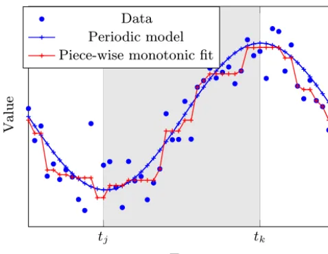
Figure 1.Synthetic data (blue dots) and corresponding output (blue crosses) of a periodic model function (blue curve). As the model fre-quencies are low, both the model function and its samples take only two local extremes. The segments before, after, and between the ex-tremes (timestj andtk) are monotonically decreasing/increasing. The respective monotonic fits to the data (drawn in red) are there-fore “better” than the model output.
1972) solves it with linear effort, i.e., in less thanc·N com-puter operations for some constant c and all N. Another possibility is to use a general optimization tool for con-vex quadratic programs like CPLEX or MATLAB quadprog. Clearly, solutions of Eq. (4) provide a lower bound on the optimal model–data misfit for every parametric model that is monotonically increasing.
2.4 Bounds for periodic models
When simulating periodic systems, the model might (inten-tionally or un-inten(inten-tionally) not resolve all frequencies that occur in the corresponding observational data. Models that resolve low frequencies with respect to data frequency (e.g., NPZD models that aim to capture the main characteristics of an annual cycle) take a correspondingly limited number of extreme values within a given time interval, e.g., a seasonal cycle. This situation is sketched in Fig. 1.
The fact that each segment between two subsequent ex-treme values is monotonically increasing/decreasing allows us to apply the methods introduced in Sect. 2.3. A corre-sponding seriesp1, . . ., pNof discrete samples has (at most)
the same number of local extremes as the model. For illus-tration, suppose that the series has exactly two extreme val-uespj andpkwithj < k∈ [N]as sketched in the example
in Fig. 1. These must be one minimum and one maximum. Assume that the time points j andk are known in advance and the minimum appears at position j. Then, an optimal data fit is a solution of a convex quadratic program similar
to Eq. (4)
minXN
i=1(pi−oi) 2,
subject to p∈RN,
pi≥pi+1 fori∈ {1, . . ., j−1}, pi≤pi+1 fori∈ {j, . . ., k−1}, pi≥pi+1 fori∈ {k, . . ., N−1},
pN≥p1
,
(5)
where the optional last constraint appears if the considered interval represents a full cycle of a periodic model. This yields a vectorp∈RNwith entries that decrease up to entry j, then start to increase, and fall after entryk. At the same time this vector minimizes the deviation from the observa-tional data. The negated solution of Eq. (5) applied to −o instead ofois an optimal data fit to observationsothat has a maximum at positionj and a minimum at positionk. Now, if the positionsjandkof the extremes are unknown, repeating the optimizations withoand−ofor everyj < k∈ [N], the best of all results is an optimal data fit subject to the property that there are (at most) two local extremes in the series. Sim-ilar to the case of two extremes, we can consider more than two, saym, extremes. Dealing with all possible combinations of the positions ofmextremes would imply a computational effort ofc1·Nm operations (c1 constant,N arbitrary), but using a tailored algorithm (Demetriou and Powell, 1991) we can calculate a best piece-wise monotonic fit in onlyc2·m·N2 computer operations.
2.5 Bounds for models with bounded derivatives
The change rates of biogeochemical processes like growth and decay have natural limits. In the presence of noise, ob-servational data are very likely to exhibit higher variations than a model that is devoted to comparatively slow interac-tions. In other words, noise (or unresolved periodic processes with high frequencies and high amplitudes) cannot be well approximated by models that mimic processes of lower vari-ation, i.e., models with small changes in a given time step. These processes are characterized by a small absolute tive. If we are able to postulate general bounds on the deriva-tives of a parametric model functionϕwith respect to time, we can try to utilize this property in order to calculate lower bounds on the optimal misfit ofϕ.
General bounds on the first time derivative (steepness) of ϕ are given as real numbers Dmin< Dmax such that Dmin≤ ∂ϕ∂t(s, t )≤Dmaxholds for all allowed parameter sets sand time pointst. Using the function spaceF= {8:R→
con-vex quadratic program minXN
i=1(pi−oi) 2,
subject to p∈RN,
pi+(ti+1−ti)Dmin≤pi+1 fori∈ [N−1], pi+(ti+1−ti)Dmax≥pi+1 fori∈ [N−1]. (6) A solution of this problem yields a lower model–data mis-fit bound for all parameter sets s such that ϕ(s,·) satisfies the steepness bounds,Dmin≤∂ϕ∂t(s, t )≤Dmax. Here, we ap-proximated the derivative 80(t )by finite differences which yieldsDmin≤8(tit+1)−8(ti)
i+1−ti ≤Dmax.
It is also possible to add linear constraints to the QP which consider bounds on higher-order derivatives of ϕ in terms of higher-order finite differences. For example, the property D2,min≤∂
2ϕ
∂t2(s, t )≤D2,max, s∈S, t∈ [t1, tN], can be ac-counted for with second-order differences by, for example, posing the (compactly written) constraints
D2,min≤
pi+2−2pi+1+pi (ti+2−ti)2
≤D2,max fori∈ [N−2]. The knowledge of tight bounds on derivatives of increasing order allows obtaining increasingly tight lower bounds on the model–data misfit. However, since bounds on higher-order derivatives are more difficult to derive in practice, we restrict our studies to steepness bounds.
2.6 Bounds for models with combined properties Clearly, we can combine model properties into a joint QP, e.g., if the model has two local extremes within a window of interest and bounded steepness. We can apply the combina-tion of Eqs. (5) and (6) and obtain the joint QP
minXN
i=1(pi−oi) 2,
subject to p∈RN,
pi≥pi+1≥pi+(ti+1−ti)Dmin fori∈ {1, . . ., j−1} ∪ {k, . . ., N−1}, pi≤pi+1≤pi+(ti+1−ti)Dmax
fori∈ {j, . . ., k−1},
pN≥p1≥pN+(T+t1−tN)Dmin
.
(7)
Here, again,j < kare the indices of the unique minimum and the unique maximum, respectively,Dmin<0 andDmax>0 are the universal lower and upper bounds on the model’s first derivative, andT is the optional period of the model.
Similar to the approach in Sect. 2.4, the optimal solution of Eq. (7) applied tooand−ofor allj < k∈ [N]will pro-vide the lower bound on the model–data misfit of the para-metric model. As an alternative to a QP solver, we can use an extension of the PAV algorithm that additionally considers
steepness bounds with monotonic regression called Lipschitz pool adjacent violators (LPAV; Yeganova and Wilbur, 2009) in order to solve Eq. (7).
3 Experiments 3.1 Method evaluation
We first aim to examine the extent to which the minimum model–data misfit of a parameterized model can deviate from the corresponding minimum misfit of a proposed non-parametric relaxation. Clearly, the difference between both misfits also depends on the characteristics of the observa-tional data, that is, noise level and data density. We there-fore derive statistics about that dependency using synthetic observations.
3.1.1 Test statistics
We generate the synthetic observations by adding white noise toN discrete samples8(ti)of a model function8:R−→ R, varying both the noise level and the number of samples. Our noise levels will be relative to the range
r:=max
i∈[N]8(ti) −min
i∈[N]8(ti)
of the model output. As a simple parametric test function we use a cubic polynomial 8(t )=ϕ(s, t )=
3 P
i=0
siti. We
sim-ulate 1-year time series of observational data by consider-ing the interval [0,365]and taking N equidistant samples, ti=Ni ·365, for a polynomial with fixed coefficients s∗ (a
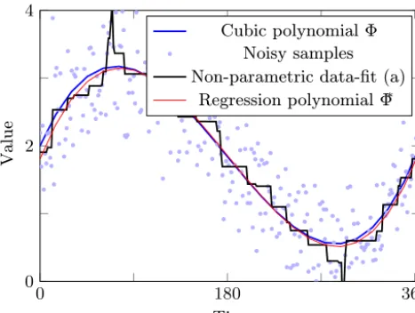
fixed parametrization), and N∈ {12,25,50,100,200,300}. We add zero-mean white noise N(0, σ ) to the time series values using one of six different noise levels with standard deviationsσ=σ∗·r,σ∗∈ {0.1,0.2,0.3,0.5,0.7,1.0}. Fig-ure 2 shows the exemplary cubic polynomial
8(t )=2+0.035·t−0.0003·t2+5.592·10−7·t3
andN=300 synthetic observationsoi obtained by adding
white noise with standard deviationσ =0.2·r to the cor-responding function values, i.e.,oi=8(ti)+N(0,0.2·r).
The figure further shows the minimum RMSE data fit by a function that has at most two local extremes as introduced in Sect. 2.4.
The related RMSE between the synthetic data and this piece-wise monotonic fit is 0.445. We know that this er-ror cannot be larger than the corresponding erer-ror between the fix polynomial 8 and the data since any cubic poly-nomial also takes at most two extremes. Indeed, the latter error is 0.501, which is the RMS of the white noise we added. By solving a convex optimization problem we can efficiently identify the coefficientss∗=(s0∗, s1∗, s2∗, s3∗)of a polynomial8∗=
3 P
i=0
0 180 360 0
2 4
Time
Va
l
u
e
Cubicp olynomialΦ
Noisysamples
Non-parametricdata-fit(a)
Regressionp olynomialΦ
∗
Figure 2.A cubic polynomial, synthetic observational data gener-ated by adding white noise to 300 equidistant samples of the poly-nomial, and a minimum RMSE data fit with regard to the property that no more than two extremes are taken.
cubic polynomials. Unsurprisingly, the re-optimized polyno-mial8∗differs only slightly from the original one and yields a RMSE of 0.497.
For our statistics about the proposed error assessment methods we are interested in the ratio
q:= frmse(p
rel,o) frmse(ppar,o)
between the lower error bound given by the optimal output of a non-parametric model relaxationpreland the correspond-ing data fit with the original parametric model ppar. In the above example this ratio is qa=00..445501 =0.888∼89 %. We repeat the calculation of a lower error bound and the cor-responding error ratio with two other relaxations assuming only a bounded model steepness (see Sect. 2.5) and a com-bination of both properties, bounded steepness and the exis-tence of at most two (local) extremes (see Sect. 2.6), respec-tively. The results are depicted in Fig. 3.
Here, for both relaxations we assume a maximum model steepness of 0.05 which is approximately 28 % more than the maximum steepness of the original polynomial in the interval
[0,365]. The resulting RMSEs of the property-based optimal data fits are 0.442 if only the steepness bound is assumed (data fit (b)) and 0.464 if both properties are assumed (data fit (c)). The corresponding error ratios are qb=0.883 and qc=0.927.
To derive robust statistics, we repeat the experiment 100 times using different zero-mean white noise with the same standard deviationσ. Now, we do the same for all 6×6 com-binations ofN andσ; i.e., we apply the three model relax-ations (a), (b), and (c) with regard to each of the 36 data prop-erty assumptions to 100 data sets of corresponding synthetic observations. The results are shown in Table 1.
0 180 360
0 2 4
Time
Va
lu
e
Noisy samples Data-¯t (b) Data-¯t (c)
Figure 3.The synthetic observational data of Fig. 2 and minimum RMSE data fits with regard to a steepness bound (data fit, (b)) as well as regarding both properties, bounded steepness and the exis-tence of at most two extremes (data fit, (c)).
The approach to calculate lower bounds on the model–data misfit by using property-based model relaxations stems from the intuition that the overall shape of the optimized paramet-ric model and that of the non-parametparamet-ric relaxation should be similar if the relaxation describes the main properties of the original model well. The amount of similarity is reflected by the ratios stated in Table 1. Values that are close to 100 % pro-vide epro-vidence that the parametric model is suitably shaped with regard to the corresponding general model property as-sumptions. Here, by construction of the synthetic data, we already know that the original polynomials are “correctly shaped”. Therefore, the numbers in the table actually reflect the tightness of the property-based relaxations and serve as circumstances under which the lower bound approach can succeed.
We observe that the data must be rather dense in order to reach good error ratios, especially with low levels of noise. This dependence is plausible because small numbers of ob-servations and low levels of noise cause small difference quotients oi+1−oi
ti+1−ti of the observations. However, the explicit steepness bounds, property (a), or implicit steepness bounds, property (b), which we use for the model relaxation must be considerably smaller than the difference quotients in order to provide a lower bound that is close to the model–data misfit of the optimized parametric model.
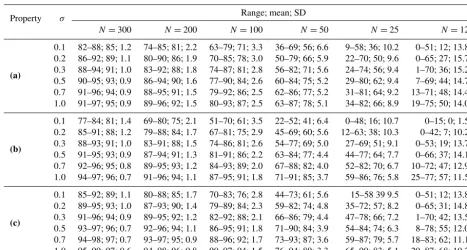
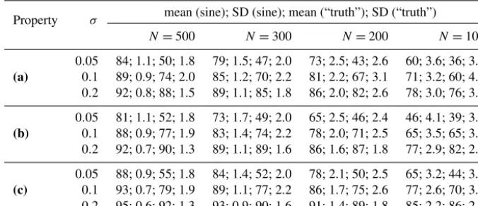
Table 1.Ratios (times 100) between the misfit of the parametric model (cubic polynomial) to synthetic observations (the model output plus white noise) and the misfit of the corresponding non-parametric regression model. We state the ratios for different noise levelsσ and numbers of samplesN. The values in each cell are the range of the ratios over 100 trials followed by their average and standard deviation. Non-parametric regression was done by(a)only assuming that at most two local extremes exist,(b)only assuming a steepness bound of 0.05, and(c)assuming both properties.
Property σ Range; mean; SD
N=300 N=200 N=100 N=50 N=25 N=12
(a)
0.1 82–88; 85; 1.2 74–85; 81; 2.2 63–79; 71; 3.3 36–69; 56; 6.6 9–58; 36; 10.2 0–51; 12; 13.8 0.2 86–92; 89; 1.1 80–90; 86; 1.9 70–85; 78; 3.0 50–79; 66; 5.9 22–70; 50; 9.6 0–65; 27; 15.7 0.3 88–94; 91; 1.0 83–92; 88; 1.8 74–87; 81; 2.8 56–82; 71; 5.6 24–74; 56; 9.4 1–70; 36; 15.2 0.5 90–95; 93; 0.9 86–94; 90; 1.6 77–90; 84; 2.6 60–84; 75; 5.2 29–80; 62; 9.4 7–69; 44; 14.7 0.7 91–96; 94; 0.9 88–95; 91; 1.5 79–92; 86; 2.5 62–86; 77; 5.2 31–81; 64; 9.2 13–71; 48; 14.4 1.0 91–97; 95; 0.9 89–96; 92; 1.5 80–93; 87; 2.5 63–87; 78; 5.1 34–82; 66; 8.9 19–75; 50; 14.0
(b)
0.1 77–84; 81; 1.4 69–80; 75; 2.1 51–70; 61; 3.5 22–52; 41; 6.4 0–48; 16; 10.7 0–15; 0; 1.5 0.2 85–91; 88; 1.2 79–88; 84; 1.7 67–81; 75; 2.9 45–69; 60; 5.6 12–63; 38; 10.3 0–42; 7; 10.2 0.3 88–93; 91; 1.0 83–91; 88; 1.5 74–86; 81; 2.6 54–77; 69; 5.0 27–69; 51; 9.1 0–53; 19; 13.7 0.5 91–95; 93; 0.9 87–94; 91; 1.3 81–91; 86; 2.2 63–84; 77; 4.4 44–77; 64; 7.7 0–66; 37; 14.1 0.7 92–96; 95; 0.8 89–95; 93; 1.2 84–93; 89; 2.0 67–88; 82; 4.0 52–82; 70; 6.7 10–72; 47; 12.9 1.0 94–97; 96; 0.7 91–96; 94; 1.1 87–95; 91; 1.8 71–91; 85; 3.7 59–86; 76; 5.8 25–77; 57; 11.5
(c)
0.1 85–92; 89; 1.1 80–88; 85; 1.7 70–83; 76; 2.8 44–73; 61; 5.6 15–58 39 9.5 0–51; 12; 13.8 0.2 89–95; 93; 1.0 87–93; 90; 1.4 79–89; 84; 2.3 59–82; 74; 4.8 35–72; 57; 8.2 0–65; 31; 14.8 0.3 91–96; 94; 0.9 89–95; 92; 1.2 82–92; 88; 2.1 66–86; 79; 4.4 47–78; 66; 7.2 1–70; 42; 13.5 0.5 93–97; 96; 0.7 92–96; 94; 1.1 86–95; 91; 1.8 71–90; 84; 3.9 54–84; 74; 6.3 8–78; 55; 12.0 0.7 94–98; 97; 0.7 93–97; 95; 0.9 88–96; 92; 1.7 73–93; 87; 3.6 59–87; 79; 5.7 18–83; 62; 11.1 1.0 95–99; 97; 0.6 94–98; 96; 0.8 90–97; 94; 1.5 76–94; 89; 3.3 65–90; 83; 5.1 29–87; 68; 10.2
level of 0.1 and property (a), the 85 % ratio is never reached in the worst case but only in the average case and only with N =300 observations.
3.1.2 A countercheck
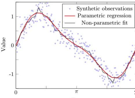
Having evidence that the lower bounds on the model–data misfit become tight with sufficiently dense observations, we want to countercheck if an optimized parametric model that slightly differs from the actual process behind the observa-tional data has a significantly worse model–data misfit in comparison with its non-parametric relaxation. This time, we generate 300 synthetic observations by disturbing the sum of two sine waves
8(t )=sin(t )+0.3·sin(2t )
and start with a noise level of 10 % relative to the range of the function values (σ=0.1·r). As the data might be mis-taken for noisy measurements of a single sine process at first glance, we use a general sine model to fit the observations. From the data, we estimate that both the frequency and the amplitude of the sine are at most 1.2. This implies a max-imum steepness of 1.44 and that the sine model takes no more than two extremes in [2, π], that is, according to the above notation, we use a type (c) model relaxation. Opti-mization yields a solution with a RMS model–data misfit
0 π 2π
-1 0 1
Time
Va
l
u
e
Syntheticobservations
Sineregression
Non-parametricfit
Figure 4.Synthetic data obtained by adding noise to the function 8(t )=sin(t )+0.3·sin(2t )and the optimized data fit by a clean sine wave (parametric model) and its property-based non-parametric re-laxation (steepness≤1.44, at most two extremes), respectively.
0 π 2π
-1 0 1
Time
Va
lu
e
Synthetic observations Parametric regression Non-parametric ¯t
Figure 5. Synthetic observations as in Fig. 4 but optimizing the “correct” parametric model and its property-based non-parametric relaxation (steepness≤2.21, at most four extremes).
With regard to the data density, the ratio qc=0.727 of both values is not completely convincing and, indeed, one can recognize a “failure in the model shape”. Now, we sup-pose the more precise process
ϕ(s, t )=s1+s2·sin(s3(t−s4))+s5·sin(s6(t−s7)), (8) resolving a second sine wave of higher frequency. We further suppose knowledge of the general bounds on both amplitudes
|s2| ≤1.2, |s5| ≤0.35 and on both frequencies |s3| ≤1.2,
|s6| ≤2.2. This implies that the steepness ofϕis bounded by 1.22+0.35·2.2=2.21. From the data, we can expect that the new model with optimized parameters also only takes two extremes in the interval[0,2π]. However, for the given bounds on the frequency and arbitrary parameters the model can take up to four extremes. Consequently, in addition to the steepness bound on the model, at most four extremes must be assumed to calculate the lower error bound on the best possible model–data misfit. Applying both assumptions, (i.e., using model property (c) from above) the exact opti-mum value of the model relaxation is∼0.217, while the opti-mized new parametric model comes down to∼0.193 provid-ing a clearly better model–data misfit ratioqc=0.891 than the pure sine model. The optimized parametric model curve is shown in Fig. 5.
We repeat the experiment with noise levels ofσ=5 % and σ =20 % for different numbers of equidistant observations N ∈ {500,300,200,100} and for all three property-based model-relaxation types (a), (b), and (c) used in Sect. 3.1.1. Again, we generate 100 different random sets of observations for each combination of σ andN. The results are depicted in Table 2.
The experiments help to identify conditions under which we may distinguish the “truth” from “distortions of the truth”. Sufficient conditions are given if the misfit ratio for
the true parametric model, say q1, is not too small, e.g., q1≥0.5, but the ratio for a moderate distortion of the true parametric model, sayq2, is essentially smaller. Depending on how closeq1 is to 1, we may say thatq2 is essentially smaller thanq1if either of the fractionsqq2
1 and 1−q1
1−q2 are con-vincingly less than 1, say q1
q2 ≤0.75 or 1−q2
1−q1 ≤0.5. We find that a rather low noise level is necessary to satisfy these con-ditions. As already observed in Sect. 3.1, high noise levelsσ provide rather tight lower bounds on the minimum-attainable model–data misfit of the “correct model type” if sufficient observations are available. Unfortunately, the corresponding lower bounds for a less accurate model become similarly close in this case. For properties (b) and (c) and fewer ob-servations, they can even exceed the lower misfit bounds for the “correct model” since we apply different uniform steep-ness bounds.
3.2 Application to real-world observations
We now consider two real-world examples with the aim of fitting chlorophyllaobservations.
3.2.1 Baltic Sea observations
Our first example considers observations from the Bornholm Basin in the Baltic Sea at 55.15◦N, 15.59◦E, dubbed station BY5. The data were provided by the Swedish Oceanographi-cal Data Center (SHARK) at the Swedish MeteorologiOceanographi-cal and Hydrological Institute (SMHI). BY5 was repeatedly sampled during 1962–2009. As there are relatively long periods with only sparse data, we merge all data into a climatological sea-sonal cycle. To derive phytoplankton (in nitrate units) from chlorophylla, we use a constant ratio of chlorophyll a to nitrate of 1.59 g Chla(mol N)−1. The considered seasonally adjusted time series comprises 175 observations of phyto-plankton.
Table 2.Ratios (times 100) between the misfit of the parametric model to synthetic observations (the model output plus white noise) and the misfit of the corresponding non-parametric regression model. The ratios are given for different noise levelsσ and numbers of samplesN. The four entries in each cell are the mean ratio of 100 trials, the standard deviation for the pure sine model, and the corresponding values for the “true” model that uses a sum of two sine waves. Non-parametric regression was done by(a)only assuming that at most two (four) local extremes exist,(b)only assuming a model specific steepness bound (see text), and(c)assuming both properties.
Property σ mean (sine); SD (sine); mean (“truth”); SD (“truth”)
N=500 N=300 N=200 N=100
(a)
0.05 84; 1.1; 50; 1.8 79; 1.5; 47; 2.0 73; 2.5; 43; 2.6 60; 3.6; 36; 3.3 0.1 89; 0.9; 74; 2.0 85; 1.2; 70; 2.2 81; 2.2; 67; 3.1 71; 3.2; 60; 4.2 0.2 92; 0.8; 88; 1.5 89; 1.1; 85; 1.8 86; 2.0; 82; 2.6 78; 3.0; 76; 3.9
(b)
0.05 81; 1.1; 52; 1.8 73; 1.7; 49; 2.0 65; 2.5; 46; 2.4 46; 4.1; 39; 3.3 0.1 88; 0.9; 77; 1.9 83; 1.4; 74; 2.2 78; 2.0; 71; 2.5 65; 3.5; 65; 3.6 0.2 92; 0.7; 90; 1.3 89; 1.1; 89; 1.6 86; 1.6; 87; 1.8 77; 2.9; 82; 2.6
(c)
0.05 88; 0.9; 55; 1.8 84; 1.4; 52; 2.0 78; 2.1; 50; 2.5 65; 3.2; 44; 3.1 0.1 93; 0.7; 79; 1.9 89; 1.1; 77; 2.2 86; 1.7; 75; 2.6 77; 2.6; 70; 3.5 0.2 95; 0.6; 92; 1.3 93; 0.9; 90; 1.6 91; 1.4; 89; 1.8 85; 2.2; 86; 2.6
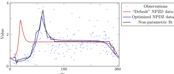
In a next step, we assess our result by examining the lower bounds. Following the procedure outlined at the end of Sect. 2.2, we need to identify properties of the NPZD model that are satisfied for every credible (allowed) parame-ter choice and lead to an easily solvable surrogate problem. Ideally, we could give mathematical proof of such properties. However, postulating a model property which is based on sound biological experience is justified, even if this property is not satisfied for all feasible combinations of the parameter values. In this context it is important to note that the rela-tively simple model structure of our NPZD model with fixed (non-temperature-dependent) rates does not suffice to de-scribe the seasonal cycle after the spring bloom (Fennel and Neumann, 2004, p. 35ff). Generally, model versions which fit the spring bloom satisfactory do not capture the observed chlorophyll increase in autumn. We thus assume only two extremes to determine a compatible lower bound. A practi-cal approach for more complex systems would be to itera-tively increase the number of extremes of the non-parametric model relaxation until the obtained lower bound hardly in-creases anymore (this approach would also require quite dense observational data). Using the algorithm of Yeganova and Wilbur (2009), we find that the best-attainable RMSE misfit between a time series with two extremes and our data isσa=0.557, a first lower error bound for the applied NPZD model. The corresponding error ratio between this bound and the error of the optimized model is qa=0.777. In or-der to tighten our lower error bound, we additionally postu-late a model steepness limit of 0.14, which we justify with the fact that the optimized model curve has two extremes, a plausible position of its maximum, and a maximal steep-ness of∼0.1. The associated best possible data fit, which we can calculate using the “piecewise monotonic regression” al-gorithm (Yeganova and Wilbur, 2009), in combination with
the LPAV algorithm (Demetriou and Powell, 1991) instead of the classical PAV algorithm (black curve in Fig. 6), has an RMSE of σc=0.66 which yields a quite high ratio of qc=0.σ717c =0.921. Thus, it is confirmed that the main por-tion of the model–data misfit of the optimized NPZD model is not caused by a sub-optimal choice of the parameter set but by other sources of uncertainty. For the sake of com-pleteness we calculate the best data fit with regard to a lim-ited model steepness of 0.14 solely (disregarding its number of extremes) using CPLEX to solve the corresponding for-mulation in terms of a quadratic program (6). In this case, the RMSE isσb=0.619 and the corresponding error ratio is qb=0.864.
0 180 360 0
2 4
Time
Va
l
u
e
Observations “Default”NPZDdata-fit OptimizedNPDZdata-fit
Non-parametricfit
Figure 6.Bornholm seasonally adjusted observation time series of phytoplankton, and data fits using the considered NPZD model using the parameters which were adjusted for global model configuration (red) and optimized parameters for the local model version (blue). The (black) reference plot is the minimum error data fit with regard to the properties that no more than two extremes are taken and the steepness is at most 0.14.
3.2.2 Global satellite observations
In a second example, we consider global observations of mar-itime chlorophylla. We use annual mean chlorophylla ob-servations in units of mg m−3, which were derived from Sea-WiFS satellite data from http://seadas.gsfc.nasa.gov (NASA Goddard Space Flight Center, 2011) using 8-day composites binned on a 1/12◦ spatial grid (4320×2160 boxes). Note that these annual averages might be seasonally biased in re-gions with sparse data. As we consider annual mean val-ues, we apply our method in space instead of time. We do not consider coastal areas, since these can not be well repre-sented in the coarse-resolution model and are also likely to contain a considerable degree of observational uncertainty. We thus mask out all grid boxes with chlorophylla concen-trations above 1 mg m−3. We compare the observed chloro-phyllaconcentrations to simulated values. The simulation is based on the CM2Mc configuration, described by Galbraith et al. (2010). Spinup procedure and boundary conditions fol-low Dietze et al. (2017) (see Table 1 their FMCD configura-tion). The resolution of the model comprises 120×80 boxes (3◦for longitudes and 2–3◦for latitudes) and is coarse com-pared to the spatial resolution of the observational data. The annual mean model simulations are interpolated onto the ob-servation grid in order to compute the corresponding RMSE for the model–data misfit. Figure 7 visualizes the observed chlorophyllaand the corresponding model simulations.
The observational data are quite rugged for larger regions of the ocean while the simulations are comparably smooth everywhere, due to the resolution of the model. Therefore, we can expect positive lower bounds on the model–data mis-fit.
The RMSE model–data misfit is 0.138 mg m−3. Deal-ing with two-dimensional data, our one-dimensional lower bound methods can be applied chunk-wise. Here, we traverse
each longitude of our spatial grid in chunks of 200 consecu-tive boxes (where the last chunk for each longitude consists of its≤200 remaining boxes). It provides with us a lower bound on the sum squared errors between observations and simulations with regard to each chunk, sayαi,k for thekth
ofni chunks of theith longitude,i∈ {1, . . .,4320}. A lower
bound on the (unweighted) RMSE model–data misfit is then given by
α=
v u u t
1 Nobs
4320 X
i=1
ni X
k=1 αi,k,
whereNobs is the total number of considered observation values. Note that the proposed method works equally well on weighted RMSEs. As a general model property for our bound approach we use a slightly higher maximum chloro-phyllavariation per distance than the maximum variation of our model simulation results (similar to the Baltic Sea exam-ple, we multiply the maximum simulated variation by 1.4 for each chunk). The result is a lower bound of 0.049 mg m−3 which is 35 % of the misfit we achieved with our model sim-ulations. Thus, the lower bound is in the same order of mag-nitude, but still considerably lower than the actual model– data misfit. One might conclude that there is room for model-improvement when it comes to chlorophylla. Still one needs to keep in mind that the model was presumably never op-timized to simulate chlorophyll a as good as possible and focused on many other factors as well.
Observed chlorophyll-a [mg/m3] Observedchlorophyll-a[mg m ]
-3
Simulated chlorophyll-a [mg/m3] Simulatedchlorophyll-a[mg m
-3]
−150−100 −50 0000 50 100 150
Longitude
−150−100 −50 0000 50 100 150
Longitude
−80
−60
−40
−20
0000
20 40 60 80
Latitude
−80
−60
−40
−20
0000
20 40 60 80
Latitude
XXXXXXXXXXXXXXXXXXXXXXXXXXXX
XXXXX
0.1 0.2 0.3 0.4 0.5 0.6 0.7 0.8 0.9 1.0
Figure 7.Observed and simulated annual mean chlorophyllamapped onto a 1/12◦spatial grid.(a)SeaWiFS level 3 mapped 8-day com-posites from http://seadas.gsfc.nasa.gov, 1998–2005 annual means of binned climatology.(b)Corresponding spatially interpolated model simulations.
4 Discussion
Our aim is to complement research on the calibration of bio-geochemical models by calculating lower bounds on their best-attainable model–data misfit. We utilize two general model properties for our purpose; a limited number of ex-tremes and a bounded model steepness. We also consider the combination of both properties. The reason to consider such non-parametric model properties is that they yield ef-ficiently solvable (relaxed) optimization problems whereas optimizing the original parametric model is computationally demanding.
4.1 Applicability
In our experiments (Sect. 3.1.1), the solitary assumption of a bounded model steepness leads to tight model relaxations (tight lower error bounds) if enough observational data are available and the steepness bound is chosen to be close to the maximum steepness of a calibrated model output. The task of deriving a maximal bound for the steepness of a re-spective model output can be difficult in practice and relies on (1) model equations and (2) observational data. A rig-orous mathematical model analysis, e.g., considering single model parameters like the maximum growth of phytoplank-ton, provides maximal limits which are valid for the entire parameter domain. However, relying on observation-based experience with the modeled processes, it might be justified to assume a smaller, empirical steepness bound, irrespective of that bound being valid for all permitted parameters. In Sect. 3.2.1, we assumed a steepness bound that is ∼40 % larger than the maximum steepness of the NPZD model with optimized parameters. In the future, we aim to target itera-tive procedures to derive tight universal (likely time variate)
model steepness bounds, e.g., using some kind of branch-and-bound approach.
Our second constraint, a limited number of extremes, is generally relatively easy to determine for common, rather smooth biogeochemical models. An applicable number of extremes can be determined if a regression with more ex-tremes only barely reduces the misfit any further. But here one should also keep the model structure in mind. Sim-ple models can be limited in reproducing specific shapes of the seasonal cycle. Based on the model structure, we as-sumed only two extremes for our NPZD real-world exam-ple in Sect. 3.2.1. Note, however, that assuming four ex-tremes yields better fits in this case: the RMSE decreases from 0.619 to 0.559 without bounding the steepness (from 0.66 to 0.62 with steepness bound). Note that the “low num-ber of extremes” condition indirectly implies a bounded (av-erage) model steepness, too. In our Baltic Sea experiments, the assumption about the number of extremes resulted in bet-ter bounds than the sole assumption of a bounded steepness. In our experiments with global ocean data, we observed op-posite results.
Unsurprisingly, the combination of tight steepness bounds with a limited number of extremes yields even better lower bounds on the minimum-attainable model–data misfit than both properties separately. Finally, all our model relaxations require a rather large number of observations (per chunk) in order to yield convincingly tight bounds (see Table 1). 4.2 Generalizations
corresponding tailor-made efficient algorithms. However, the suggested model properties also allow us to deduce optimiza-tion problems which are efficiently solvable if other misfit measures are used. For example, the sum absolute error can be dealt with in terms of linear programs (LPs) by including auxiliary variables and auxiliary linear constraints to express absolute values. Also, the efficient methods of Demetriou (1995) and Yeganova and Wilbur (2009) (we provide RMSE implementations in the Supplement) can be realized with other misfit measures than RMSE.
Concerning the number of local extremes, our proof-of-concept experiments are restricted to a maximum of two (four) extremes according to the properties of the respec-tive parametric models. However, solutions can even be cal-culated efficiently if the model output is assumed to take a large maximum number of extremes (Demetriou and Pow-ell, 1991; Demetriou, 1995). As mentioned above, a suitable approach to work with that property is to increase the max-imum assumed number of extremes until the corresponding lower bound on the minimum-attainable model–data misfit hardly increases anymore, indicating that further extremes contribute to fit noise rather than processes of interest. 4.3 Cautionary notes
Contrary to the fact that a small gap between the misfit of some property-based model relaxation and the misfit of the optimized original model proves that further parameter cali-bration is not required, a large gap between both misfits does not necessarily mean that the calibration of the chosen model is bad, nor does it mean that the model is an incorrect repre-sentation of the processes of interest. Our experiments indi-cate that a large gap only then tends to prove the inadequacy of a model (calibration) if enough observations are available. Otherwise, the chosen property-based relaxations might fit observations too well.
On the other hand, a small gap between the optimal misfit of a property-based non-parametric relaxation and the misfit of the original parametric model can even be reached with an inappropriate parametric model structure if there is too much noise in the data. The experiments in Sect. 3.1.2 are setup to estimate conditions that allow us to distinguish the “truth” from a “moderate distortion of the truth”. With regard to the experimental results in Table 2, a rather low noise level is necessary to satisfy these conditions.
5 Conclusions
We presented an approach for proving that a parametric model is well calibrated, i.e., that changes of its free param-eters can no longer lead to a much better model–data misfit. The intention is motivated by the fact that calibrating global biogeochemical ocean models is important but computation-ally expensive.
Generally, the aim is to determine an optimal parameter set such that a predefined metric of the model–data misfit is min-imal. To keep the number of required expensive model simu-lations as small as possible, we suggest calculating “tight” lower bounds on the lowest achievable model–data misfit. Our objective is to utilize properties of the original model that are satisfied for all permitted parameters and lead to eas-ily solvable optimization problems. Here, we focus on two such model properties to derive our lower bounds on the model–data misfit; a maximum time derivative and a max-imum number of extremes per time unit.
Indeed, our experiments show that the achieved bounds can come quite close to the optimized misfit of the original model if many observations are available. However, a prob-lem with global observational data (e.g., World Ocean Atlas data) is that it is often sparse in time. For example, if we examine annual cycles of periodic processes with monthly observations, our lower bound approach will only succeed if we overlay (seasonally adjust) measurement data of sev-eral years in order to reach the required data coverage. Long-term time series from observing platforms like BATS (Stein-berg et al., 2001) provide enough data on the temporal di-mension but are limited in space and are only available for certain sites. However, we can also apply our method with data that is dense in space. A suitable global application of our method to biogeochemical models is related with dense satellite observations of chlorophylla (Volpe et al., 2007; Dogliotti et al., 2009). Section 3.2.2 illustrates how our meth-ods can be applied in order to cope with such data.
Assuming the error between model output and observa-tions to be Gaussian distributed noise, an obtained lower bound on the RMSE is also a lower bound on the empirical standard derivationσ of the noise. We suggest the following rule-of-thumb procedure, which is illustrated for a real-world example in Sect. 3.2.1:
1. Optimize the model parameters with regard to the cor-responding model–data misfit.
2. Calculate lower error bounds on the model–data misfit by using appropriate assumptions about the model prop-erties.
Code availability. Implementations of the applied methods are available on GitHub (https://github.com/vsauerland/regression). A permanent version of the code described here is archived in the pub-lic Zenodo repository (Sauerland, 2017). We provide two packages of C++ sources:
– regressionCPXincludes QP formulations and requires the CPLEX solver.
– regression is a subset that does not require CPLEX, and only uses QP free and tailored regression algorithms: PAV (Barlow et al., 1972), LPAV (Demetriou and Powell, 1991), PMR (Yeganova and Wilbur, 2009), and a combination of LPAV and PMR, PMRS.
Appendix A: NPZD model parameters and equations We explicitly state the free parameters and equations of the NPZD box model that has been studied in Löptien and Dietze (2015) and is used for our real-world example in Sect. 3.2.1. The prognostic variables are nitrate (N), phytoplankton (P), zooplankton (Z), and detritus (D) and are scaled to units of mmol N m2. The temporal change of the prognostic variables depends on 10 free parameters outlined in Table A1 and is determined by the following equations
d
dtN= −µmax·gl·gN·P+mPN·P+mZN·Z+mDN·D, d
dtP=µmax·gl·gN·P−mPN·P−G(P)·Z−mPD·P, d
dtZ=G(P)·Z−mZN·Z−mZD·Z 2,
d
dtD=mZD·Z 2+m
PD·P−mDN·D.
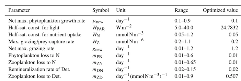
Table A1.Parameters of the considered NPZD model with their physical units, allowed ranges, and optimized values.
Parameter Symbol Unit Range Optimized value
Net max. phytoplankton growth rate µnew day−1 0.1–0.9 0.1
Half-sat. const. for light HPAR W m−2 5.0–40.0 24.7832
Half-sat. const. for nutrient uptake HN mmol N m−3 0.05–1.2 0.05
Max. grazing/prey-capture rate HZ mmol N m−6 0.2–1.1 0.2
Net max. grazing rate gnew day−1 0.01–1.2 1.2
Phytoplankton loss to N mPN day−1 0.01–0.6 0.01
Zooplankton loss to N mZN day−1 0.01–0.65 0.01
Remineralization rate of Det. mDN day−1 0.02–0.15 0.02
Zooplankton loss to Det. mZD day−1(mmol N m−3)−1 0.01–0.9 0.507
Phytoplankton loss to Det. mPD day−1 0.01–0.9 0.0191
Here, the hyperbolic MM equations gI=PARPAR+HPAR and
gN=N+NHN describe the limiting effect of light and nitrate concentration on the nitrate uptake of phytoplankton and
G(P)=gmax·P
2
P2+H Z
is a “Holling III” term. The maximum growth rate of phyto-planktonµmaxand the maximum grazing rate of zooplankton gmaxare obtained by substitutions
µnew:=µmax−mPN−mPD, gnew:=gmax−mZN,
Competing interests. The authors declare that they have no conflict of interest.
Acknowledgements. This work is a contribution to the the project “Reduced Complexity Models” (supported by the Helmholtz Asso-ciation of German Research Centres (HGF)), the DFG-supported project SFB754 and the DFG Cluster of Excellence “The Future Ocean”. The authors received very helpful comments from two anonymous reviewers. We are grateful to Heiner Dietze for technical assistance.
Edited by: Christoph Müller
Reviewed by: three anonymous referees
References
Anderson, T.: Plankton functional type modelling: running before we can walk?, J. Plankton Res., 27, 1073–1081, https://doi.org/10.1093/plankt/fbi076, 2005.
Aumont, O., Ethé, C., Tagliabue, A., Bopp, L., and Gehlen, M.: PISCES-v2: an ocean biogeochemical model for carbon and ecosystem studies, Geosci. Model Dev., 8, 2465–2513, https://doi.org/10.5194/gmd-8-2465-2015, 2015.
Barlow, R. E., Bartholomew, D. J., Bremner, J. M., and Brunk, H. D.: Statistical Inference under Order Restrictions, Theory and Application of Isotonic Regression, Wiley Series in Probabil-ity and Mathematical Statistics, John Wiley & Sons, London, https://doi.org/10.1111/j.1467-9574.1973.tb00228.x, 1972. Boyd, S. and Vandenberghe, L.: Convex optimization, Cambridge
University Press, 2004.
Brovkin, V., Petoukhov, V., Claussen, M., Bauer, E., Archer, D., and Jaeger, C.: Geoengineering climate by stratospheric sulfur injections: Earth system vulnerability to technological failure, Climatic Change, 92, 243–259, https://doi.org/10.1007/s10584-008-9490-1, 2009.
Cao, L. and Caldeira, K.: Atmospheric CO2 stabilization
and ocean acidification, Geophys. Res. Lett., 35, L19609, https://doi.org/10.1029/2008GL035072, 2008.
Cao, L. and Caldeira, K.: Atmospheric carbon dioxide removal: long-term consequences and commitment, Environ. Res. Lett., 5, 024011, https://doi.org/10.1088/1748-9326/5/2/024011, 2010. Demetriou, I. C.: Discrete piecewise monotonic approximation by a strictly convex distance function, Math. Comput., 64, 157–180, https://doi.org/10.2307/2153327, 1995.
Demetriou, I. C. and Powell, M. J. D.: Least squares smoothing of univariate data to achieve piecewise monotonicity, IMA J. Numer. Anal., 11, 411–432, https://doi.org/10.1093/imanum/11.3.411, 1991.
Dietze, H. and Löptien, U.: Revisiting nutrient trapping in global coupled biogeochemical ocean circulation models, Global Bio-geochem. Cy., 27, 265–284, https://doi.org/10.1002/gbc.20029, 2013.
Dietze, H., Getzlaff, J., and Löptien, U.: Simulating natural car-bon sequestration in the Southern Ocean: on uncertainties asso-ciated with eddy parameterizations and iron deposition, Biogeo-sciences, 14, 1561–1576, https://doi.org/10.5194/bg-14-1561-2017, 2017.
Dogliotti, A. I., Schloss, I. R., Almandoz, G. O., and Gagliardini, D. A.: Evaluation of SeaWiFS and MODIS chlorophyll-a products in the Argentinean Patagonian Conti-nental Shelf (38◦S-55◦S), Int. J. Remote Sens., 30, 251–273, https://doi.org/10.1080/01431160802311133, 2009.
Evans, G. T.: Defining misfit between biogeochemical models and data sets, J. Marine Syst., 40–41, 49–54, https://doi.org/10.1016/S0924-7963(03)00012-5, 2003. Faugeras, B., Lévi, M., Mémery, L., Verron, J., Blum, J.,
and Charpentier, I.: Can biogeochemical fluxes be recov-ered from nitrate and chlorophyll data? A case study assim-ilating data in the Northwestern Mediterranean Sea at the JGOFS-DYFAMED station, J. Marine Syst., 40–41, 99–125, https://doi.org/10.1016/S0924-7963(03)00015-0, 2003. Fennel, K., Losch, M., Schröter, J., and Wenzel, M.:
Test-ing a marine ecosystem model: sensitivity analysis and parameter optimization, J. Marine Syst., 28, 45–63, https://doi.org/10.1016/S0924-7963(00)00083-X, 2001. Fennel, W. and Neumann, T.: Introduction to the Modelling of
Ma-rine Ecosystems, Elsevier Science, ISBN 9780080534978, 2004. Friedrichs, M. A. M.: A data assimilative marine ecosys-tem model of the central equatorial Pacific: Numer-ical twin experiments, J. Mar. Res., 59, 859–894, https://doi.org/10.1357/00222400160497544, 2001.
Friedrichs, M. A. M.: Assimilation of JGOFS EqPac and Sea-WiFS data into a marine ecosystem model of the Central Equatorial Pacific Ocean, Deep-Sea Res. Pt. II, 49, 289–319, https://doi.org/10.1016/S0967-0645(01)00104-7, 2002. Friedrichs, M. A. M., Hood, R. R., and Wiggert, J. D.: Ecosystem
model complexity versus physical forcing: Quantification of their relative impact with assimilated Arabian Sea data, Deep-Sea Res. Pt. II, 53, 576–600, https://doi.org/10.1016/j.dsr2.2006.01.026, 2006.
Galbraith, E. D., Gnanadesikan, A., Dunne, J. P., and His-cock, M. R.: Regional impacts of iron-light colimitation in a global biogeochemical model, Biogeosciences, 7, 1043–1064, https://doi.org/10.5194/bg-7-1043-2010, 2010.
Garcia-Gorriz, E., Hoepffner, N., and Ouberdous, M.: Assim-ilation of SeaWiFS data in a coupled physical–biological model of the Adriatic Sea, J. Marine Syst., 40–41, 233–252, https://doi.org/10.1016/S0924-7963(03)00020-4, 2003. Gregg, W. W., Friedrichs, M. A., Robinson, A. R., Rose, K. A.,
Schlitzer, R., Thompson, K. R., and Doney, S. C.: Skill assess-ment in ocean biological data assimilation, J. Marine Syst., 76, 16–33, https://doi.org/10.1016/j.jmarsys.2008.05.006, 2009. Hemmings, J. C., Srokosz, M. A., Challenor, P., and Fasham,
M. J.: Split-domain calibration of an ecosystem model us-ing satellite ocean colour data, J. Marine Syst., 50, 141–179, https://doi.org/10.1016/j.jmarsys.2004.02.003, 2004.
Hemmings, J. C. P. and Challenor, P. G.: Addressing the impact of environmental uncertainty in plankton model calibration with a dedicated software system: the Marine Model Optimization Testbed (MarMOT 1.1 alpha), Geosci. Model Dev., 5, 471–498, https://doi.org/10.5194/gmd-5-471-2012, 2012.
Hurtt, G. C. and Armstrong, R. A.: A pelagic ecosystem model cal-ibrated with BATS and OWSI data, Deep-Sea Res. Pt. I, 46, 27– 61, https://doi.org/10.1016/S0967-0637(98)00055-7, 1999. Kane, A., Moulin, C., Thiria, S., Bopp, L., Berranda, M., Tagliabue,
A., Crépon, M., Aumont, O., and Badran, F.: Improving the pa-rameters of a global ocean biogeochemical model via variational assimilation of in situ data at five time series stations, J. Geophys. Res.-Oceans, 116, 1–14, https://doi.org/10.1029/2009JC006005, 2011.
Kaufman, D. E., Friedrichs, M. A. M., Hemmings, J. C. P., and Smith Jr., W. O.: Assimilating bio-optical glider data during a phytoplankton bloom in the southern Ross Sea, Biogeosciences, 15, 73–90, https://doi.org/10.5194/bg-15-73-2018, 2018. Keller, D. P., Feng, E. Y., and Oschlies, A.: Potential
cli-mate engineering effectiveness and side effects during a high carbon dioxide-emission scenario, Nat. Commun., 5, 3304, https://doi.org/10.1038/ncomms4304, 2014.
Kennedy, M. C., Anderson, C. W., Conti, S., and O’Hagan, A.: Case studies in Gaussian process modelling of com-puter codes, Reliab. Eng. Syst. Safe., 91, 1301–1309, https://doi.org/10.1016/j.ress.2005.11.028, 2006.
Khatiwala, S.: A computational framework for simulation of bio-geochemical tracers in the ocean, Global Biogeochem. Cy., 21, GB3001, https://doi.org/10.1029/2007GB002923, 2007. Kidston, M., Matear, R., and Baird, M. E.: Parameter
optimisa-tion of a marine ecosystem model at two contrasting staoptimisa-tions in the Sub-Antarctic Zone, Deep Sea Res. Pt II, 58, 2301–2315, https://doi.org/10.1016/j.dsr2.2011.05.018, 2011.
Kriest, I., Khatiwala, S., and Oschlies, A.: Towards an as-sessment of simple global marine biogeochemical mod-els of different complexity, Prog. Oceanogr., 86, 337–360, https://doi.org/10.1016/j.pocean.2010.05.002, 2010.
Kriest, I., Sauerland, V., Khatiwala, S., Srivastav, A., and Os-chlies, A.: Calibrating a global three-dimensional biogeochemi-cal ocean model (MOPS-1.0), Geosci. Model Dev., 10, 127–154, https://doi.org/10.5194/gmd-10-127-2017, 2017.
Lawson, L. M., Spitz, Y. H., Hofmann, E. E., and Long, R. B.: A data assimilation technique to a predator-prey model, B. Math. Biol., 57, 593–617, https://doi.org/10.1016/S0092-8240(05)80759-1, 1995.
Lawson, L. M., Hofmann, E. E., and Spitz, Y. H.: Time series sam-pling and data assimilation in a simple marine ecosystem model, Deep-Sea Res. Pt. II, 43, 625–651, https://doi.org/10.1016/0967-0645(95)00096-8, 1996.
Löptien, U.: Steady states and sensitivities of commonly used pelagic ecosystem model components, Ecol. Model., 222, 1376– 1386, https://doi.org/10.1016/j.ecolmodel.2011.02.005, 2011. Löptien, U. and Dietze, H.: Constraining parameters in marine
pelagic ecosystem models – is it actually feasible with typi-cal observations of standing stocks?, Ocean Sci., 11, 573–590, https://doi.org/10.5194/os-11-573-2015, 2015.
Löptien, U. and Dietze, H.: Effects of parameter indetermi-nacy in pelagic biogeochemical modules of Earth System Models on projections into a warming future: The scale of the problem, Global Biogeochem. Cy., 31, 1155–1172, https://doi.org/10.1002/2017GB005690, 2017.
Matear, R. J.: Parameter optimization and analysis of ecosystem models using simulated annealing: A case
study at station P, J. Marine Res., 53, 571–607, https://doi.org/10.1357/0022240953213098, 1995.
Mattern, J. P., Fennel, K., and Dowd, M.: Estimating time-dependent parameters for a biological ocean model us-ing an emulator approach, J. Marine Syst., 96–97, 32–47, https://doi.org/10.1016/j.jmarsys.2012.01.015, 2012.
Mengis, N., Keller, D. P., Eby, M., and Oschlies, A.: Uncer-tainty in the response of transpiration to CO2 and
implica-tions for climate change, Environ. Res. Lett., 10, 094001, https://doi.org/10.1088/1748-9326/10/9/094001, 2015.
NASA Goddard Space Flight Center: Sea-viewing
Wide Field-of-view Sensor (SeaWiFS)
Eu-photic Depth Data, NASA OB.DAAC,
Green-belt, MD, USA, https://doi.org/10.5067/ORBVIEW-2/SEAWIFS/L3M/ZLEE/2018 (last access: April 2011), 2018.
Oschlies, A. and Garcon, V.: An eddy permitting coupled physical-biological model of the North Atlantic. Part I: Sensitivity to ad-vection numerics and mixed layer physics, Global Biogeochem. Cy., 13, 135–160, https://doi.org/10.1029/98GB02811, 1999. Piwonski, J. and Slawig, T.: Metos3D: the Marine Ecosystem
Toolkit for Optimization and Simulation in 3-D – Part 1: Sim-ulation Package v0.3.2, Geosci. Model Dev., 9, 3729–3750, https://doi.org/10.5194/gmd-9-3729-2016, 2016.
Prieß, M., Koziel, S., and Slawig, T.: Marine ecosys-tem model calibration with real data using enhanced surrogate-based optimization, J. Comput. Sci., 4, 423–437, https://doi.org/10.1016/j.jocs.2013.04.001, 2013a.
Prieß, M., Piwonski, J., Koziel, S., Oschlies, A., and Slawig, T.: Ac-celerated parameter identification in a 3D marine biogeochemi-cal model using surrogate-based optimization, Ocean Model., 68, 22–36, https://doi.org/10.1016/j.ocemod.2013.04.003, 2013b. Rückelt, J., Sauerland, V., Slawig, T., Srivastav, A., Ward,
B., and Patvardhan, C.: Parameter Optimization and Uncer-tainty Analysis in a Model of Oceanic CO2 Uptake Using a Hybrid Algorithm and Algorithmic Differentiation, Non-linear Analysis B: Real World Applications, 11, 3993–4009, https://doi.org/10.1016/j.nonrwa.2010.03.006, 2010.
Sauerland, V.: Non-parametric optimization
meth-ods for model assessment (NOMMA-1.0),
https://doi.org/10.5281/zenodo.1162769, 2017.
Schartau, M. and Oschlies, A.: Simultaneous data-based optimiza-tion of a 1D-ecosystem model at three locaoptimiza-tions in the North At-lantic: Part I – Method and parameter estimates, J. Mar. Res., 61, 765–793, https://doi.org/10.1357/002224003322981147, 2003. Schartau, M., Oschlies, A., and Willebrand, J.: Parameter
es-timates of a zero-dimensional ecosystem model applying the adjoint method, Deep-Sea Res. Pt. II, 48, 1796–1800, https://doi.org/10.1016/S0967-0645(00)00161-2, 2001. Schartau, M., Wallhead, P., Hemmings, J., Löptien, U., Kriest, I.,
Krishna, S., Ward, B. A., Slawig, T., and Oschlies, A.: Re-views and syntheses: parameter identification in marine plank-tonic ecosystem modelling, Biogeosciences, 14, 1647–1701, https://doi.org/10.5194/bg-14-1647-2017, 2017.
Steinberg, D. K., Carlson, C. A., Bates, N. R., Johnson, R. J., Michaels, A. F., and Knap, A. H.: Overview of the US JGOFS Bermuda Atlantic Time-series Study (BATS): a decade-scale look at ocean biology and biogeochemistry, Deep-Sea Res. Pt. II, 48, 1405–1447, https://doi.org/10.1016/S0967-0645(00)00148-X, 2001.
Stow, C. A., Jolliff, J., McGillicuddy, D. J., Doney, S. C., Allen, J. I., Friedrichs, M. A. M., Rose, K. A., and Wall-head, P.: Skill assessment for coupled biological/physical models of marine systems, J. Marine Syst., 76, 4–15, https://doi.org/10.1016/j.jmarsys.2008.03.011, 2009.
Tjiputra, J., Polzin, D., and Winguth, A.: Assimilation of seasonal chlorophyll and nutrient data into an adjoint three-dimensional ocean carbon cycle model: Sensitivity analysis and ecosystem parameter optimization, Global Biogeochem. Cy., 21, GB1001, https://doi.org/10.1029/2006GB002745, 2007.
Vallino, J. J.: Improving marine ecosystem models: Use of data as-similation and mesocosm experiments, J. Mar. Res., 58, 117– 164, https://doi.org/10.1357/002224000321511223, 2000. Volpe, G., Santoleri, R., Vellucci, V., d’Alcalá, M. R., Marullo, S.,
and D’Ortenzio, F.: The colour of the Mediterranean Sea: Global versus regional bio-optical algorithms evaluation and implication for satellite chlorophyll estimates, Remote Sens. Environ., 107, 625–638, https://doi.org/10.1016/j.rse.2006.10.017, 2007. Xiao, Y. and Friedrichs, M. A. M.: The assimilation of
satellite-derived data into a one-dimensional lower trophic level marine ecosystem model, J. Geophys. Res.-Oceans, 119, 2691–2712, https://doi.org/10.1002/2013JC009433, 2014.