https://doi.org/10.5194/gmd-11-1683-2018 © Author(s) 2018. This work is distributed under the Creative Commons Attribution 4.0 License.
Implementation of higher-order vertical finite elements in ISSM
v4.13 for improved ice sheet flow modeling
over paleoclimate timescales
Joshua K. Cuzzone1,2, Mathieu Morlighem1, Eric Larour2, Nicole Schlegel2, and Helene Seroussi2
1University of California, Irvine, Department of Earth System Science, Croul Hall, Irvine, CA 92697-3100, USA 2Jet Propulsion Laboratory, California Institute of Technology, 4800 Oak Grove Drive MS 300-323, Pasadena, CA 91109-8099, USA
Correspondence:Joshua K. Cuzzone ([email protected]) Received: 21 December 2017 – Discussion started: 11 January 2018 Revised: 9 April 2018 – Accepted: 14 April 2018 – Published: 3 May 2018
Abstract. Paleoclimate proxies are being used in conjunc-tion with ice sheet modeling experiments to determine how the Greenland ice sheet responded to past changes, partic-ularly during the last deglaciation. Although these compar-isons have been a critical component in our understanding of the Greenland ice sheet sensitivity to past warming, they of-ten rely on modeling experiments that favor minimizing com-putational expense over increased model physics. Over Pale-oclimate timescales, simulating the thermal structure of the ice sheet has large implications on the modeled ice viscosity, which can feedback onto the basal sliding and ice flow. To accurately capture the thermal field, models often require a high number of vertical layers. This is not the case for the stress balance computation, however, where a high vertical resolution is not necessary. Consequently, since stress bal-ance and thermal equations are generally performed on the same mesh, more time is spent on the stress balance com-putation than is otherwise necessary. For these reasons, run-ning a higher-order ice sheet model (e.g., Blatter-Pattyn) over timescales equivalent to the paleoclimate record has not been possible without incurring a large computational expense. To mitigate this issue, we propose a method that can be imple-mented within ice sheet models, whereby the vertical inter-polation along thezaxis relies on higher-order polynomials, rather than the traditional linear interpolation. This method is tested within the Ice Sheet System Model (ISSM) using quadratic and cubic finite elements for the vertical interpo-lation on an idealized case and a realistic Greenland config-uration. A transient experiment for the ice thickness evolu-tion of a single-dome ice sheet demonstrates improved
accu-racy using the higher-order vertical interpolation compared to models using the linear vertical interpolation, despite hav-ing fewer degrees of freedom. This method is also shown to improve a model’s ability to capture sharp thermal gradients in an ice sheet particularly close to the bed, when compared to models using a linear vertical interpolation. This is corrob-orated in a thermal steady-state simulation of the Greenland ice sheet using a higher-order model. In general, we find that using a higher-order vertical interpolation decreases the need for a high number of vertical layers, while dramatically re-ducing model runtime for transient simulations. Results in-dicate that when using a higher-order vertical interpolation, runtimes for a transient ice sheet relaxation are upwards of 5 to 7 times faster than using a model which has a linear ver-tical interpolation, and this thus requires a higher number of vertical layers to achieve a similar result in simulated ice vol-ume, basal temperature, and ice divide thickness. The find-ings suggest that this method will allow higher-order models to be used in studies investigating ice sheet behavior over pa-leoclimate timescales at a fraction of the computational cost than would otherwise be needed for a model using a linear vertical interpolation.
1 Introduction
these changes remain unknown (Church et al., 2013). To pro-vide clues as to how past surface forcings influenced change over the GrIS, researchers have often relied on the paleocli-mate record to serve as an analog for potential future changes (Alley et al., 2010). These records allow scientists to gain crucial insights into the evolution of the ice sheet during dif-ferent climatic settings and are often corroborated by mul-tiple lines of proxy evidence highlighting ice sheet change (e.g., ice core records, marine sediment records, terrestrial records). With respect to the GrIS, a wealth of data has been produced highlighting these changes since the beginning of the Holocene (e.g., Alley et al., 2010; Briner et al., 2016). These datasets have the potential to provide invaluable con-straints for ice sheet modeling efforts aimed at exploring the sensitivity of the GrIS to past climate changes. For exam-ple, using relative sea level records throughout Greenland, Tarasov and Peltier (2002) were able to constrain an ice sheet model of the GrIS over the last deglaciation. This approach was improved through increased data coverage during later studies (Simpson et al., 2009; Lecavalier et al., 2014), high-lighting the practical usage of paleoclimate proxies in ice sheet modeling efforts. Recently, ice sheet modeling results of the last deglaciation and Holocene have been compared with terrestrial records that capture changes in the ice sheet margin position (Larsen et al., 2015; Young and Briner, 2015; Sinclair et al., 2016). Because these comparisons are still rel-atively nascent, large model–data discrepancies do exist in some locations between the modeled margin and the mar-gin derived from the proxy evidence, particularly in areas along the ice sheet margin where fast flow dominates. Some reasons for the model–data discrepancies include the use of a relatively coarse (10 km or greater) grid and use of the shallow-ice approximation (SIA; Hutter, 1983; Sinclair et al., 2016). Because the SIA was mainly developed for modeling the interior flow of ice sheets where the ice flow is dominated by vertical shear, it ignores membrane stresses (longitudinal and lateral drag) that are predominant closer to the GrIS mar-gin (Hutter, 1983) and can lead to large thickness errors in these regions (Bueler et al., 2005). Both of these limitations have the impact of restricting how well an ice sheet model can simulate the behavior of an ice sheet near the margin, which is where the majority of paleoclimate evidence exists (Kirchner et al., 2011; Seddik et al., 2012, 2017).
Nevertheless, to improve the simulation speed needed for long paleoclimate spin-ups, ice flow models of reduced com-plexity often utilizing the SIA with a horizontal resolution of 10 km or greater are used to decrease computational cost, ultimately allowing for more efficient modeling over time in-tervals equivalent to a glacial cycle (∼120 kyr) or longer. De-spite its simplification, the SIA has allowed great strides in our understanding of the paleoclimatic evolution of the GrIS both in mass and temperature (Huybrechts, 2002; Tarasov and Peltier, 2002; Greve et al., 2011; Rogozhina et al., 2011) and its justification can be related to its ability to sufficiently model the volume evolution of the GrIS on a scale that is
consistent with the dominant flow characteristics (Fürst et al., 2013). To address issues associated with the SIA, some mod-els combine SIA and the shallow-shelf approximation (SSA; MacAyeal, 1989), which allows a model to capture some of the dynamical processes occurring near ice sheet margins (Pollard and DeConto, 2009; Bueler and Brown, 2009; As-chwanden et al., 2016). To achieve this coupling however, models impose mass flux conditions at the grounding line, which serves as a boundary condition for the SSA model, or rely on the tuning of a weighting parameter, whereas this discontinuity does not exist for higher-order models.
0 0.5 1 -1
-0.5 0 0.5
1 P1
0 0.5 1 -1
-0.5 0 0.5
1 P2
0 0.5 1 -1
-0.5 0 0.5
1 P3
(a)
(b)
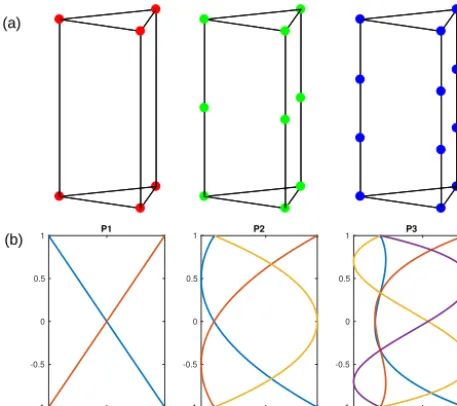
Figure 1.Panel(a): nodes for the P1×P1, P1×P2, and P1×P3
prismatic finite element. Panel(b): vertical nodal functions for P1,
P2, and P3 finite elements.
methods to improve runtime speed without sacrificing the models precision need to be addressed.
Here we present a method which builds upon the thermo-mechanical ice flow model ISSM to improve model speed within the BP ice sheet model simulations. While our imple-mentation and analysis are done with ISSM, the methods can be applied to a wide range of finite-element ice sheet models. The main component of this development focuses on the ver-tical extrusion of layers within ISSM and the type of finite elements used to create the vertical interpolation. The aim of this method is to allow the user to perform model sim-ulations that have a smaller number of vertical layers than typically used, while still being able to more precisely cap-ture the thermal state of the ice sheet than would otherwise be captured using traditional means of linear vertical interpola-tion. We begin by first describing the methodology associated with the implementation of higher-order vertical elements in Sect. 2, followed by a description of the model experiment setup for an idealized single-dome ice sheet and a realistic GrIS configuration in Sect. 3. The results are accompanied by a discussion in Sect. 4 and conclusions in Sect. 5.
2 Higher-order finite elements
Like many finite-element ice sheet models, ISSM relies on prismatic elements, which are the result of a vertical extru-sion of a two-dimenextru-sional triangular mesh. The interpolation used in these elements is decomposed into a horizontal in-terpolation and a vertical inin-terpolation. A P2×P1 finite ele-ment, for example, has a quadratic finite element on the hor-izontal plane (triangle) and a linear interpolation in the
ver-tical direction. Here, we assume that the variations in model fields are accurately captured by the horizontal mesh but that sharp gradients in the temperature at the base of the ice sheet need to be captured. For this purpose, we investigate finite el-ements that have three different degrees in the vertical nodal functions: (1) P1 linear elements, (2) P2, with a quadratic interpolation along thezaxis, and (3) P3, with a cubic inter-polation along thezaxis, as illustrated by Fig. 1.
Since the nodal functions are taken as a product of hor-izontal and vertical polynomials, they can be written in the following terms:Ni (x, y, z)=fj(x, y) × gk(z). Here, we
keep a linear interpolation for fj and they are classically
written as
f1(x, y)=x f2(x, y)=y
f3(x, y)=1−x−y (1)
in the standard triangle reference element whose corners are (0,0), (1,0), and (0,1). The functionsgk(z)control the degree
of interpolation along thez axis, and the nodes associated with these functions are located along the three vertical ments of the prism. The number of nodes along these seg-ments depends on the degree of these polynomials.
2.1 P1xP1 prismatic elements
In the vertical direction, we use a reference element that goes from z= −1 to z=1. A linear element (P1×P1; herein noted as P1) has six nodes: one per vertex. We have six nodal functions for the reference element, three in the horizontal plane (Eq. 1), times 2 along thezaxis:
g1(z)= 1
2(1−z) , g2(z)=
1
2(1+z). (2)
2.2 P1xP2 prismatic elements
For a quadratic finite element in the vertical direction (herein noted as P2), we have nine nodes per element (Fig. 1): one per vertex and one in the center of each vertical segment. We have the following functions in the vertical direction:
g1(z)= 1
2z(1−z), g2(z)= 1
2z (1+z) , g3(z)=
1−z2. (3)
2.3 P1xP3 prismatic elements
0 0.2 0.4 0.6 0.8 1 0
0.1 0.2 0.3 0.4 0.5 0.6 0.7 0.8 0.9 1
Exponential profile P1 interpolation P2 interpolation P3 interpolation
(a) (b)
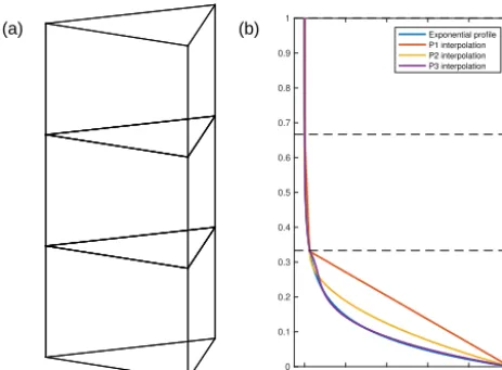
Figure 2.Panel (a) is an example of three prismatic elements used
to capture an exponential profile. Panel (b) is an example of
ex-ponential profile captured by P1, P2, and P3 finite elements. With higher-order finite elements in the vertical, sharp gradients in tem-perature are captured more precisely than with a linear (P1) inter-polation.
vertex and 2 located at one-third and two-thirds of each verti-cal segment. The vertiverti-cal components of the nodal functions are
g1(z)= − 9 16(z−1)
z−1
3 z+
1 3
,
g2(z)= 9 16
z−1
3 z+
1 3
(z+1),
g3(z)=27 16(z−1)
z−1 3
(z+1),
g4(z)= −27 16(z−1)
z+1 3
(z+1). (4)
2.4 Benefits of higher-order vertical finite elements Increasing the degree of finite elements along the zaxis is comparable to increasing the resolution along the z axis, whereby having higher-order polynomials makes it possible to better capture sharp changes despite the number of ele-ments in the vertical being limited to four or five. Figure 2 illustrates this idea for an exponential function that is repre-sentative of a thermal profile. Here, the ice is uniformly cold throughout except at the base where the ice is warmer due to the geothermal heat flux and frictional heating. Using only four layers and linear elements (P1), this vertical profile is poorly captured, as the number of layers is too small to cor-rectly represent the gradient of temperatures near the base. While quadratic elements do better, the cubic elements cap-ture the shape of the exponential curve with maximum accu-racy, even for a coarse mesh. For more information about the
finite-element method, we direct the reader to Zienkiewicz and Taylor (1989, 1991).
3 Model description and experimental setup
For the following model experiments we use the ISSM (Larour et al., 2012), a finite-element, thermomechanical ice sheet model. The tests performed in this study can be split into two experiments. We first test the precision of the higher-order vertical interpolation using a simplified single-dome ice sheet experiment that uses the SIA, following Experiment A of the European Ice Sheet Modeling INiTiative (EISMINT 2) experiments (Payne et al., 2000). We then apply a simi-lar setup to a GrIS-wide model, where the steady-state ther-mal solution is computed using the higher-order BP model. Specifics regarding model setup and the relevant experiments are discussed below.
3.1 Single-dome experiment setup
To test the performance of the higher-order vertical interpola-tion, we adopt a setup similar to the EISMINT 2 experiments (Payne et al., 2000), which were targeted for the assessment of thermomechanical shallow-ice models. We perform all of our single-ice-dome experiments using the SIA on models with a horizontal grid resolution of 20 km×20 km and with a model domain of 1500 km×1500 km. The maximum sur-face mass balance of 0.5 m yr−1 occurs at the center of the domain (over the dome summit) and linearly decreases ra-dially as a function of the geographical distance from the dome. Accordingly, the minimum surface air temperature (238.15 K) is set at the dome summit and decreases away from the dome following the same basis as the surface mass balance. The ice rheology is temperature dependent, follow-ing Cuffey and Paterson (2010, p. 75).
vertical interpolation, while the thermal computation makes use of the higher-order vertical elements.
3.2 GrIS model setup
In addition to comparison with the EISMINT 2 Experiment A, thermal steady-state computations are performed for a GrIS-wide model to determine how well the vertical interpo-lations can capture thermal profiles and basal temperatures throughout the ice sheet. The three-dimensional higher-order model (i.e., BP) of Blatter (1995) and Pattyn (2003) is used for the momentum balance equations. The nonlinear effec-tive ice viscosity results from Glen’s flow law (Glen, 1955) and is given in Eq. (5):
µ= B
2˙
n−1
n
e
, (5)
whereBis the ice hardness,nis the Glen’s flow law expo-nent, and˙eis the effective strain rate. The ice hardness,B, is temperature dependent following the rate factors given in Cuffey and Paterson (2010, p. 75), while basal drag is em-pirically determined following a viscous flow law outlined in Cuffey and Paterson (2010).
The GrIS-wide model relies on anisotropic mesh adapta-tion, whereby the element size is refined as a function of sur-face elevation (Howat et al., 2014) and InSAR (interferomet-ric synthetic-aperture radar) surface velocities from Rignot and Mouginot (2012), becoming finer in areas where the sec-ond derivative of these two quantities is higher. The model mesh has a horizontal resolution ranging from 3 km in areas of ice streams to 20 km over the interior regions where the ice flow is slow, corresponding to a two-dimensional model with ∼10 000 triangular elements. The horizontal mesh is then extruded to the corresponding number of layers outlined in Sect. 3.1. This results in 24 models with a 3-D mesh rang-ing from 30 000 to 100 000 prismatic elements, dependrang-ing on the model’s number of vertical elements. Similar to the ex-periments outlined in Sect. 3.1, we run a benchmark thermal steady-state simulation using a model that has 25 nonuni-form layers and uses the P1 vertical interpolation (250 000 elements).
The models are initialized with bed topography from Bed-Machine Greenland v3 (Morlighem et al., 2017) and ice sur-face elevation from the GMIP DEM (Greenland Mapping Project Digital Elevation Model) of Howat et al. (2014). The surface mass balance and surface temperatures are taken from Ettema et al. (2009), and the geothermal heat flux relies on a setup identical to Seroussi et al. (2013). The underly-ing geothermal heat flux from Shapiro and Ritzwoller (2004) is used; however, values of 20 and 60 mWm−2 are added at the Dye3 and GRIP sites, respectively, after Seroussi et al. (2013). These modifications follow an exponential decay from the particular sites with a radius of 250 km.
The thermal model for both the single-dome and steady-state experiments use an enthalpy formulation derived from
8p1 9p1
10p1
0 20 000 40 000 60 000 80 000 100 000
Time (yrs) 0 3 6 9 12 15 % . fr om 2 5 la ye r P1
0 20 000 40 000 60 000 80 000 100 000
Time (yrs) 0 3 6 9 12 15 % . fr om 2 5 la ye r P1 4p2 5p2 6p2 7p2 8p2 9p2 10p2 4p3 5p3 6p3 7p3 8p3 9p3 10p3
0 20000 40000 60000 80000 100000
Time (yrs) 0 3 6 9 12 15 % . fr om 2 5 la ye r P 1 (a) (b) (c)
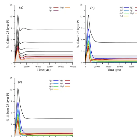
Figure 3.The percent difference in ice volume from the 25-layer
P1 model for models using the P1(a), P2(b), and P3(c)
verti-cal interpolation scheme over the 100 000-year relaxation. The gray shading highlights the models that fall within 2 % of the simulated ice volume for the 25-layer P1 model at the end of the 100 000-year relaxation. Only those models that fall within 2 % of the simulated ice volume for the 25-layer P1 model are labeled and colored as shown in their respective legends.
Aschwanden et al. (2012), which includes both temperate and cold ice. At the ice surface, air temperature is imposed, while the geothermal heat flux is applied at the base. For full details outlining the thermal model used in ISSM, we direct the reader to Seroussi et al. (2013) and Larour et al. (2012). Lastly, the spatially varying basal drag coefficient is deter-mined using inverse methods (Morlighem et al., 2010; Larour et al., 2012), providing the best match between modeled and InSAR surface velocities from Rignot and Mouginot (2012).
4 Results and discussion 4.1 Single-dome experiment
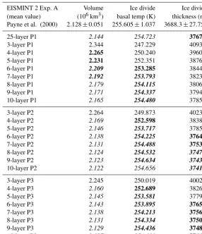
Table 1.Ice volume, ice divide basal temperature, and ice divide thickness for each individual simulation after a 100 kyr relaxation. Also shown are the corresponding mean values for the EISMINT 2 (Payne et al., 2000) Experiment A simulation and the standard deviation. Those values that fall within 1 standard deviation from the EISMINT 2 Experiment A mean values are given in italics, those within 2 standard deviations in bold italics and those within 3 standard deviations in bold.
EISMINT 2 Exp. A Volume Ice divide Ice divide
(mean value) (106km3) basal temp (K) thickness (m)
Payne et al. (2000) 2.128±0.051 255.605±1.037 3688.3±27.757
25-layer P1 2.144 254.723 3767.0
3-layer P1 2.344 247.229 4093.2
4-layer P1 2.265 250.240 3960.4
5-layer P1 2.231 252.351 3876.5
6-layer P1 2.209 253.285 3844.4
7-layer P1 2.192 253.793 3823.0
8-layer P1 2.179 254.115 3806.7
9-layer P1 2.171 254.337 3794.5
10-layer P1 2.165 254.480 3785.4
3-layer P2 2.264 249.873 4023.2
4-layer P2 2.169 252.598 3838.1
5-layer P2 2.146 253.717 3785.8
6-layer P2 2.138 254.225 3764.8
7-layer P2 2.131 254.488 3753.9
8-layer P2 2.124 254.532 3747.1
9-layer P2 2.123 254.634 3743.6
10-layer P2 2.122 254.656 3741.3
3-layer P3 2.245 250.019 4002.0
4-layer P3 2.160 252.689 3826.4
5-layer P3 2.145 253.581 3779.3
6-layer P3 2.143 253.895 3765.0
7-layer P3 2.138 254.213 3756.5
8-layer P3 2.131 254.334 3750.3
9-layer P3 2.129 254.436 3748.5
10-layer P3 2.127 254.600 3746.2
(P1) interpolation (Fig. 3a) is used in the thermal model, only those models with at least 8 layers fall within the 2 % range of ending ice volume for the 25-layer P1 simulation. When using a higher-order vertical interpolation (P2 and P3), how-ever, models with four layers and above fall within the 2 % range (Fig. 3b and c).
To further compare the performance of each model, the corresponding ice volume, ice divide basal temperature, and ice divide thickness are shown in Table 1 for each model sim-ulation and are compared to the mean values derived from the EISMINT 2 Experiment A results (Payne et al., 2000). It is important to note that no known analytic solution was provided in the EISMINT 2 Experiment A comparison. Sim-ilar to Rutt et al. (2009), however, we compare our simulated values to the mean and the standard deviation of the values for Experiment A in the EISMINT 2 experiments to assess the relative spread. In general, models using the higher-order vertical interpolation tend to better match the EISMINT 2 re-sults. Models with four layers or more using the P2 or P3 vertical interpolation fall within 1 standard deviation (σ )of
the mean for simulated ice volume, whereas models using the linear vertical interpolation require eight or more layers to satisfy this constraint. With respect to the basal tempera-tures simulated at the ice divide, only the layer P2, 10-layer P3, and the 25-10-layer P1 simulations fall within 1σ of the mean for the EISMINT 2 Experiment A results.
temper-3 4 5 6 7 8 9 10 Number of layers
-2 0 2 4 6 8 10
%
-fr
om
2
5-la
ye
r
P1
f
in
al
v
ol
um
e
P1 P2 P3
Figure 4.The percent difference in simulated ice volume after the 100 000-year relaxation for the single-ice-dome experiment com-pared to the 25-layer P1 model. Each model run is shown as a func-tion of the vertical interpolafunc-tion and the number of layers used.
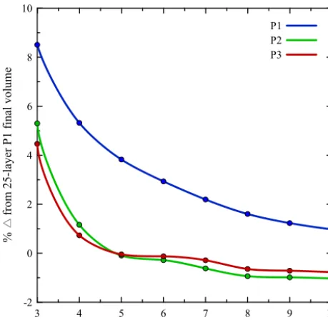
atures simulated with the P2 interpolation, which may feed back onto the ice rheology and, correspondingly, the ice flow. We note however that these differences are small, and over-all models using the P2 and P3 vertical interpolation show excellent agreement amongst each other. From this exercise, it can be concluded that when using fewer layers, models that utilize the higher-order vertical interpolation are more capable of capturing the simulated ice volume, ice divide basal temperatures, and ice divide thickness simulated by the EISMINT 2 Experiment A models. Although some differ-ences do exist between our simulated values and those de-rived from the EISMINT 2 Experiment A results, the preci-sion of the models using the P2 or P3 vertical interpolation is reasonable. As noted by Rutt et al. (2009), there are inherent difficulties in associating particular differences with specific model processes. Most differences in the simulated tempera-ture can have feedbacks on the ice rheology and therefore the ice flow, which makes comparisons with models using dif-ferent discretization methods difficult. Overall, comparison with the EISMINT 2 Experiment A results demonstrate that by using fewer layers with a higher-order vertical interpola-tion, models are capable of capturing particular constraints more accurately than would otherwise be simulated using a linear vertical interpolation.
Because of the potential difficulties in assessing differ-ences between our results and those derived from the EIS-MINT 2 Experiment A, we also compare our results to the model simulation using the 25-layer P1 vertical interpola-tion. Because this model is representative of what is
char-Table 2.The absolute value of the percent difference between each individual model run and the 25-layer P1 simulation at the end of the 100 000-year relaxation for ice volume, ice divide basal temper-ature, and ice divide thickness. Italics denote models that fall within 1 % of the variables simulated by the 25-layer P1 model at the end of the relaxation.
Ice Ice divide Ice divide
volume basal temp. thickness
3-layer P1 9.33 2.94 8.66
4-layer P1 5.64 1.76 5.13
5-layer P1 4.06 0.93 2.91
6-layer P1 3.03 0.56 2.05
7-layer P1 2.24 0.37 1.49
8-layer P1 1.63 0.24 1.05
9-layer P1 1.26 0.15 0.73
10-layer P1 0.98 0.10 0.49
3-layer P2 5.60 1.90 6.80
4-layer P2 1.17 0.83 1.89
5-layer P2 0.09 0.39 0.50
6-layer P2 0.28 0.20 0.06
7-layer P2 0.61 0.09 0.35
8-layer P2 0.93 0.08 0.53
9-layer P2 0.95 0.04 0.62
10-layer P2 0.98 0.03 0.68
3-layer P3 4.71 1.85 6.24
4-layer P3 0.75 0.80 1.58
5-layer P3 0.05 0.45 0.33
6-layer P3 0.05 0.33 0.05
7-layer P3 0.28 0.20 0.28
8-layer P3 0.61 0.15 0.44
9-layer P3 0.70 0.11 0.49
10-layer P3 0.79 0.05 0.55
-35 -25 -15 Temperature ( C)
3 layers 5 layers 7 layers 25 layers P1
-35 -25 -15
Temperature ( C) 0
500 1000 1500 2000 2500 3000 3500 4000
E
le
va
ti
on
(
m
)
P1 P2
-35 -25 -15
Temperature ( C)
P3 Ice divide temperature profile for the relaxed SIA circular ice sheet
Figure 5.The resulting temperature profiles at the ice divide after the 100 000-year single-ice-dome relaxation for models with 3, 5, and 7 layers, compared to the temperature profile from the 25-layer P1 model.
P1 model is shown as a function of the number of layers in each model. Those models using the P2 and P3 vertical in-terpolation converge significantly faster to ∼0–1 % differ-ence at 4–5 layers than the 25-layer P1 model. We note that the negative difference for the P2 and P3 models arises as the temperatures simulated with the higher-order vertical in-terpolation are slightly higher but not significantly different than that simulated by the 25-layer P1 model (Table 2), pro-viding a feedback between ice rheology and ice flow. Lastly, the ice divide thickness follows a similar trend in that using the higher-order vertical interpolation allows a model with fewer layers to capture what is simulated with the 25-layer P1 model (Table 2). When viewed as ice profiles extending from the dome summit to the ice edge for three-, five-, and seven-layer models (Fig. S1 in the Supplement), the differ-ences in ice thickness between models appear small, with the P2 and P3 being almost identical and only minor differences existing for the models using the P1 vertical interpolation.
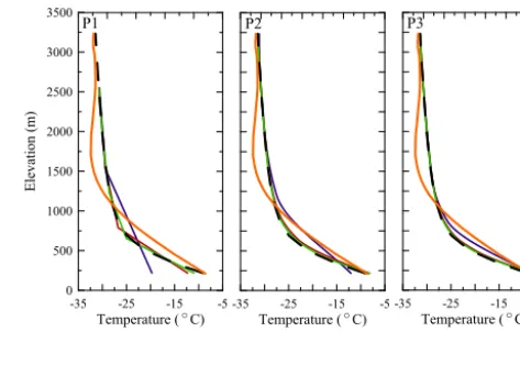
Differences between the linear vertical interpolation and the P2 or P3 interpolation become more apparent when ana-lyzing ice temperature profiles. In Fig. 5, ice temperature pro-files are plotted at the ice divide for models with three, five, and seven layers. With only three layers, models with the P1, P2, and P3 vertical interpolation simulate a temperature pro-file that is too warm between 500 and 1500 m and too cold approaching the base. Despite the vertical interpolation used, the profile is not well captured, although improvements to the shape of the temperature profile in the transition between 500 and 1500 m can be seen in models using the higher-order vertical interpolation. Adding more layers to each model im-proves the overall fit to the 25-layer P1 model, although the models using the P2 and P3 vertical interpolation capture the shape of the temperature profile much better than the linear interpolation. The overall fit is improved not only at the base
Figure 6.Run times for the 100-year higher-order simulation of the single ice dome for each individual model based upon the number of layers and the vertical interpolation scheme used.
but also in the transition between 500 and 1500 m where the ice begins to warm more rapidly approaching the base. We also find that the differences between the P2 and P3 verti-cal interpolation are marginal in this example, indicating that using a quadratic vertical interpolation (P2) is suitable when given the choice to use a cubic vertical interpolation (P3).
4.2 Improvements in simulation speed
Although much of the success regarding the higher-order ver-tical interpolation resides in the model’s ability to capture the vertical structure of temperature in the ice using fewer layers than is needed from the traditional linear vertical in-terpolation, improvements to model speed are the main moti-vation for its implementation, particularly in BP models. To test how model speed is improved when implementing the higher-order vertical interpolation, we begin by using the re-laxed model simulations that have thus far only used the SIA for the single-dome experiments in Sect. 4.1. From the re-laxed model states, each simulation is run for 100 years using the BP ice flow model in ISSM and using the same bound-ary conditions from the relaxation with a fixed time step of 0.2 years.
inter-polation used, complete the 100-year run anywhere between 241 (3P1) and 9 (10P3) times faster (Fig. 6). To determine how models perform based upon the vertical interpolation, a criterion is established based upon Table 2, such that each model’s simulated ice volume must be within 1 % of those values simulated by the 25-layer P1 model, which represents the relative uncertainty associated with the present-day ice volume of the GrIS (Morlighem et al., 2017). Based upon these criteria, models using the P1 vertical interpolation must have 10 layers or more, while models using the P2 and P3 vertical interpolation can use at least 5 or 4 layers, respec-tively. When applying these criteria, runtime is 5 times faster for a 5-layer P2 model versus a 10-layer P1 model. If we as-sume a seven-layer P1 model is adequate, the runtime for a five-layer P2 model is 2 times faster. When compared with the 25-layer P1 model, the 5-layer P2 model completes the relaxation 57 times faster.
4.3 Application to a GrIS-wide model
The thermal steady-state simulation is compared with the GRIP ice core record (Dahl-Jensen et al., 1998) in Fig. 7 for models with 3, 5, and 7 layers as well as the 25-layer model with the P1 vertical interpolation. The simulated thermal structure for the 25-layer P1 model is similar to the thermal profile presented in Seroussi et al. (2013). Temperature dif-ferences of 2–5◦C occur between the models and the GRIP record between 1200 and 2200 m and 500 and 1000 m; how-ever, this is consistent with other models computing the ther-mal steady state (Dahl-Jensen et al., 1998; Rogozhina et al., 2011). The influence of past surface temperatures, ice flow history, and accumulation are not represented in our thermal steady-state computation. Spinning up an ice sheet model over a glacial cycle typically provides a better match to the ice core records but is beyond the scope of this experiment (Greve, 1997; Rogozhina et al., 2011). Nevertheless, the gen-eral profile is well simulated, with only minor differences in the simulated basal temperatures for the models using P2 or P3 interpolations. Similar to the results presented for the ice dome (Fig. 5), models using the higher-order vertical inter-polation simulate the shape of the thermal profile (compared to 25-layer P1) much better than the models using the linear vertical interpolation and the same number of layers. When examined spatially, the difference in basal temperature de-creases using a model with a higher-order vertical interpola-tion, particularly over the interior of the ice sheet (Fig. S2a– c). Although differences between models using the P1 verti-cal interpolation and the 25-layer model begin to minimize with 8 layers, the differences for models using the P2 and P3 vertical interpolation become small with 4–5 layers.
-35 -25 -15 -5
Temperature ( C)
0 500 1000 1500 2000 2500 3000 3500
E
le
va
tio
n
(m
)
-35 -25 -15 -5
Temperature ( C)
25 P1 3 layers 5 layers 7 layers GRIP
P1 P2
-35 -25 -15 -5
Temperature ( C)
P3
Figure 7.The resulting temperature profiles for the higher-order steady-state thermal computation at the GRIP ice core site location for models with 3, 5, and 7 layers, compared to the temperature pro-file from the 25-layer P1 model and the measured GRIP temperature profile (Dahl-Jensen et al., 1998).
5 Conclusions
This study aims at addressing the current computational lim-itation in using higher-order stress balance ice sheet mod-els for paleoclimate studies. Currently, analysis of ice sheet modeling experiments focusing on the past behavior of the GrIS is being complemented with rich paleoclimate data-constraining features of the past ice sheet behavior (Larsen et al., 2015; Young and Briner, 2015; Sinclair et al., 2016). Where shallow-ice models might be limited in their ability to simulate the marginal behavior of the GrIS through the ex-clusion of higher-order stress terms and an inability to run on a high-resolution mesh, BP models may become more ap-propriate for such comparisons in the future. To help alleviate the computational expense in using a BP model, we imple-ment higher-order vertical eleimple-ments. As shown in Sect. 4.1 of this study, increasing the degree of the vertical interpolation allows the model to capture gradients in the thermal profile of the ice with more precision than would otherwise be cap-tured using a model with a linear vertical interpolation, de-spite having the same number of vertical layers. Models with correspondingly fewer layers that used the higher-order ver-tical interpolation were able to capture the transient behavior consistent with the EISMINT 2 Experiment A results (Payne et al., 2000) and also performed well when compared to a model similar to those that are used for modeling studies in ISSM (Seroussi et al., 2013).
using the higher-order vertical interpolation were shown to shorten runtime anywhere between 2 and 5 times for a 5-layer model compared to models with 7 and 10 5-layers, re-spectively, using a linear vertical interpolation. When com-pared to the 25-layer model using the linear vertical inter-polation, models with 5 to 10 layers using the higher-order vertical interpolation had anywhere between a 57 to 10 times faster runtime, with minimal impacts on the precision of the simulated ice volume and thermal state. When the higher-order vertical elements were applied to a three-dimensional, BP model of the GrIS, experiments showed the thermal state of the ice sheet can be captured as precisely as our 25-layer P1 model when at least 5 layers are used for a quadratic (P2) vertical interpolation and at least 4 layers for a cubic (P3) vertical interpolation. When comparing the quadratic and cu-bic vertical interpolation, the benefits of using a cucu-bic verti-cal interpolation are slight, although it may be useful when modeling in areas of complex thermal regimes.
In the context of paleoclimate simulations, using a higher-order vertical interpolation improves simulation speed, par-ticularly for BP ice sheet models. BP models using this will still likely be too computationally intensive for simulations which sample parameter space and thus require multiple in-dependent simulations (Applegate et al., 2012; Robinson et al., 2011). However, in experiments where BP models may offer improvements in model data comparison versus using shallow-ice models, higher-order vertical elements can be used as a means to improve model speed while still being able to capture the qualities simulated in a model with many more layers but at the fraction of the speed. In this respect, future studies will use these higher-order vertical elements to enhance computational speed while maintaining mechanical complexity for ice sheet modeling experiments over various paleoclimate timescales.
Code availability. The higher-order finite elements are currently implemented in the ISSM code, which can be compiled follow-ing the instructions on the ISSM website (https://issm.jpl.nasa.gov/ download, last access: 3 March 2018).
Supplement. The supplement related to this article is available online at: https://doi.org/10.5194/gmd-11-1683-2018-supplement.
Competing interests. The authors declare that they have no conflict of interest.
Edited by: Jeremy Fyke
Reviewed by: two anonymous referees
References
Alley, R. B., Andrews, J. T., Miller, G. H., White, J. W. C., Brigham-Grette, J., Clarke, G. K. C., Cuffey, K. M., Fitzpatrick, J. J., Muhs, D. R., Funder, S., Marshall, S. J., Mitrovica, J. X., Otto-Bliesner, B. L., and Polyak, L.: History of the Greenland Ice Sheet: Paleoclimatic insights, Quatern. Sci. Rev., 29, 1728–1756, https://doi.org/10.1016/j.quascirev.2010.02.007, 2010.
Applegate, P. J., Kirchner, N., Stone, E. J., Keller, K., and Greve, R.: An assessment of key model parametric uncertainties in projec-tions of Greenland Ice Sheet behavior, The Cryosphere, 6, 589– 606, https://doi.org/10.5194/tc-6-589-2012, 2012.
Aschwanden, A., Bueler, E., Khroulev, C., and Blatter, H.: An en-thalpy formulation for glaciers and ice sheets, J. Glaciol., 58, 441–457, https://doi.org/10.3189/2012JoG11J088, 2012. Aschwanden, A., Fahnestock, M. A., and Truffer, M.: Complex
Greenland outlet glacier flow captured, Nat. Commun., 7, 10524, https://doi.org/10.1038/ncomms10524, 2016.
Blatter, H.: Velocity and stress-fields in grounded glaciers: A simple algorithm for including deviatoric stress gradients, J. Glaciol.,
41, 333–344, https://doi.org/10.3189/S002214300001621X,
1995.
Briner, J. P., McKay, N. P., Axford, Y., Bennike, O., Bradley, R. S., de Vernal, A., Fisher, D., Francus, P., Fréchette, B., Gajew-ski, K., Jennings, A., Kaufman, D. S., Miller, G. H., Rous-ton, C., and Wagner, B.: Holocene climate change in Arc-tic Canada and Greenland, Quatern. Sci. Rev., 147, 340–364, https://doi.org/10.1016/j.quascirev.2016.02.010, 2016.
Bueler, E., Lingle, C. S., KallenBrown, J. A., Covey, D. N., and Bowman, L. N.: Exact solutions and verification of numeri-cal models for isothermal ice sheets, J. Glaciol., 51, 291–306, https://doi.org/10.3189/172756505781829449, 2005.
Bueler, E. and Brown, J.: Shallow shelf approximation as a “sliding law” in a thermomechanically coupled ice sheet model, J. Geo-phys. Res., 114, F03008, https://doi.org/10.1029/2008JF001179, 2009.
Church, J. A., Clark, P. U., Cazenave, A., Gregory, J. M., Jevrejeva, S., Levermann, A., Merrifield, M. A., Milne, G. A., Nerem, R. S., Nunn, P. D., Payne, A. J., Pfeffer, W. T., Stammer, D., and Un-nikrishnan, A. S.: Sea Level Change. In: Climate Change 2013: The Physical Science Basis, Contribution of Working Group I to the Fifth Assessment Report of the Intergovernmental Panel on Climate Change, edited by: Stocker, T. F., Qin, D., Plattner, G.-K., Tignor, M., Allen, S. G.-K., Boschung, J., Nauels, A., Xia, Y., Bex, V., and Midgley, P. M., Cambridge University Press, Cam-bridge, United Kingdom and New York, NY, USA, 2013. Cuffey, K. M. and Paterson, W. S. B.: The physics of glaciers, 4th
Edn., Butterworth-Heinemann, Oxford, 2010.
Dahl-Jensen, D., Mosegaard, K., Gundestrup, G., Clow, G. D., Johnsen, S. J., Hansen, A. W., and Balling, N.: Past temperatures directly from the Greenland ice sheet, Science, 282, 268–271, https://doi.org/10.1126/science.282.5387.268, 1998.
Ettema, J., van den Broeke, M. R., van Meijgaard, E., van de Berg, W. J., Bamber, J. L., Box, J. E., and Bales, R. C.: Higher surface mass balance of the Greenland Ice Sheet revealed by high-resolution climate modeling, Geophys. Res. Lett., 36, 1–5, https://doi.org/10.1029/2009GL038110, 2009.
of the Greenland ice sheet, The Cryosphere, 7, 183–199, https://doi.org/10.5194/tc-7-183-2013, 2013.
Glen, J. W.: The creep of polycrystalline ice, Proc. R. Soc. London, Ser. A, 228, 519–538, https://doi.org/10.1098/rspa.1955.0066, 1955.
Greve, R.: Application of a polythermal three-dimensional ice sheet model to the Greenland ice sheet: response
to steady-state and transient climate scenarios, J.
Climate, 10, 901–918,
https://doi.org/10.1175/1520-0442(1997)010<0901:AOAPTD>2.0.CO;2, 1997.
Greve, R., Saito, F., and Abe-Ouchi, A.: Initial results of the SeaRISE numerical experiments with the models SICOPOLIS and IcIES for the Greenland Ice Sheet, Ann. Glaciol., 52, 23–30, https://doi.org/10.3189/172756411797252068, 2011.
Howat, I. M., Negrete, A., and Smith, B. E.: The Green-land Ice Mapping Project (GIMP) Green-land classification and surface elevation data sets, The Cryosphere, 8, 1509–1518, https://doi.org/10.5194/tc-8-1509-2014, 2014.
Hutter, K.: Theoretical Glaciology: Material Science of Ice and the Mechanics of Glaciers and Ice Sheets, D. Reidel, Dordrecht, Netherlands, 1983.
Huybrechts, P.: Sea-level changes at the LGM from ice-dynamic reconstructions of the Greenland and Antarctic ice sheets during the glacial cycles, Quatern. Sci. Rev., 21, 203–231, 2002. Kirchner, N., Hutter, K., Jakobsson, M., and Gyllencreutz, R.:
Ca-pabilities and limitations of numerical ice sheet models: a dis-cussion for Earth-scientists and modelers, Quatern. Sci. Rev., 30, 3691–3704, https://doi.org/10.1016/j.quascirev.2011.09.012, 2011.
Larour, E., Seroussi, H., Morlighem, M., and Rignot, E.: Continen-tal scale, high order, high spatial resolution, ice sheet modeling using the Ice Sheet System Model (ISSM), J. Geophys. Res., 117, F01022, https://doi.org/10.1029/2011JF002140, 2012.
Larsen, N., Kjaer, K., Lecavalier, B., Bjork, A., Colding, S., Huy-brechts, P., Jakobsen, K., Kjeldsen, K., Knudsen, K., Odgaard, B., and Olsen, J.: The response of the southern Greenland ice sheet to the Holocene thermal maximum, Geology (Boulder Colo.), 43, 291–294, https://doi.org/10.1130/G36476.1, 2015 Lecavalier, B. S., Milne, G. A., Simpson, M. J. R., Wake, L.,
Huy-brechts, P., Tarasov, L., Kjeldsen, K. K., Funder, S., Long, A. J., Woodroffe, S., Dyke, A. S., and Larsen, N. K.: A model of Greenland ice sheet deglaciation constrained by observations of relative sea level and ice extent, Quatern. Sci. Rev., 102, 54–84, https://doi.org/10.1016/j.quascirev.2014.07.018, 2014.
MacAyeal, D. R.: Large-scale ice flow over a viscous
basal sediment: theory and application to Ice Stream
B, Antarctica, J. Geophys. Res., 94, 4071–4087,
https://doi.org/10.1029/JB094iB04p04071, 1989.
Morlighem, M., Rignot, E., Seroussi, H., Larour, E., Ben Dhia, H., and Aubry, D.: Spatial patterns of basal drag inferred using con-trol methods from a full-Stokes and simpler models for Pine Is-land Glacier, West Antarctica, Geophys. Res. Lett., 37, L14502, https://doi.org/10.1029/2010GL043853, 2010.
Morlighem, M., Williams, C. N., Rignot, E., An, L., Arndt, J. E., Bamber, J. L., Catania, G., Chauché, N., Dowdeswell, J. A., Dorschel, B., Fenty, I., Hogan, K., Howat, I., Hubbard, A., Jakob-sson, M., Jordan, T. M., Kjeldsen, K. K., Millan, R., Mayer, L., Mouginot, J., Noël, B. P. Y., Cofaigh, C. Ó, Palmer, S., Rys-gaard, S., Seroussi, H., Siegert, M. J., Slabon, P., Straneo, F., van
den Broeke, M. R., Weinrebe, W., Wood, M., and Zinglersen, K. B.: BedMachine v3: Complete bed topography and ocean bathymetry mapping of Greenland from multi-beam echo sound-ing combined with mass conservation, Geophys. Res. Lett., 44, 11051–11061, https://doi.org/10.1002/2017GL074954, 2017. Pattyn, F.: A new three-dimensional higher-order
thermomechani-cal ice sheet model: Basic sensitivity, ice stream development, and ice flow across subglacial lakes, J. Geophys. Res., 108, 2382, https://doi.org/10.1029/2002JB002329, 2003.
Payne, A. J., Huybrechts, P., Abe-Ouchi, A., Calov, R., Fastook, J. L., Greve, R., Marshall, S. J., Marsiat, I., Ritz, C., Tarasov, L., and Thomassen, M. P. A.: Results from the EISMINT model intercomparison: the effects of thermomechanical coupling, J. Glaciol., 46, 227–238, 2000.
Pollard, D. and Deconto, R. M.: Modelling West Antarctica ice sheet growth and collapse through the past five million years, Na-ture, 458, 329–332, https://doi.org/10.1038/nature07809, 2009. Rignot, E. and Mouginot, J.: Ice flow in Greenland for the
interna-tional polar year 2008–2009, Geophys. Res. Lett., 39, L11501, https://doi.org/10.1029/2012GL051634, 2012.
Robinson, A., Calov, R., and Ganopolski, A.: Greenland ice sheet model parameters constrained using simulations of the Eemian Interglacial, Clim. Past, 7, 381–396, https://doi.org/10.5194/cp-7-381-2011, 2011.
Rogozhina, I., Martinec, Z., Hagedoorn, J. M., Thomas,
M., and Fleming, K.: On the long-term memory of the
Greenland Ice Sheet, J. Geophys. Res., 116, F01011,
https://doi.org/10.1029/2010JF001787, 2011.
Rutt, I. C., Hagdorn, M., Hulton, N. R. J., and Payne, A. J.: The Glimmer community ice sheet model, J. Geophys. Res.-Earth
Surf., 114, F02004, https://doi.org/10.1029/2008JF001015,
2009.
Seddik, H., Greve, R., Zwinger, T., Gillet-Chaulet, F., and Gagliar-dini, O.: Simulations of the Greenland ice sheet 100 years into the future with the full Stokes model Elmer/Ice, J. Glaciol., 58, 427–440, https://doi.org/10.3189/2012JoG11J177, 2012. Seddik, H., Greve, R., Zwinger, T., and Sugiyama, S.: Regional
modeling of the Shirase drainage basin, East Antarctica: full Stokes vs. shallow ice dynamics, The Cryosphere, 11, 2213– 2229, https://doi.org/10.5194/tc-11-2213-2017, 2017.
Seroussi, H., Morlighem, M., Rignot, E., Khazendar, A., Larour, E., and Mouginot, J.: Dependence of greenland ice sheet projections on its thermal regime, J. Glaciol., 59, 218, https://doi.org/10.3189/2013JoG13J054, 2013.
Shapiro, N. M. and Ritzwoller, M. H.: Inferring surface heat flux distribution guided by a global seismic model: particular ap-plication to Antarctica, Earth Planet. Sci. Lett., 223, 213–224, https://doi.org/10.1016/j.epsl.2004.04.011, 2004.
Sinclair, G., Carlson, A. E., Mix, A. C., Lecavalier, B. S., Milne, G., Mathias, A., Buizert, C., and Deconto, R.: Diachronous retreat of the Greenland ice sheet dur-ing the last deglaciation, Quatern. Sci. Rev., 145, 243–258, https://doi.org/10.1016/j.quascirev.2016.05.040, 2016.
Tarasov, L. and Richard Peltier, W.: Greenland glacial history and local geodynamic consequences, Geophys. J. Int., 150, 198–229, https://doi.org/10.1046/j.1365-246X.2002.01702.x, 2002. Young, N. E. and Briner, J. P.: Holocene evolution of
the western Greenland Ice Sheet: assessing
geophys-ical ice-sheet models with geological reconstructions
of ice-margin change, Quatern. Sci. Rev., 114, 1–17,
https://doi.org/10.1016/j.quascirev.2015.01.018, 2015.
Zienkiewicz, O. C. and Taylor, R. L.: The finite element method, Vol. I. Basic formulations and linear problems. London: McGraw-Hill, London: McGraw-Hill, p. 648, [School of Engi-neering, University of Wales. Swansea, Wales], 1989.