A new approach to the intracardiac
inverse problem using Laplacian distance kernel
Raúl Caulier‑Cisterna
1, Sergio Muñoz‑Romero
1,2, Margarita Sanromán‑Junquera
1, Arcadi García‑Alberola
3and José Luis Rojo‑Álvarez
1,2*Background
Cardiac arrhythmias are often first detected with electrocardiogram (ECG) monitoring, which consists of recording the electrical potential produced by the heart in the skin [1]. ECG interpretation is crucial for arrhythmia diagnosis, and in recent years, different techniques have been studied to improve the ECG signal quality, including the search for new materials for the electrodes [2], the design of cardiac monitoring systems [3, 4] combining the analysis of ECG signals and other non-invasive signals such as the seis-mocardiogram [5], the estimation of fetal ECG [6], the impact of noise and improvement
Abstract
Background: The inverse problem in electrophysiology consists of the accurate estimation of the intracardiac electrical sources from a reduced set of electrodes at short distances and from outside the heart. This estimation can provide an image with relevant knowledge on arrhythmia mechanisms for the clinical practice. Methods based on truncated singular value decomposition (TSVD) and regularized least squares require a matrix inversion, which limits their resolution due to the unavoidable low‑ pass filter effect of the Tikhonov regularization techniques.
Methods: We propose to use, for the first time, a Mercer’s kernel given by the Lapla‑ cian of the distance in the quasielectrostatic field equations, hence providing a Sup‑ port Vector Regression (SVR) formulation by following the principles of the Dual Signal Model (DSM) principles for creating kernel algorithms.
Results: Simulations in one‑ and two‑dimensional models show the performance of our Laplacian distance kernel technique versus several conventional methods. Firstly, the one‑dimensional model is adjusted for yielding recorded electrograms, similar to the ones that are usually observed in electrophysiological studies, and suitable strategy is designed for the free‑parameter search. Secondly, simulations both in one‑ and two‑ dimensional models show larger noise sensitivity in the estimated transfer matrix than in the observation measurements, and DSM−SVR is shown to be more robust to noisy transfer matrix than TSVD.
Conclusion: These results suggest that our proposed DSM−SVR with Laplacian distance kernel can be an efficient alternative to improve the resolution in current and emerging intracardiac imaging systems.
Keywords: Inverse problem, Electrophysiology, Mercer’s kernel, Laplacian, Support Vector Regression, Dual Signal Model
Open Access
© The Author(s) 2018. This article is distributed under the terms of the Creative Commons Attribution 4.0 International License
(http://creat iveco mmons .org/licen ses/by/4.0/), which permits unrestricted use, distribution, and reproduction in any medium,
provided you give appropriate credit to the original author(s) and the source, provide a link to the Creative Commons license, and indicate if changes were made. The Creative Commons Public Domain Dedication waiver (http://creat iveco mmons .org/publi cdoma in/zero/1.0/) applies to the data made available in this article, unless otherwise stated.
RESEARCH
*Correspondence: joseluis.rojo@urjc.es
1 Department of Signal
Theory and Communications and Telematics
and Computation, Rey Juan Carlos University, Camino del Molino s/n, 28943 Fuenlabrada, Madrid, Spain
The electrical source estimation from regularized inversions is an ill-posed problem, thus different approaches have been proposed to deal with it [23–27]. Most of the pro-posed algorithms, including the truncated singular value decomposition (TSVD), the regularized Least Squares (LS), the curvature of the L-curve from Tikhonov method, and the minimum relative entropy, perform the inversion of the transfer matrix of the problem, which causes resolution reduction to their solutions [28–30]. The inverse prob-lem has been deeply studied in many other applications, but in the case of the inverse problem in electrophysiology, the transfer matrix can be either structurally simple and only depend on the distance, or structurally more complex and include spatial informa-tion, such as the torso-organ geometries and conductivities [31–33].
In the last years, Support Vector Machines (SVMs) and kernel methods have been proposed for a variety of applications, mainly for classification and regression schemes [34–37]. Sometimes the Support Vector Regression (SVR) algorithm has been straight-forwardly used to address signal processing problems on a straightforward way, this is, with little or no modification of the SVR algorithms to adapt the underlying data struc-ture from the rich available set of signal models. Whereas this has been an advantageous approach, often the performance is affected for this algorithm mismatching to the prob-lem. In [38], an approximation was proposed for tackling estimation problems in digital signal processing using SVMs, where a methodology to establish non-linear estimation of problems was proposed, so-called the Dual Signal Model (DSM) method, by follow-ing a similar methodology to previous SVM works addressfollow-ing sparse deconvolution and non-uniform interpolation [39, 40],
In this paper, we propose to create a SVR algorithm explicitly accounting for the sin-gularities of the data model, the physical equations and the constrains of the inverse problem in electrophysiology. For this purpose, the so-called Laplacian distance kernel is proposed for its use as Mercer’s kernel in the SVR, and the DSM is followed to create this algorithm ensuring its suitability as a single-minimum method. In general, all the statistical learning methods based on SVR have been shown to exhibit excellent regu-larization properties, and moreover, they allow us to readily introduce relevant a priori
information of the problem at hand into the algorithm equations, which is a desirable advantage for this novel application.
In the current approach, we have addressed a highly simplified model problem, whereas current literature is widely devoted to more complex and realistic geometries. Nevertheless, several resolution and accuracy issues remain present in current systems, which justifies the search for new approaches starting from the very principles. It can be expected that the limitations in the regularization models used so far in the inverse problem in electrophysiology will be overcome by the deep knowledge developed in the kernel-method field during the last years, as far as the bioelectric models are ration-ally included in the kernel equations. On the other hand, we propose the adaptation of the non-linear DSM for SVR (DSM−SVR) algorithm to the inverse problem in
distance between the catheters and the cardiac tissue in the quasielectrostatic field equa-tions. This kernel is used for the first time in the DSM−SVR algorithm, overall yielding a new algorithm for the inverse problem in electrophysiology.
The scheme rest of the paper is as follows. In Section II, the basic physical equations of a one- and two-dimensional model and the equations of the catchment model are intro-duced and the most usual algorithms used for the solution of the inverse problem and the DSM−SVR algorithm are also described. In Section III, results of the DSM−SVR algorithm in synthetic experiments using one- and two-dimensional models are bench-marked versus several usual algorithms. Special attention is devoted in the experiments to the effect of introducing noise in the transfer matrix instead of in the observed EGMs, which evidences the robustness of the SVM-DSP proposed algorithm. Finally, Section IV summarizes the discussion and the conclusions of the work.
Problem formulation and methods
There exists a gap between the literature of the inverse problem in electrophysiology and the clinical obtention and use of the estimated potentials. On the one hand, the inverse problem in cardiology and in electrophysiology usually aims to estimate the measured bioelectric potential at a given anatomical point (or set of points), which is considered as equivalent to measure the potential with a unipolar electrode. Nevertheless, it is well known that the measured potential by an electrode is due to the mixed contributions of the transmembrane action potentials. Ideally, the determination of the transmembrane action potential would give the best clinical information to the electrophysiologist, hence providing a pure electrical activity and view of the arrhythmia mechanism. However, this problem has been often limited to detailed in-silico models, in which the cellular activa-tion is generated, and then the obtained virtual potential electrograms are calculated. For this reason, we decided to work with a computational model generating the measurements in terms of the transmembrane action potentials, as this approach has been widely vali-dated in previous works [see e.g., [41–43], despite being still far from the clinical practice.
This section describes the equations of the quasielectrostatic model used to formulate the forward problem in electrophysiology, and a simple demonstration of its expression as a Linear and Space Invariant System (LSIS) relating two multidimensional spatial sig-nals, namely, the transmembrane potential and the extracellular potential. In order to work with this LSIS model, we implement traditional solutions to the inverse problem, including Tikhonov regularization [44–46], the modified TSVD [47], and the Total Vari-ation (TV) method [48, 49]. Finally, we present the equVari-ations of the physical model for the forward problem by using a new formulation in terms of the non-linear DSM−SVR framework. The DSM has been previously proposed in [38, 39] for several convolutional problems in digital signal processing, such as sparse deconvolution or sinc interpola-tion. In this work, the DSM−SVR approach is specifically adapted to account for the quasielectrostatic conditions and for the biophysical equations of the inverse problem in electrophysiology.
Physical model
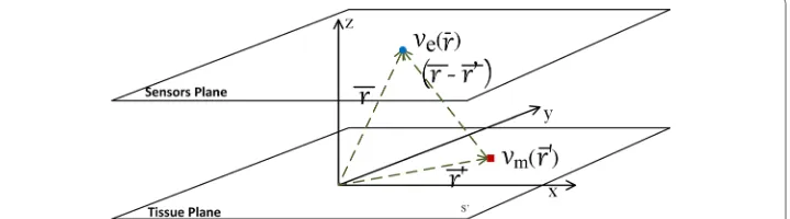
In summary, this mathematical model reformulates the volume conductor equations as a stereotypical current source, and then, the current source passes trough a filter which represents the effect of distance and impedance between the current sources and the recording electrode. In other words, the way the current source is transformed by the effects of distance and impedance to the voltage recorded at a single electrode is formu-lated as a convolutional operator in space. More specifically, the physical model used in this work (see Fig. 1) comprises the uptake of the extracellular potentials at a very close distance of the cardiac tissue. On the one hand, the circulating blood medium is assumed to have homogeneous conductivity. On the other hand, we take into account the source space given by a set of cells in a surface section of cardiac myocyte cells. Finally, the extracellular potential is measured at a fixed distance from these source cells. With these conditions, we can express the physical model as a spatial convolution inte-gral, hence, the physical model can be considered as a LSIS. This formulation allows us to present a formulation in terms of the DSM framework. A preliminary approach to the proposed physical model was reported in [51].
In the present work, we consider the equations for a two-dimensional tissue as seen in Fig. 1. The lower layer corresponds to the cardiac tissue plane, with dimensions l×m
(cm2 ), and it consists of a set of cardiac cells or elements that generate an intracellular potential vm(r′) , where r′ denotes the position of a differential element in this source tis-sue plane. The upper layer corresponds to the horizontal plane where the catching cath-eters are situated during the electrophysiological study. Here, ve(r) corresponds to the extracellular potential captured by the catheters of all cardiac tissue cells activated in the instant t=t0 at a constant height z=z0 of the tissue, and r represents the general posi-tion of a differential catchment element. Note that height z=z0 represents and can be seen as the radio of the metallic catheter integrating the electrical activity in its surface, in order to avoid undetermination in the mathematical equations when the catchment catheter is in contact with the tissue. Then, extracellular potential ve(r) is given by
where c=a2σi/4σe , a is the cell or element radio, and σi and σe are the intracellular and extracellular conductivities, respectively. Therefore, |r−r′| is the distance from each
point in the cardiac tissue to each point in the sensors plane [52].
(1)
ve(r)=c
s′
∇2vm(r′)
|r−r′| ds ′
In our model, we use a compact form with the following expression,
so that r′=(x′,y′, 0) are the Cartesian coordinates of the cardiac tissue source cells, and r=(x,y,z0) are the Cartesian coordinates of the observation points in the sensor plane.
Then, Eq. (1) can be rewritten as
This equation represents the forward problem for the extracellular potentials as meas-ured by the catchment catheters (see Fig. 1). With this equation, it can be readily shown that the used model satisfies the properties of linearity and spatial invariance, hence it actually represents a LSIS.
The impulse response of this LSIS can be theoretically identified in order to give an alternative model equation in terms of a spatial convolution. We can find impulse response he(r) in Eq. (3) by inputing a Dirac’s delta function in the spatial domain as a transmembrane potential source, i.e., by making vm(r′)=δ(r′) . In this case, the meas-ured extracellular potential is
By using the properties of the delta function, as shown in Appendix, we further obtain a compact expression for this impulse response,
where * denotes here the possibly multidimensional spatial convolution. We have to keep in mind that we are specifically using here he(r)= ∇2Ŵ(r)
r=(x,y,z0) , as detailed in
Appendix. Now, we can propose a forward problem which is stated as a convolutional problem, and the equation can be seen as the definition of a convolutional, spatial, and two-dimensional signal model [53], just given by
This equation is valid throughout the space occupied by the source at z=0 . Without losing the generality, for simplicity, and by working according to the model in Fig. 1, we have:
and we can finally express our fundamental equation as
(2)
Ŵ(r−r′)= c |r−r′| =
c
(x−x′)2+(y−y′)2+z2 0
(3)
ve(r)=
s′(r′)Ŵ(r
−r′)· ∇2v
m(r′)dr′
(4)
he(r)=
s′(r′)Ŵ(r
−r′)· ∇2δ(r′)dr′
(5)
he(r)=
s′(r′)
∇2Ŵ(r−r′)·δ(r′)dr′= ∇2Ŵ(r)∗δ(r)= ∇2Ŵ(r)
(6)
ve(r)=Ŵ(r)∗ ∇2vm(r)=he(r)∗vm(r)
(7)
he(r)= he(r)
z=z0 ve(r)= ve(r)|z=z0
(8)
Equation (6) characterizes the physical model as a LSIS in terms of the convolution operator, hence, we can use the DSM−SVR and benefit from its properties in terms of regularization and generalization capabilities from machine learning. Equation (8) con-tinues to fulfill the convolutional relationship, and we are just accounting for the symme-try in our problem in order to address the two-dimensional signal model. Whereas these equations are general enough to support a three-dimensional model, we will restricts ourselves here to Eq. (8) for the purpose of benchmarking the generalization properties of the DSM−SVR in one- and two-dimensional models, as described later.
Conventional algorithms in the inverse problem in electrophysiology
In order to implement and benchmark the above described equations with commonly used methods for solving the inverse problem, we need to define a discretized form of Eq. (8). For this purpose, a discretized matrix form is first defined, representing the physical model with its corresponding notation. After this, we briefly review the state of the art of the methods used to solve the inverse problem in electrophysiology that are based on this matrix.
To obtain the solution of the forward problem, Eq. (8) can be written into its matrix form as follows,
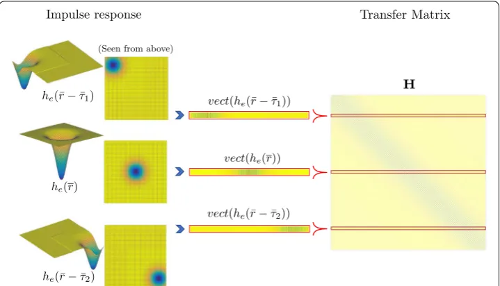
where ve and vm denote the vector form for the transmembrane and for the extracellular potentials, respectively; and H is a Toeplitz symmetric square matrix. The size of this H matrix depends on the number of sensor elements and source elements on the consid-ered planes, and it represents the convolutional matrix of the LSIS. Each of its rows is a vectorized version of a shifted two-dimensional impulse response, he(r) , where Eq. (5)
has been previously discretized in a two-dimensional uniform grid. An example of con-struction of this H matrix is drawn in Fig. 2.
(9)
ve=Hvm,
Fig. 2 Construction scheme of transfer matrix, by using a two‑dimensional uniform impulse response he(r) . Note that vect(he(r−τ )) denotes a vectorization of a two‑dimensional impulse response shifted from the
Now, the inverse problem consists of estimating the transmembrane potential while assuming H and ve known [54–56]. The immediate solution can be expressed as vˆm=H−1ve , where vˆm is the estimated transmembrane potential with this direct matrix inversion. Although transfer matrix H is assumed to be known, usually poor quality results are given by the straightforward inversion, due to the inherent ill-conditioning of the problem matrix. Hence, regularization techniques must be employed in the solution of the inverse problem. One of the most popular solutions of the inverse problem is the Tikhonov regularization [44], which is based on the LS method, and represents a standard approach in estimation analysis to the approxi-mate solution of overdetermined systems. When the optimization objective consists of adjusting the parameters of a model function to its best fit with a data set, the LS method finds its optimum when the sum of squared residuals is minimum. Residuals are defined as the difference between the actual values of the dependent variable and the model predicted values, and in our case are given by
When H matrix in the LS problem is ill-posed, the closed-form solution cannot be applied in a stable way, since small variations in the input data can result in large errors in the solution. A remedy often used in practice is to transform the original problem into one where the ill-posing is compensated for, by adding a term to Eq. (10), and a usual method for stabilizing this inverse solution is to use Tikhonov regularization. In this case, the expression is the following,
and its closed-form solution can be readily shown to be
where γ2 is the regularization penalty parameter, which controls the weight attributed
to constrain condition ||Rvm||2 , and matrix R represents the regularization operator for different orders. For the method of Zero-Order Tikhonov (ZOT) solution [44], operator R is the identity matrix ( Rii=1 ), and thus it is constrained in energy ( l2 norm). Now, if R approximates the first ( Rii = −1 and Rii+1=1 ) or second ( Rii= −1 , Rii+1= 2 and
Rii+2= −1 ) spatial derivatives, then vˆm is known as the First-Order Tikhonov (FOT) [45] or the Second-Order Tikhonov (SOT) [46] solution method, respectively, and it now exhibits a smoother optimization surface gradient or curvature.
Another method used to solve this kind of inverse problems is the TSVD, which solves the following expression:
(10)
ˆ
vm=arg min
vm (||ve−Hvm|| 2)
(11)
ˆ
vm=arg min
vm (||
ve−Hvm||2+γ||Rvm||2)
(12)
ˆ
vm=(HTH+γ2RTR)−1HTve
(13)
ˆ
vm=arg min
where Hk is the reconstruction of H matrix using the k largest singular values. Because this method is based on a Singular Value Decomposition (SVD) process, the regulariza-tion term is defined by the number of used singular values (k), which is known as trun-cation parameter. Note that the order of R matrix also yields different solutions, such as Zero-order Tikhonov SVD (ZTSVD), First-order Tikhonov SVD (FTSVD), or Second-order Tikhonov SVD (STSVD) [47].
Another regularization method is Total Variation (TV), which is similar to Tik-honov technique, but it uses a non-quadratic norm in the regularization term, in par-ticular, often the ℓ1 norm. Hence, the TV solution is obtained by solving the following problem,
where R can be also the Gradient or Laplacian operators, hence obtaining the First-order TV (FTV) [48] and the Second-order TV (STV) [49] solutions, respectively.
All these methods require an accurate determination of the regularization param-eter, whose value determines the intensity and influence of the applied constraints. However, the robustness, quality, and resolution of the inverse solution are not always guaranteed because of the matrix inversion. Therefore, an alternative method is next proposed to solve the inverse problem and formulated in the simple scenarios used in this work.
Equations for the DSM−SVR solution
The SVM are supervised learning models that are widely used to solve machine learn-ing problems [34]. The ν-SVM [57] is a well-known class of SVM algorithm used both for regression and classification. The ν-SVR has been proposed for tuning insensi-tivity parameter ǫ in terms of a new free parameter ν with bounded range in (0, 1) [58], which makes the training process simpler. An additional class of non-linear SVR algorithms for solving convolutional data models can be obtained by considering the non-linear regression of the time instants of the observed signals, and then appro-priately choosing a Mercer’s kernel. This class of algorithms is known as DSM−SVR framework [38], and in this section we present the equations used for this approach and proposed to solve the inverse problem in electrophysiology, according to the con-volutional and multidimensional signal model previously developed in the preceding sections.
Be {[(xi,yi, 0),ve(xi,yi,z0)],i=1,. . .,N} , such that (xi,yi, 0)∈R3 is the position vec-tor in the cardiac tissue plane of the ith source element, and vee(r)=ve(xi,yi,z0) with
z0>0 , are the extracellular potential measurements of the sensor plane. The DSM− SVR uses a primal signal model that represents a regression of the independent vari-able in an unknown space, this is
(14)
ˆ
vm=arg min
vm (||ve−Hvm|| +γ||Rvm||1)
(15)
where φ is a non-linear mapping from the input space to a (usually unknown) Reproduc-ing kernel Hilbert Space (RKHS) [36, 59], and w and b are the linear regressor and bias, respectively. Then, the formulation of the primal problem of DSM−SVR is to minimize
subject to
where ξi(∗) denotes both ξi and ξi∗ slack variables, C is the regularization parameter, and
ν is an approximate ratio of the number of support vectors with respect to the number of training examples. Parameter b can be computed by taking into account that Eqs. (17) become equalities with ξi(∗)=0 for points with 0< αi(∗)<C/N in the Karush–Khun– Tucker (KKT) conditions. In order to obtain the estimated extracellular potential, we solve the optimization problem as described in [34, 38, 39], and the solution takes the form
where κ(r′
i,r′j)= �φ (r′i),φ (r′j)� is a Mercer’s kernel function, and αi(∗) are the Lagrange multipliers [37].
In our formulation, the kernel can be advantageously defined by using h(r) according
to the impulse response of the physical model in Eq. (5), which is compatible with the quasielectrostatic conditions of the cardiac tissue and while mathematically satisfying the Mercer’s condition. It is immediate to see that the following definition fulfills both, thanks to the symmetry properties of the LSIS impulse response,
On the other hand, Lagrange multipliers αi(∗) can be assigned to correspond to the esti-mated intracellular potential, simply as follows,
Now, the solution to the physical model in terms of the DSM−SVR algorithm can be expressed as
As seen, the last equation again corresponds to the convolutional form of a LSIS [60]. Therefore, by fulfilling Eqs. (19) and (20), and thanks to the symmetry of matrix he(r) ,
(16)
1 2 �w�
2+C
νε+ 1
N
N
i=1
(ξi+ξi∗)
(17)
�w,φ ([xi,yi, 0]� +b−ve(xi,yi,z0)≤ǫ+ξi
ve(xi,yi,z0)− �w,φ ([xi,yi, 0]� +b≤ǫ+ξi∗ ξi(∗)≥0, ∀i ǫ≥0
(18)
ˆ
ve(x,y,z0)=
N
i=1
(αi−α∗i)κ([xi,yi, 0],[xj,yj, 0])+b
(19)
κ([xi,yi, 0],[xj,yj, 0])=he(||r′
i−r′j||1)
(20)
(αi−α∗i)= ˆvm(r′i)
(21)
ˆ
ve(r)= N
i=1 ˆ
this DSM−SVR solution has been made to correspond with the same convolutional model in Eq. (8).
Simulations and experiment design
Our tests were performed in one- and two-dimensional tissue models generated with Matlab® by discretization of the continuous space model equations in "Physical model" section. For the one-dimensional case, a tissue line of elements was considered, with source elements aligned with the x-axis, and catchment sensors also aligned and at con-stant height z0 (see Fig. 3). The lengths of the one-dimension cardiac-tissue line and of the catchment-sensor line were the same, hence yielding the same number of source and catchment elements after discretization, see Fig. 3. Simulations were performed with a cardiac tissue length of L=3 cm. The number of cells per millimeter was N =80 cell/ cm, and we had 240 sensor elements at height z0 cm. The intracellular potential was cen-tered at the tissue origin, with depolarization starting at about − 0.5 cm and repolariza-tion ending about 0.5 cm (see e.g. Fig. 8), which ensured that the recorded EGM included the complete depolarization and repolarization phases (spatial support was between
− 1.5 cm and 1.5 cm). Note that, according to this, we did not considered source or sink
EGMs, corresponding to anatomical or functional origin or end of the tissue potential propagation. The one-dimensional model of this cardiac-tissue line was the same as the one used in [51], and further details of this model can be found therein.
For the two-dimensional case, a plane tissue (see again Fig. 1) was considered with catchment sensors at coordinates (x, y) and at constant height z0 . We used a cardiac tis-sue plane with coordinates (x′,y′) and catchment plane at height z0 of the cardiac tissue. Similar to the one-dimensional case, the number of sensor elements was equal to the number of source elements, again see Fig. 1. A 3-cm2 patch of cardiac tissue was sym-metrically situated with respect to the coordinate origin, with 80-elements/cm2 density. Accordingly, the number of sensor elements was 57, 600, all of them situated at z0=0.02 cm height, but computational complexity was controlled by decimating by 2 in both spa-tial dimensions. This extremely high density of sensors aimed to give good quality visu-alization for the results of our experiments. We again considered the transmembrane potential in the center of the cardiac tissue plane to reduce boundary effects.
It can be seen from this experimental setup that the assumptions of constant z0 and plane tissue and sensors are used for fundamental analysis purposes, however, a sensor
array will be in general curve-shaped and with different heights for each sensor. Whereas this has clear implications on the clinical use, this spatial distortion due to non-constant height and curvature was not considered here, but rather we focused on the fundamen-tals of the more basic problem of plane tissue and sensors.
We benchmarked the DSM−SVR algorithm introduced in Section with several of the most traditionally used methods among those ones explained in Section. Specifically, we chose FTSVD, FOT, and FTV algorithms, and in order to optimize the regulariza-tion parameter we tested the use of two different strategies, namely, the L-Curve and the Leave-One-Out (LOO) methods. The L-Curve is supported by a graphical representa-tion for a set of valid regularizarepresenta-tion parameters of the (semi)norm of the normalized solution versus the corresponding norm of the residuals in Eq. (11). An essential feature of the L-Curve is that the optimal regularization parameter is not far from the regulari-zation parameter that corresponds to this L-Curve corner [61]. In the LOO method, the complete data set except one sample is used to build the model, and the out-of-sample observation is used to calculate its estimation error, so that by repeating the procedure for all the samples and averaging, the generalization error is obtained for each value of the free parameter. A similar strategy was followed for the free-parameter search of DSM−SVR, and also the L-Curve was adjusted by using LOO methods according to the Mean Absolute Error (MAE), both of them in terms of signal-to-noise ratio (SNR), when the noise was introduced in the observations, and in terms of the transfer-matrix-to-noise ratio (so-called here HNR).
Results
In this section, we present the results obtained with the proposed DSM−SVR approach
when solving the intracardiac inverse problem. A preliminary study is presented show-ing the ill-conditionshow-ing character of the problem with the used model and different estimation algorithms. After this, the first study was addressed in the one-dimensional model in order to determine the catchment height yielding a realistic waveform for the intracardiac EGM. Then, the following experiments were performed, both for the one- and two-dimensional models: (a) a method was scrutinized for determining the free parameters of the DSM−SVR algorithm; (b) the impact of different noise intensities was analyzed both when present on the EGM and on the transfer matrix; and (c) results were benchmarked with several methods selected among those ones that have been previ-ously used in the inverse problem literature.
Ill‑conditioning analysis
In our problem, the ill-conditioning in the transfer matrix comes from the fact that matrix H is built, and in essence it consists of short-delayed versions of the impulse response, i.e., if the impulse response in a single-dimensional model is given by h(x), the Toeplitz matrix consists of rows which are basically given by h(x−�x) , and for small
tuning their free parameters as later described. As seen in Fig. 4, different artifacts can be seen in the different methods, which mostly consist of a drift or leakage from the baseline and some oscillations close to the impulse activation. In frequency, this can be seen as a strong distortion in the low-frequency components of the estimated transfer function. Note that this transfer function is not just the one given by the forward prob-lem, but also it includes the algorithm sensitivity. Accordingly, those methods which require matrix inversion are more sensitive to this effect, whereas the DSM−SVR with
Laplacian kernel is built with a forward-problem formulation and the use of kernels in the formulation does not require matrix inversion in the estimation process.
Fig. 4 Ill‑conditioning of the inverse problem in electrophysiology. A delta function is used as a source, and it is estimated in space (down) by different methods and for different SNR. The corresponding frequency responses are calculated (up): a SNR=15 dB; b SNR=25dB; c SNR=35 dB. Note that H(ω) denotes the
frequency response after tuning the free parameters on each method, and h(x) denotes the impulse
Determination of a suitable catchment height
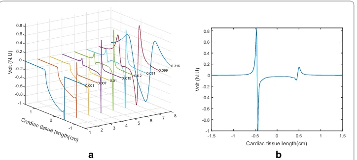
Height tests were run on the sensor plane to determine the optimal height at which the signal of the extracellular potential in the one-dimensional tissue had a wave-form similar to the unipolar EGMs that are usually seen in the clinical practice as a function of time in a catching electrode at a fixed position. The range of heights for z0 in which the plane of sensors was varied with respect to the plane of the car-diac tissue was between 0.001 and 0.4 cm, and very different EGM waveforms were obtained throughout this range, as seen in Fig. 5a. Note that for extremely close z0 , the Laplacian discretization is distorted into near an inverted delta function, whereas for extremely large z0 the EGM turns a far-field waveform. For intermediate values of
z0 , there are different and intermediate distortion effects. We can check that z0=0.02 cm in panel (b) was similar enough to the usual unipolar EGM waveform seen in elec-trophysiological studies. Accordingly, this was the catchment height used for all the subsequent studies, both in the one- and in the two-dimensional models.
Free‑parameter tuning strategy
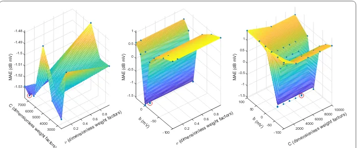
The DSM−SVR algorithm needs to previously determine a set of free parameters, which are ν , γ , C, and b. Given that these parameters are often strongly interdependent, some-times this can represent a complex search procedure if we wanted to follow a regular grid strategy, as far as all-combined-with-all evaluation would give a extremely high amount of parameter combinations to be evaluated. Instead, we followed a non-uniform grid strategy for tuning the free parameters, as follows: (a) a lower and an upper limit were established for the possible rank of each of these four free parameters; (b) accord-ing to a previous run of searched parameters, each of them was established on either a linear or a logarithmic rank scale; (c) for each range, a middle point was established in each free parameter; (d) for all the combinations of the three values on each free param-eter, a machine was trained using all the model observations except one, then the valida-tion error was obtained for the out-of-sample observavalida-tion, the process was repeated for all the observations, and out-of-sample errors were averaged; (e) the minimum error was used to reduce the range interval in the free parameters; (f) steps from (c) to (e) were
-1 -0.8 -0.6 -0.4 -0.2 0 1 Volt (N.U ) 0.2 0.4 0.6 8 0.8 7 Cardiac tissue length(cm ) 0 0.316 6 0.099 5 0.031 4 0.02 3 -1 0.015 2 0.01 1 0.007 0.001
-1.5 -1 -0.5 0 0.5 1 1.5 Cardiac tissue length(cm)
-1 -0.8 -0.6 -0.4 -0.2 0 0.2 0.4 0.6 0.8 Volt (N.U ) b a
Fig. 5 Unipolar EGM waveforms obtained with different values of z0 , normalized to its maximum amplitude
repeated according to the new set of points in the grid. This procedure showed to con-verge in the set of observed cases. Figure 6 depicts some slice examples of the surfaces that were obtained and built with this strategy. We can see that, in general, regions with good performance correspond either to clear minimum or to flat zones, which supports the search for further specific methods to substantially reduce the computational burden associated to the free parameter search.
Noise conditions and benchmarking
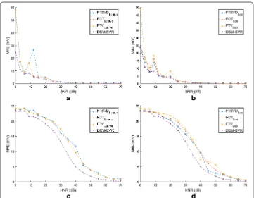
The robustness of the different algorithms was benchmarked in terms of the MAE on the two-dimensional domain. Given that we used a simulation model, we had available the actual solution of the transmembrane potential in the surface source. We added white-Gaussian noise with different power to the model in two ways. On the one hand, noise was added to the observations, i.e., to the observed extracellu-lar potentials, as far as this is the kind of robustness more widely scrutinized in the inverse problem literature. On the other hand, noise was added to the transfer matrix, accounting for keeping its symmetry properties intact when doing so. This kind of test is less usual in the literature, however, we wanted to check for the sensitivity of the methods to the possible presence of errors in the transfer matrix errors in those scenarios when the transfer matrix is not so well-known in advance. For each method, we obtained the MAE as a function of the SNR and of the HNR. In both cases, we evaluated the performance for SNR between 0 and 70 dB.
Figure 7 shows the results obtained for all the used methods with SNR and HNR. On the one hand, panels (a, b) correspond to the SNR case with L-Curve and LOO, respectively. We can see that the MAE consistently decreases with increasing SNR in the catchment sensors. Also, the MAE is high for values of SNR below 5 dB, whereas it comes negligible after 30 dB. This behavior is in general consistent for all the meth-ods, however, the DSM−SVR algorithms has a noticeably lower MAE in low-SNR conditions, and a consistently yet slightly lower MAE in high-SNR conditions. We can also see that the LOO approach tends to provide noisier MAE curves for intermediate
-1.53
7000 -1.52 -1.51
6000
MAE (dB mV
) -1.5 0.8 C (d imensi onles s we ight fact ors) -1.49 5000 0.6 (dimensi onless weight factors) -1.48 4000 0.4 0.2 3000 -1.5 -1 -0.5 0
MAE (dB mV
) 0 0.8 b (m V) 0.5 0.6 (dimensionless weight fact ors) 1 -50 0.4 0.2 -100 -1.5 100 -1 -0.5 50 10000 0
MAE (dB mV
)0.5
8000
b (mV)0 1 6000 C (dime nsionless weight factors) 4000 -50 2000 -100
SNR conditions in most of the classic algorithms, though it does not affect the DSM−
SVR algorithm free-parameter search.
On the other hand, panels (c, d) in Fig. 7 show a different behavior of MAE as a function of HNR. First, the shape of the MAE variation is dome-like here, whereas it was exponential-like for the MAE in terms of SNR. Second, it remains at a more moderate level for low HNR values, when compared with the same range in the SNR, starting in general between 23 and 25 mV of MAE. And third, this dome-like vari-ation is in general (and except for the range below 5 dB) above the MAE in terms of SNR. This means that these algorithms are clearly more sensitive to noise in the transfer matrix than to noise in the observations. Moreover, in the HNR plots we can see that there is a noticeable advantage of the DSM−SVR algorithm in comparison with the classical algorithms, indicating that this method is more robust when faced to perturbations in the transfer function estimation. We can finally also see also that slightly less smooth curves are obtained for the HNR in the classical methods with LOO strategy for the free parameters.
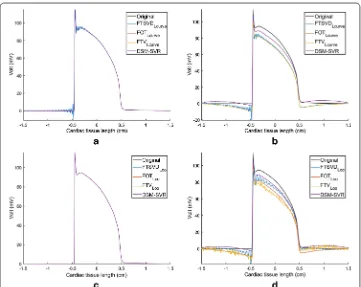
Figure 8 shows the estimated potentials in the line of source elements for the classical and for the DSM−SVR methods. Panels (a, c) show that the free-parameter estimation in the trivial case of no-noise present is clearly addressed by all the methods, though FTSVD exhibits ringing in the boundary of extremely fast variations, i.e., before and after the depolarization phase (but not in smooth variations as the repolarization phase). Pan-els (b, d) show the estimated transmembrane potentials for an example of intermediately
high HNR of 45 dB. Overall, all the methods tend to deviate from flat regions in the presence of either sharp or smooth boundaries (depolarization or repolarization phases, respectively). Whereas DSM−SVR also exhibits this behavior, nevertheless it remains closer to the actual spatial waveform. In these conditions, LOO free-parameter search tends to give ringing solutions in the classical algorithms, whereas this is not the case for L-Curve search, though FTSVD still exhibits some ringing therein.
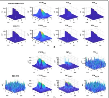
Two‑dimensional simulations
Figures 9 and 10 depict some examples of the estimation behavior with the tested meth-ods. Panel (a) shows the ideal and the estimated transmembrane potentials as a function of the two-dimensional spatial coordinates. In order to better understand the quality of the simulations, panel (b) depicts the absolute residuals as a function of the same spatial coordinates. It can be seen therein that the DSM−SVR provides a uniform distribution of the residuals with space, in contrast with FTSVD (either with LOO or with L-Curve) and with FOT (with LOO), which exhibit strong boundary effects and locally aberrant increment of the residuals. On the other hand, FOT with L-Curve yields a heteroske-dastic residual distribution, which tends to increase at the inside and to reduce at the boundaries. Finally, FTV with L-Curve shows similar results to DSM−SVR, and
some-times even slightly better results when using LOO for its free-parameter tuning. Note that FTV is not the most widely used method in the current literature of the inverse
problem in electrophysiology, and that its behavior with LOO free-parameter search had not been previously addressed.
Table 1 shows the MAE results for all the used methods with HNR and SNR cases using L-Curve and LOO in the traditional algorithms, and for grid search in the DSM−
SVR algorithm. As can be seen, the MAE is now more similar in SNR compared with HNR, with a trend on MAE to be larger on SNR for similar noise ratios, probably due to the much larger number of observations in the two-dimensional discretized model. For the LOO tuning, the MAE tends to be smaller than for L-Curve tuning, but computa-tional cost in the L-Curve free-parameter tuning is much smaller. On the other hand, the MAE in HNR is similar between FTV with L-Curve and DSM−SVR, the last one being slightly better in the cases with noise. The MAE in SNR exhibits similar values for FTV with L-Curve and DSM−SVR, the last one being slightly better with SNR greater than 40 dB. In the case of the LOO, the types of noise produce different MAE among meth-ods, with the best performance reached in general by the FTV algorithm. Note that both FOT and DSM−SVR are significantly better than the other classical methods in the two-dimensional scenarios, and that the DSM−SVR algorithm is again slightly better than the FTV with L-Curve, but not so much margin can be seen now between DSM−SVR and FTV methods.
Discussion
In recent years, research on the inverse problem in electrophysiology has been in con-stant development, but it is still open to improvements in its algorithms in terms of
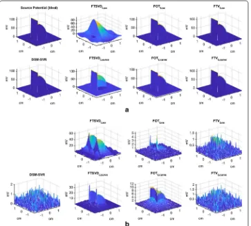
Fig. 10 Details on the simulation results in the two‑dimensional model, for HNR = 40 db. a Transmembrane potentials as a function of spatial coordinates, for the ideal and the estimated versions. b Absolute residuals for the estimated transmembrane potentials in (a)
Table 1 Results on noise robustness of the methods in the two-dimensional model
MAE has been calculated for all the tested methods as a function of SNR and of HNR, and also when using L‑Curve versus the LOO with traditional algorithm for the free‑parameter search and Grid search for DSM−SVR
HNR MAE (mV) SNR MAE (mV)
L‑Curve
(dB) 25 30 40 50 ∞ 25 30 40 50 ∞
FTSVD 1.768 1.862 1.269 0.145 1.051 2.266 1.507 8.044 0.192 1.051 FOT 3.094 2.433 1.791 1.599 1.517 4.230 2.734 1.703 1.530 1.518 FTV 1.766 1.066 0.366 0.117 8.11e−12 4.032 2.233 0.697 0.226
8.11e−12 LOO
FTSVD 7.846 7.97 8.015 8.026 8.011 8.030 8.017 8.013 8.011 8.011 FOT 1.363 0.867 0.335 0.116 4.58e−13 1.188 0.900 0.499 0.210
4.58e−13
FTV 1.388 0.805 0.258 0.083 7.88e−12 2.112 1.197 0.380 0.117 7.88e−12
Grid search
DSM−SVR 1.754 1.053 0.354 0.107 3.28e−4 4.030 2.232 0.696 0.225
resolution and regularization. In this work, we addressed the formulation of the inverse problem using a well-known technique in the machine learning literature, specifically, the SVR following the DSM principles. This methodology had been previously used for creating digital signal processing algorithms from time-convolutional signal mod-els. In our approach, the signal model is tackled by including in the equations (through the Mercer’s kernel and the Lagrange multipliers) the quasielectrostatic field equation conditions as a priori knowledge of the problem. We tested this approach in detailed simulations with synthetic experiments, using one- and two-dimensional models. Benchmarking was made with selected algorithms from classical and recent literature.
Our results showed that the inverse problem in electrophysiology is more sensitive to noise in the estimation of the transfer matrix than in the noise of the observed extracel-lular signals. The DSM−SVR in one-dimensional scenarios exhibited remarkable advan-tage with respect to all the benchmarked algorithms, specially in terms of HNR, whereas in two-dimensional scenarios it was significantly better than classical algorithms, but similar to FTV algorithms. Further research needs to be devoted to scrutinize the best (probably combined) way to tackle with high-dimensional domains. However, robust-ness with respect to the transfer matrix estimation seems to be a key property, which has received little attention in the literature. This advantage, mostly visible in one-dimen-sional simulations, probably comes from the fact that DSM−SVR does not require any kind of inversion, but its formulation rather consists of a direct problem solving and the Structural Risk Minimization Principle. In addition, it has been observed in our results that the depolarization phase is sometimes better fitted than the repolarization phase in the presence of noise. The good behavior of the algorithm in depolarization phase is likely due to its non-inversion nature, which avoids the low-pass effect implicitly asso-ciated to many regularization methods that work with matrix inversions, whereas the repolarization error could be attributed to some deviation in the free parameter search. Nevertheless, further theoretical results should be established in this setting, for pro-viding a more solid framework when working in more complex scenarios. On the other hand, we have seen that the free-parameter tuning in the DSM−SVR can be further optimized, using techniques that require less computational cost.
in the tissue and in the sensors. From a clinical point of view, the number of sensing electrodes needs to be reasonable, as far as they will be placed on (or in) the patient on a comfortable, stable, and easy to put-and-remove way.
On the other hand, our current formulation consists on a mathematical forward model providing with the potential measured in a spatial point by a point-electrode. It is very likely that the inclusion of the shape and volume of the electrode (spherical, ring, oth-ers) can be readily included in the model, which has not yet been addressed in this work. Moreover, it is possible to think on using the method for the estimation of the trans-membrane potentials for larger distances and for non-contact mapping schemes. We performed additional simulations (not included here) showing that for small changes in distance, the impulse response exhibits little (still noticeable) variation on its width, but the methods still work properly. If longer distance are scrutinized, the impulse response gets still wider, and the EGM morphology is noticeably affected. In any case, this in-silico model is not accounting for curvature effects, which could be present. Ideally, a method for estimating the impulse response would strongly improve and extend the scope of the method, which can be incorporated to the proposed method, but it has not been addressed in this work. We focused here on simple propagation, nevertheless, our view is that in fibrillatory rhythms the accurate estimation of the underlying transmem-brane potentials should be strongly informative, as far as their mechanisms still remains unknown. A great amount of knowledge on fibrillatory rhythms has been established by detailed computer simulations on transmembrane potentials and ionic currents [62–64]. However, it is desirable to improve the method in more electrophysiologically simple situations before moving to complex mechanisms.
Conclusion
The proposed approach to the DSM−SVR algorithm with Laplacean kernel can be an effective alternative in the inverse problem in electrophysiology. Our proposed DSM−
SVR algorithm with Laplacian distance kernel can be an efficient alternative to improve the resolution in current and emerging intracardiac imaging systems. The sensitivity of traditional methods to noise in the transfer matrix estimation also needs to be generally taken into account by algorithms in this field.
Authors’ contributions
RCC studied the elaboration of the algorithms, on the mathematical development of the equations, and theprogram‑ ming of the first version of the code. SMR programmed the validation algorithms and worked on codeoptimization and algorithms. MSJ helped in the development of the problem and in the development of thealgorithms. AGA assisted in the clinical part of the investigation. JLRA presented the first development of equations,helping to improve the algo‑ rithms and supervision of the study. All authors read and approved the final manuscript.
Author details
1 Department of Signal Theory and Communications and Telematics and Computation, Rey Juan Carlos University,
Camino del Molino s/n, 28943 Fuenlabrada, Madrid, Spain. 2 Center for Computational Simulation, Universidad Politéc‑
nica de Madrid, Madrid, Spain. 3 Arrhythmia Unit, Hospital General Universitario Virgen de la Arrixaca, El Palmar, Murcia,
Spain.
Competing interests
The authors declare that the research was conducted in the absence of any commercial or financial relationshipsthat could be construed as a potential competing interests.
Funding
Appendix: Model equations
We include here the development of Eq. 5 that has been used for the demonstration of the quasielescastostatic model in see Fig. 1 corresponding to a LSIS. For this purpose, we use the properties of the one-dimensional Dirac’s delta function that can be found in [53, 65] and readily generalized to a two-dimensional domain. Equation 2 can be represented by its Cartesian coordinates as r=(x,y,z0) and r′=(x′,y′, 0) , and then, it can be rewrit-ten as
where x(′) denote both (x,x′) and of the same form can y(′) denote (y,y′) , and similarly
ve(r) and vm(r′) in Cartesian coordinates can be rewritten in our case as
Now, if we replace these expressions in Eq. 3, the cardiac model can be expressed in Car-tesian coordinates, as
With this equation, we can prove that the cardiac model of Fig. 10 represents an LSIS. By replacing vm(x′,y′)=δ(x′,y′) , we have that the impulse response can be expressed as
To solve this equation, we apply the properties of Dirac’s delta function [53, 65], which allows us to obtain
(22)
Ŵ(r−r′)=Ŵ(x(′)
,y(′),z0)
vm(r′)=vm(x′,y′, 0)=vm(x′,y′)
ve(r)=ve(x,y,z0)
ve(x,y,z0)=
s(x′,y′)
Ŵ(x(′),y(′),z0)∇2vm(x′,y′)dx′dy′
he(x,y,z0) =
s(x′,y′)
Ŵ(x(′),y(′),z0)∇2δ(x′,y′)dx′dy′
=
s(x′,y′)
Ŵ(x(′),y(′),z0)
∂2δ(x′,y′) ∂x′2 +
∂2δ(x′,y′) ∂y′2
dx′dy′
=
s(x′,y′)
Ŵ(x(′),y(′),z0)
∂2δ(x′,y′) ∂x′2 +Ŵ(x
(′)
,y(′),z0)
∂2δ(x′,y′) ∂y′2
dx′dy′
he(x,y,z0) =
s(x′,y′)
∂2Ŵ(x(′),y(′),z0) ∂x′2 δ(x
′
,y′)+ ∂
2Ŵ(x(′),y(′),z 0) ∂y′2 δ(x
′
,y′)
dx′dy′
=
s(x′,y′)δ(x ′
,y′)
∂2Ŵ(x(′),y(′),z0) ∂x′2 +
∂2Ŵ(x(′),y(′),z0) ∂y′2
dx′dy′
=
s(x′,y′)δ(x
′,y′)∇2Ŵ(x(′),y(′),z 0)dx′dy′
=
s(r′)δ(r
And finally, we have to keep in mind that
This expression allows us to obtain Eq. (5), which represents the impulse response, and allows us to represent our problem as a two-dimensional convolutional problem.
Publisher’s Note
Springer Nature remains neutral with regard to jurisdictional claims in published maps and institutional affiliations.
Received: 17 March 2018 Accepted: 13 June 2018
References
1. Josephson ME. Josephson clinical cardiac electrophysiology. Alphen aan den Rijn: Wolters Kluwer; 2018. 2. Lou C, Li R, Li Z, Liang T, Wei Z, Run M, Yan X, Liu X. Flexible graphene electrodes for prolonged dynamic ecg moni‑
toring. Sensors. 2016;16(11):1833.
3. Gradl S, Cibis T, Lauber J, Richer R, Rybalko R, Pfeiffer N, Leutheuser H, Wirth M, von Tscharner V, Eskofier BM. Wear‑ able current‑based ecg monitoring system with non‑insulated electrodes for underwater application. Appl Sci. 2017;7(12):1277.
4. Peng Y, Wang X, Guo L, Wang Y, Deng Q. An efficient network coding‑based fault‑tolerant mechanism in wban for smart healthcare monitoring systems. Appl Sci. 2017;7(8):817.
5. Sahoo PK, Thakkar HK, Lin W‑Y, Chang P‑C, Lee M‑Y. On the design of an efficient cardiac health monitoring system through combined analysis of ecg and scg signals. Sensors. 2018;18(2):379.
6. Zhang N, Zhang J, Li H, Mumini OO, Samuel OW, Ivanov K, Wang L. A novel technique for fetal ecg extraction using single‑channel abdominal recording. Sensors. 2017;17(3):457.
7. Everss‑Villalba E, Melgarejo‑Meseguer FM, Blanco‑Velasco M, Gimeno‑Blanes FJ, Sala‑Pla S, Rojo‑Álvarez JL, García‑Alberola A. Noise maps for quantitative and clinical severity towards long‑term ecg monitoring. Sensors. 2017;17(11):2448.
8. Jiang Y, Samuel OW, Liu X, Wang X, Idowu PO, Li P, Chen F, Zhu M, Geng Y, Wu F, et al. Effective biopotential signal acquisition: comparison of different shielded drive technologies. Appl Sci. 2018;8(2):276.
9. Li H, Yuan D, Wang Y, Cui D, Cao L. Arrhythmia classification based on multi‑domain feature extraction for an ecg recognition system. Sensors. 2016;16(10):1744.
10. Raka AG, Naik GR, Chai R. Computational algorithms underlying the time‑based detection of sudden cardiac arrest via electrocardiographic markers. Appl Sci. 2017;7(9):954.
11. Jung W‑H, Lee S‑G. Ecg identification based on non‑fiducial feature extraction using window removal method. Appl Sci. 2017;7(11):1205.
12. Torrecilla EG. Navigation systems in current electrophysiology. Revista Española de Cardiología. 2004;57(08):722–4. 13. Chen Z, Cabrera‑Lozoya R, Relan J, Sohal M, Shetty A, Karim R, Delingette H, Gill J, Rhode K, Ayache N, Taggart P,
Rinaldi C, Sermesant M, Razavi R. Biophysical modeling predicts ventricular tachycardia inducibility and circuit morphology: A combined clinical validation and computer modeling approach. J Cardiovasc Electrophysiol. 2016;27(7):851–60.
14. Paul T, Windhagen‑Mahnert B, Kriebel T, Bertram H, Kaulitz R, Korte T, Niehaus M, Tebbenjohanns J. Atrial reentrant tachycardia after surgery for congenital heart disease: endocardial mapping and radiofrequency catheter ablation using a novel, noncontact mapping system. Circulation. 2001;103(18):2266–71.
15. Rudy Y, Oster HS. The electrocardiographic inverse problem. Crit Rev Biomed Eng. 1992;20(1–2):25–45. 16. Rudy Y. Noninvasive electrocardiographic imaging of arrhythmogenic substrates in humans. Circ Res.
2013;112(5):863–74.
17. Andrews CM, Srinivasan NT, Rosmini S, Bulluck H, Orini M, Jenkins S, Pantazis A, McKenna WJ, Moon J, Lambiase PD, Rudy Y. Electrical and structural substrate of arrhythmogenic right ventricular cardiomyopathy determined using noninvasive electrocardiographic imaging and late gadolinium magnetic resonance imaging. Circ Arrhythmia Electrophysiol. 2017;10(7).
18. Cuculich P, Schill M, Kashani R, Mutic S, Lang A, Cooper D, Faddis M, Gleva M, Noheria A, Smith T, Hallahan D, Rudy Y, Robinson C. Noninvasive cardiac radiation for ablation of ventricular tachycardia. N Engl J Med. 2017;377(24):2325–36.
19. Schilling R, Kadish A, Peters N, Goldberger J, Davies DW. Endocardial mapping of atrial fibrillation in the human right atrium using a non‑contact catheter. Eur Heart J. 2000;21(7):550–64.
20. Schilling RJ, Peters NS, Davies DW. Simultaneous endocardial mapping in the human left ventricle using a noncontact catheter: comparison of contact and reconstructed electrograms during sinus rhythm. Circulation. 1998;98(9):887–98.
21. Yamaguchi T, Tsuchiya T, Miyamoto K, Nagamoto Y, Takahashi N. Characterization of non‑pulmonary vein foci with an ensite array in patients with paroxysmal atrial fibrillation. Europace. 2010;12(12):1698–706.
(23)
he(r) = ∇2Ŵ(r)
22. Nair M, Yaduvanshi A, Kataria V, Kumar M. Radiofrequency catheter ablation of ventricular tachycardia in arrhythmo‑ genic right ventricular dysplasia/cardiomyopathy using non‑contact electroanatomical mapping: single‑center experience with follow‑up up to median of 30 months. J Interv Cardiac Electrophysiol. 2011;31(2):141–7. 23. Bakushinsky A, Goncharsky A. Ill‑posed problems: theory and applications. Berlin: Springer; 1994. 24. Tikhonov AN. Numerical methods for the solution of ill‑posed problems, vol. 328. Berlin: Springer; 1995. 25. Austen G, Grafarend E, Reubelt T. Analysis of the earth’s gravitational field from semi‑continuous ephemeris of a
low earth orbiting GPS‑tracked satellite of type CHAMP, GRACE or GOCE. In: Adam J, Schwarz KP, editors. Vistas for Geodesy in the New Millennium. Berlin: Springer; 2002. p. 309–15.
26. Phillips C, Rugg MD, Friston KJ. Systematic regularization of linear inverse solutions of the EEG source localization problem. NeuroImage. 2002;17(1):287–301.
27. Beretta E, Manzoni A, Ratti L. A reconstruction algorithm based on topological gradient for an inverse problem related to a semilinear elliptic boundary value problem. Inverse Probl. 2017;33(3):035010.
28. Ramanathan C, Jia P, Ghanem R, Calvetti D, Rudy Y. Noninvasive electrocardiographic imaging (ECGI): application of the generalized minimal residual (GMRes) method. Ann Biomed Eng. 2003;31(8):981–94.
29. Rodrigo M, Climent A, Liberos A, Hernandez‑Romero I, Arenal A, Bermejo J, Fernandez‑Aviles F, Atienza F, Guillem M. Solving inaccuracies in anatomical models for electrocardiographic inverse problem resolution by maximizing reconstruction quality. IEEE Trans Med Imaging. 2018;37(3):733–40.
30. Onak ON, Dogrusoz YS, Weber GW. Effects of a priori parameter selection in minimum relative entropy method on inverse electrocardiography problem. Inverse Probl Sci Eng. 2018;26(6):877–97.
31. Bai MR, Chung C, Wu P‑C, Chiang Y‑H, Yang C‑M. Solution strategies for linear inverse problems in spatial audio signal processing. Appl Sci. 2017;7(6):582.
32. Serinagaoglu Y, Brooks DH, MacLeod RS. Improved performance of bayesian solutions for inverse electrocardiogra‑ phy using multiple information sources. IEEE Trans Biomed Eng. 2006;53(10):2024–34.
33. Yao B, Zhu R, Yang H. Characterizing the location and extent of myocardial infarctions with inverse ecg modeling and spatiotemporal regularization. IEEE J Biomed Health Inform. 2017.
34. Vapnik V. The nature of statistical learning theory. Berlin: Springer; 2013.
35. Jiang M, Zhu L, Wang Y, Xia L, Shou G, Liu F, Crozier S. Application of kernel principal component analysis and sup‑ port vector regression for reconstruction of cardiac transmembrane potentials. Phys Med Biol. 2011;56(6):1727. 36. Cristianini N, Shawe‑Taylor J. An introduction to support vector machines and other Kernel‑based learning methods.
Cambridge: Cambridge University; 2000.
37. Camps‑Valls G, Rojo‑Álvarez JL, Martínez‑Ramón M. Kernel methods in bioengineering, signal and image process‑ ing. Hershey: Igi Global; 2006.
38. Rojo‑Álvarez JL, Martínez‑Ramón M, Muñoz‑Marí J, Camps‑Valls G. A unified SVM framework for signal estimation. Digital Signal Process. 2014;26:1–20.
39. Rojo‑Álvarez JL, Martínez‑Ramón M, Muñoz‑Marí J, Camps‑Valls G, Cruz CM, Figueiras‑Vidal AR. Sparse deconvolu‑ tion using support vector machines. EURASIP J Adv Sig Process. 2008;2008(1).
40. Rojo‑Álvarez JL, Martínez‑Ramón M, Muñoz‑Marí J, Camps‑Valls G. Digital signal processing with Kernel methods. Hoboken: Wiley; 2018.
41. Saiz J, Gomis‑Tena J, Monserrat M, Ferrero JM, Cardona K, Chorro J. Effects of the antiarrhythmic drug dofetilide on transmural dispersion of repolarization in ventriculum. A computer modeling study. IEEE Trans Biomed Eng. 2011;58(1):43–53.
42. Dux‑Santoy L, Sebastian R, Felix‑Rodriguez J, Ferrero JM, Saiz J. Interaction of specialized cardiac conduction system with antiarrhythmic drugs: a simulation study. IEEE Trans Biomed Eng. 2011;58(12):3475–8.
43. Martinez‑Mateu L, Romero L, Ferrer‑Albero A, Sebastian R, Matas JFR, Jalife J, Berenfeld O, Saiz J. Factors affect‑ ing basket catheter detection of real and phantom rotors in the atria: A computational study. PLoS Comput Biol. 2018;14(3):1006017.
44. Tikhonov AN, Arsenin VI, John F. Solutions of ill‑posed problems, vol. 14. Washington, DC: Winston; 1977. 45. Franzone PC, Taccardi B, Viganotti C. An approach to inverse calculation of epicardial potentials from body surface
maps1. In: Kornreich F, editor. Electrocardiology III/vectorcardiography, vol. 21. Basel: Karger Publishers; 1978. p. 50–4.
46. Brooks DH, Ahmad GF, MacLeod RS, Maratos GM. Inverse electrocardiography by simultaneous imposition of multi‑ ple constraints. IEEE Trans Biomed Eng. 1999;46(1):3–18.
47. Hansen PC. Rank‑deficient and discrete ill‑posed problems: numerical aspects of linear inversion. Philadelphia: Society for Industrial and Applied Mathematics (SIAM); 1998.
48. Ghosh S, Rudy Y. Application of l1‑norm regularization to epicardial potential solution of the inverse electrocardiog‑ raphy problem. Ann Biomed Eng. 2009;37(5):902–12.
49. Brooks DH, Srinidhi KG, MacLeod RS, Kaeli DR. Multiply constrained cardiac electrical imaging methods. In: SPIE’s international symposium on optical science, engineering, and instrumentation. International Society for Optics and Photonics; 1999. p. 62–71
50. Ellis WS, Eisenberg SJ, Auslander DM, Dae MW, Zakhor A, Lesh MD. Deconvolution: a novel signal processing approach for determining activation time from fractionated electrograms and detecting infarc ted tissue. Circula‑ tion. 1996;94(10):2633–40.
51. Caulier‑Cisterna R, Sanromán‑Junquera M, Rojo‑Álvarez JL, García‑Alberola A. A support vector laplacian distance kernel approach to the inverse problem in intracardiac electrophysiology. In: XIV mediterranean conference on medical and biological engineering and computing. 2016;2016:89–94.
52. Plonsey R, Barr RC. Bioelectricity: a quantitative approach. Berlin: Springer; 2007.
53. Bracewell RN. ch. 5: The impulse symbol. The Fourier transform and its applications. 3rd ed. New York: McGraw‑Hill; 1999. p. 69–97.
• fast, convenient online submission •
thorough peer review by experienced researchers in your field • rapid publication on acceptance
• support for research data, including large and complex data types •
gold Open Access which fosters wider collaboration and increased citations maximum visibility for your research: over 100M website views per year •
At BMC, research is always in progress.
Learn more biomedcentral.com/submissions
Ready to submit your research? Choose BMC and benefit from:
55. Voth EJ. The inverse problem of electrocardiography: industrial solutions and simulations. Int J Bioelectromagn. 2005;7:191–4.
56. Gulrajani RM. The forward and inverse problems of electrocardiography. IEEE Eng Med Biol Mag. 1998;17(5):84–101. 57. Schölkopf B, Smola AJ, Williamson RC, Bartlett PL. New support vector algorithms. Neural Comput.
2000;12(5):1207–45.
58. Chang C‑C, Lin C‑J. Training ν‑support vector regression: theory and algorithms. Neural Comput. 2002;14(8):1959–78.
59. Schölkopf B, Smola AJ. Learning with Kernels: support vector machines, regularization, optimization, and beyond. Cambridge: MIT Press; 2002.
60. Oppenheim AV. Discrete‑time signal processing. New York: Pearson Education; 1999.
61. Hansen PC. The l‑curve and its use in the numerical treatment of inverse problems. In: Jonhston P, editor. Computa‑ tional inverse problem in electrocardiography. Ashurst: WIT Press; 2001.
62. Schalk M, Heinke M, Hörth J. Heart rhythm model and simulation of electrophysiological studies and high‑fre‑ quency ablations. EP Europace. 2017;19(suppl_3):iii183.
63. Rodrigo M, Climent AM, Liberos A, Fernández‑Avilés F, Berenfeld O, Atienza F, Guillem MS. Highest dominant fre‑ quency and rotor positions are robust markers of driver location during noninvasive mapping of atrial fibrillation: a computational study. Heart Rhythm. 2017;14(8):1224–33.