Quantifying the impact of sub-grid surface wind variability on sea salt and dust emissions in CAM5

www.geosci-model-dev.net/9/607/2016/ doi:10.5194/gmd-9-607-2016

© Author(s) 2016. CC Attribution 3.0 License.

Quantifying the impact of sub-grid surface wind variability on sea

salt and dust emissions in CAM5

Kai Zhang1, Chun Zhao1, Hui Wan1, Yun Qian1, Richard C. Easter1, Steven J. Ghan1, Koichi Sakaguchi1, and Xiaohong Liu2

1_{Pacific Northwest National Laboratory, Richland, WA, USA}

2_{Department of Atmospheric Science, University of Wyoming, Laramie, WY, USA} Correspondence to: Kai Zhang ([email protected])

Received: 13 July 2015 – Published in Geosci. Model Dev. Discuss.: 27 August 2015 Revised: 14 January 2016 – Accepted: 29 January 2016 – Published: 12 February 2016

Abstract. This paper evaluates the impact of sub-grid vari-ability of surface wind on sea salt and dust emissions in the Community Atmosphere Model version 5 (CAM5). The ba-sic strategy is to calculate emission fluxes multiple times, using different wind speed samples of a Weibull probabil-ity distribution derived from model-predicted grid-box mean quantities.

In order to derive the Weibull distribution, the sub-grid standard deviation of surface wind speed is estimated by taking into account four mechanisms: turbulence under neu-tral and stable conditions, dry convective eddies, moist con-vective eddies over the ocean, and air motions induced by mesoscale systems and fine-scale topography over land. The contributions of turbulence and dry convective eddy are pa-rameterized using schemes from the literature. Wind vari-abilities caused by moist convective eddies and fine-scale to-pography are estimated using empirical relationships derived from an operational weather analysis data set at 15 km reso-lution. The estimated sub-grid standard deviations of surface wind speed agree well with reference results derived from 1 year of global weather analysis at 15 km resolution and from two regional model simulations with 3 km grid spacing.

The wind-distribution-based emission calculations are im-plemented in CAM5. In terms of computational cost, the in-crease in total simulation time turns out to be less than 3 %. Simulations at 2◦_{resolution indicate that sub-grid wind} vari-ability has relatively small impacts (about 7 % increase) on the global annual mean emission of sea salt aerosols, but siderable influence on the emission of dust. Among the con-sidered mechanisms, dry convective eddies and mesoscale flows associated with topography are major causes of dust

emission enhancement. With all the four mechanisms in-cluded and without additional adjustment of uncertain pa-rameters in the model, the simulated global and annual mean dust emission increase by about 50 % compared to the de-fault model. By tuning the globally constant dust emission scale factor, the global annual mean dust emission, aerosol optical depth, and top-of-atmosphere radiative fluxes can be adjusted to the level of the default model, but the frequency distribution of dust emission changes, with more contribution from weaker wind events and less contribution from stronger wind events. In Africa and Asia, the overall frequencies of occurrence of dust emissions increase, and the seasonal vari-ations are enhanced, while the geographical patterns of the emission frequency show little change.

1 Introduction

Atmospheric aerosols are important modulators of cloud for-mation processes and the energy budget of the climate sys-tem. The physical processes associated with aerosol sources and sinks are often nonlinear. In global and regional gen-eral circulation models (GCMs), the variabilities of meteo-rological fields at scales not resolved by the computational mesh have been found to have direct influences on aerosol formation as well as the subsequent microphysical changes and removal processes (Qian et al., 2010; Stevens and Pierce, 2013). Those sub-grid variabilities (SGVs) hence eventually affect the simulated aerosol direct and indirect forcing (e.g., Haywood et al., 1997; Ghan and Easter, 1998; Gustafson et al., 2011).

Among the different species of aerosols, sea salt and dust contribute to a large fraction of the total aerosol burden in the atmosphere (Textor et al., 2006). Substantial discrepan-cies have been seen in the simulated emission fluxes of these two aerosol types in global aerosol model inter-comparison studies (Textor et al., 2006; Huneeus et al., 2011). Although different parameterization schemes are used in individual models, the near-surface wind speed is always a major fac-tor that affects the emission of sea salt and dust. In most global aerosol models, the emission calculations are based on the grid-box mean near-surface wind speed, or the fric-tion velocity derived from that mean speed, despite the fact that wind speed can have large spatial variabilities inside a typical GCM grid box (100–200 km across each edge). Due to the strongly nonlinear dependence of emission flux on wind speed, emission estimates made solely from GCM grid-box mean quantities can differ considerably from the grid-box average of fluxes estimated at a finer spatial scale (Westphal et al., 1988). It is therefore important to take into account sub-grid wind variabilities when calculating wind-driven aerosol emissions in GCMs.

In terms of the physical mechanisms that cause variabil-ities of near-surface wind at spatial scales of about 100 km or less, earlier studies have shown that processes of scales less than 1 km can have large impacts on wind speed vari-ability in the near-surface layer. For example, turbulence is a major contributor under neutral or stable conditions (Lum-ley and Panofsky, 1964). When the boundary layer is un-stable, dry convective eddies also enhance the wind vari-ability (Deardorff, 1970; Panofsky et al., 1977). Since dry convection events occur often in warm and arid areas (e.g., in deserts), they can strongly affect the emission of dust aerosols. Mesoscale atmospheric processes such as topo-graphic gravity waves and moist convection are also im-portant contributors to wind variability. Gusty winds can be generated by topographic gravity waves near mountain downslopes (Durran, 1990), or in thunderstorm outflows over land and ocean (Mahoney, 1988) where strong downdrafts (cold pools) occur in association with strong precipitation events (Zeng et al., 2002; Feng et al., 2015). Jabouille et al. (1996) showed that wind gusts generated by convective out-flow can significantly enhance the surface heat fluxes.

Attempts have been made to quantify the wind variability resulting from the abovementioned mechanisms. For exam-ple, Panofsky et al. (1977) and Banta et al. (2006) estimated the turbulence induced sub-grid standard deviation of near-surface wind speed as functions of the turbulent kinetic en-ergy (TKE) or friction velocity (u∗). Studies based on the-oretical analysis and large-eddy model simulations showed that impact of dry convection can be linked to the convective velocity scale (e.g., Panofsky et al., 1977; Deardorff, 1970; Schumann, 1988) and estimated from the surface buoyancy flux and boundary layer height. Using a cloud-resolving model, Redelsperger et al. (2000) investigated the impact of

deep convection and derived parameterizations based on pre-cipitation rates or convective mass fluxes.

The sub-grid wind variability parameterizations have been used in the calculation of surface heat and moisture fluxes (Godfrey and Beljaars, 1991; Redelsperger et al., 2000; Zeng et al., 2002) and dust emission (Lunt and Valdes, 2002; Hour-din et al., 2015) at scales similar to sizes of GCM grid boxes. In these studies, wind variability was used to estimate the grid-box mean wind speed, and the mean speed was used to do a single calculation of the heat, moisture, or dust mass flux. For dust emission, considering that the dependency on wind speed is highly nonlinear, several studies have at-tempted to further remedy the accuracy issue by constructing a frequency distribution of the surface wind speed for the emission calculation. Different types of probability density functions (PDFs) were assumed in the dust modeling stud-ies. For example, Marcella and Eltahir (2010) used Gaussian distribution and Cakmur et al. (2004) used double-Gaussian distribution.

In this work, we introduced a sub-grid treatment for the sea salt and dust emission calculation for the Community Atmospheric Model version 5 (CAM5). Like in Cakmur et al. (2004), the contribution of neutral/stable turbulence, dry convective eddies, and moist convective eddies are con-sidered. In addition to these processes, the impact of wind variabilities induced by mesoscale systems and topography-generated gravity waves over land is parameterized with an empirical method. In contrast to Cakmur et al. (2004) and Marcella and Eltahir (2010), the wind PDF is assumed to follow the Weibull distribution (Justus et al., 1979; Pavia and O’Brien, 1986; Monahan, 2006; Carta et al., 2009).

This paper presents materials to answer the following sci-entific questions for the CAM5 model:

1. How can we approximate the wind SGV using the grid-box mean physical quantities provided by an atmo-spheric GCM?

2. How large is the impact of sub-grid variability of surface wind speeds on the grid-box mean aerosol emission? 3. How does the estimated surface wind SGV affect the

sea-salt and dust aerosol distributions?

In the remainder of the paper, we first introduce the CAM5 model and the formulation of its sea salt and dust emission parameterizations (Sect. 2). We then address the three sci-ence questions in Sects. 3–5. Each section starts with a de-scription of the methodology and data, then proceeds to a dis-cussion of the results. The conclusions are drawn in Sect. 6.

2 Sea salt and dust emissions in CAM5

(http://www.cesm.ucar.edu/models/cesm1.2/). This sec-tion introduces the basic features of the model configurasec-tion (Sect. 2.1), describes the sea salt and dust emission param-eterizations (Sects. 2.3 and 2.4), and introduces the strategy for considering sub-grid wind variability in the emission calculations (Sect. 2.5).

2.1 CAM5 overview

In this study we use CAM5 with the finite-volume dynam-ical core (Lin, 2004) at 1.9◦lat×2.5◦long horizontal reso-lution and with 30 vertical layers. The modal aerosol mod-ule (MAM3; Liu et al., 2012a) represents the tropospheric aerosol life cycle, including various emission and formation mechanisms, microphysical processes, and removal mecha-nisms. Six aerosol components are considered in the model, including sulfate, black carbon, primary and secondary or-ganic aerosols, sea salt, and mineral dust. The emission fluxes of sea salt and dust are calculated interactively, while the emissions of other aerosol and precursor gas species are prescribed. The stratiform cloud microphysics in CAM5 is represented by a two-moment parameterization (Morri-son and Gettelman, 2008; Gettelman et al., 2008). Aerosols can affect the formation and properties of stratiform clouds by acting as cloud condensation nuclei (CCN) or ice nu-cleating particles. Deep convection and shallow convection are parameterized using the schemes of Zhang and McFar-lane (1995) and Park and Bretherton (2009), respectively. Aerosols do not affect microphysics in convective clouds. Moist turbulence is represented by the parameterization of Bretherton and Park (2009). Shortwave and long-wave ra-diative transfer calculations are performed using RRTMG (Rapid Radiative Transfer Model for General Circulation Model applications, Iacono et al., 2008; Mlawer et al., 1997). Processes related to the mass and energy exchanges at the atmosphere–land interface are described by the Community Land Model version 4 (CLM4; Lawrence et al., 2011). Fur-ther details of the CAM5 and CLM4 model formulations can be found in Neale et al. (2010) and Oleson et al. (2010), re-spectively.

2.2 Notation and terminology

In this paper, the symbolψdenotes the average of a generic variable ψ over a GCM grid box, where ψ can be either scalar or vector.

For the horizontal wind vectorv, we use the capital letter

Uto denote its magnitude (i.e., the wind speed):

U≡ |v| ≡√v·v≡pu2_+v2_{. (1)}

Since U is a nonlinear function ofv, the grid-box average of wind speed U is larger than the magnitude of the re-solved grid-box mean wind vector|v|, due to the existence of sub-grid wind variation. The estimation ofUis addressed in Sect. 4 (Eq. 28). Another point to clarify is that

through-out the paper, the term surface wind is used to refer to the horizontal wind at the lowest model level.

2.3 Sea salt emission scheme

The sea salt emission scheme in CAM5 is based on the work of Mårtensson et al. (2003). The emission flux F

(kg m−2_s−1_{) in the default model is calculated as}

F =[U10(|v|)]3.41AocnE, (2)

whereU10(|v|)is the 10 m wind speed diagnosed from |v| without considering the sub-grid wind variability.Aocnis the area fraction of open ocean in the grid box, andEis a func-tion of sea surface temperature and the assumed emission size distribution. The detailed expression ofEcan be found in Supplement of Liu et al. (2012a).

2.4 Dust emission scheme

The parameterization of mineral dust aerosol emission in CAM5 is strongly tied to the land component CLM. CLM considers multiple land units (vegetated, glacier, wetland, lake, and urban) within a grid box, among which only sur-faces of the vegetated type can emit dust. Using the Dust Entrainment and Deposition (DEAD) model of Zender et al. (2003), it is assumed that dust sources are located in arid or semi-arid marginally vegetated regions where strong winds can mobilize dust from the surface. The vegetated land unit in CLM is further categorized by plant functional type (PFT, e.g., tropical broadleaf deciduous tree, boreal needleleaf ev-ergreen tree; cf. Table 2.1 in Oleson et al., 2010). The dust emission flux is first calculated for each PFT;1_{then summed} up using the area-weighting to give the grid-box average, i.e.,

F =X

j

AjFj. (3)

For thejth PFT of a grid-box, the vertical flux of dust mass emission (unit: kg m−2s−1) is calculated by

Fj=T SαfmQsj. (4)

HereT is an adjustable tuning parameter, which is time and space invariant. The source erodibility factorSand the sandblasting mass efficiencyαare time invariant but depen-dent on geographical location.fmis the fraction of grid cell area covered by exposed bare soil suitable for dust mobiliza-tion. The horizontally saltating mass fluxQsj is calculated 1_{It should be noted that the bare ground defined in the dust} emis-sion parameterization is different from the bare ground land surface type defined in CLM. In the dust emission parameterization, the bare ground fraction decreases linearly as the vegetation area index increases from zero to a prescribed threshold value (Zender et al., 2003). Therefore, even for PFTs that are not bare ground according to the CLM categorization, dust emission is still possible. Further-more, dust emission is not considered over ice sheets, wetland areas, or lakes in CAM5/CLM4.

610 K. Zhang et al.: Sub-grid wind-driven aerosol emissions in CAM5

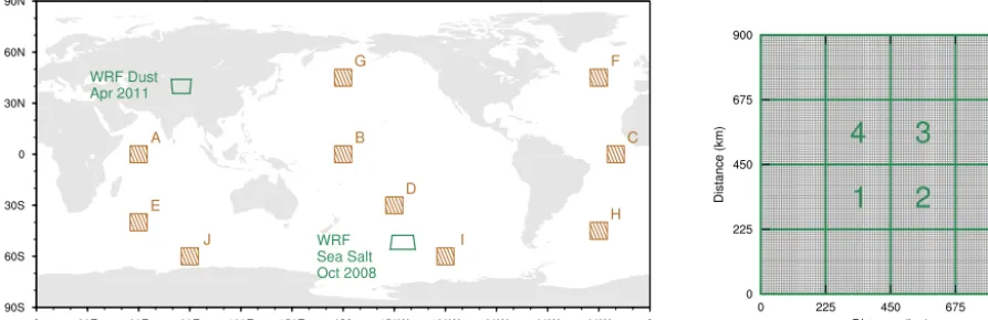
Figure 1.Left panel indicates the two 900km_⇥900kmWRF domains (green), and the ten 10 lat⇥10 lon regions (brown) in which the estimated sub-grid wind variabilities are evaluated in Fig. 8. Right panel shows the four imagined 225kmgrid boxes (label as 1–4) in each of

the WRF domains shown in the left panel. The 225kmgrid boxes are used for the offline estimates in Figs. 4 and 6, as well as the evaluations in Figs. 9 and 11.

of the optimal saltation particles which are assumed to have diameters of 75µm (Zender et al., 2003).u⇤talso depends

on soil moisture and ambient air density. The PFT-dependent friction velocity u⇤sj represents the Owen effect (Owen ,

260

1964). In the default model (i.e., without wind SGV), it is calculated using

u⇤sj =

8 < :

u_⇤j + 0.003U 2 10j

⇣

1 u⇤t u⇤j

⌘2

u_⇤j >u⇤t u⇤j, u⇤j < u⇤t

(6)

The friction velocityu⇤j and the 10mwind speedU10j are functions of surface wind speed, boundary layer stability,

265

and characteristics of the land surface. Like in earlier studies (e.g., Godfrey and Beljaars, 1991; Lunt and Valdes, 2002), in order to take into account the enhancement of mean wind speed by dry convective eddies, in the default CAM5, the calculation of surface heat, moisture and tracer fluxes over

270

land uses the following approximation for the grid-box mean surface wind speed:

Uadj=

q

|v_|2₊ 2

U,d. (7)

Here U,dis the standard deviation of sub-grid wind speed associated with dry convective eddy (details are given in

275

Sect. 4.2.2).Uadj is used in the calculation ofU10 andu⇤,

which not only affects Eq. (6) and hence the dust emissions, but also all other flux calculations that useU10 andu⇤ over

land. On the other hand, the adjustment (Eq. 7) is not applied over the ocean, thus does not affect the sea salt emission in

280

the default model.

2.5 Incorporating surface wind variability in emissions calculations

Equations (2)–(6) reveal that the parameterized sea salt and dust emissions are directly affected by the 10mwindU10and

285

the friction velocityu⇤, both of which depend on the surface

wind speed. In this study, the basic approach to introducing sub-grid scale wind variability in the calculation of aerosol emissions is to (1) assume a Weibull PDF for surface wind speed, and calculate the Weibull PDF parameters from

exist-290

ing model quantities, (2) obtain multiple samples of surface wind speed within each GCM grid box, (3) calculate the sea salt and dust emissions for each sample, and (4) provide the average fluxes to the host GCM.

Using a generic notation, we assumeMsamples of surface

295

wind speed can be obtained in a GCM grid box (i.e.,Uiwith

i= 1,···, M), each of which represents an area fractionwi,

and has a corresponding 10mwindU10i and a friction ve-locityu_⇤i. The grid-box mean sea salt emission flux is then calculated by

300

F=AocnE

X

i

wiU10i3.41. (8)

For dust, we note that the friction velocityu_⇤ is strongly affected by land surface characteristics, which has partially been taken into account (in the default model) by distinguish-ing different PFTs. This is different from the dust emission

305

parameterization used in many other global aerosol-climate models (e.g. ECHAM5-HAM2 described in Zhang et al., 2012), in which the calculation of the friction velocity often neglects the impact of sub-grid variation of vegetation type. On the other hand, for a single PFT in a grid cell, u⇤ can

310

still have strong SGV because of the inhomogeneity in sur-face wind speed. In this study we take multiple sursur-face wind

Figure 1. Left panel indicates the two 900 km×900 km WRF domains (green), and the ten 10◦lat×10◦long regions (brown) in which the estimated sub-grid wind variabilities are evaluated in Fig. 8. Right panel shows the four imagined 225 km grid boxes (label as 1–4) in each of the WRF domains shown in the left panel. The 225 km grid boxes are used for the offline estimates in Figs. 4 and 6, as well as the evaluations in Figs. 9 and 11.

according to White (1979). Note that there were typograph-ical errors in the original Eq. (22) of White (1979), and in Eq. (10) of Zender et al. (2003). Our model uses the formula corrected by Namikas and Sherman (1997, Eq. 3 therein):

Qsj=



 

 

csρau3∗s_j g

1− u∗t u∗sj

1+ u∗t u∗sj

2

, u∗sj > u∗t

0, u∗sj6u∗t.

(5)

cs denotes the saltation parameter (time-invariant and glob-ally constant).ρais air density, andgis gravity. The thresh-old friction velocity u∗t is determined by the size and den-sity of the optimal saltation particles, which are assumed to have diameters of 75 µm (Zender et al., 2003). u∗t also de-pends on soil moisture and ambient air density. The PFT-dependent friction velocity u∗sj represents the Owen effect (Owen, 1964). In the default model (i.e., without wind SGV), it is calculated using

u∗sj =



 

 

u∗j +0.003U 2 10j

1−u∗t u∗_j

2

u∗j>u∗t

u∗j, u∗j < u∗t.

(6)

The friction velocity u∗j and the 10 m wind speed U10j are functions of surface wind speed, boundary layer stability, and characteristics of the land surface. Like in earlier studies (e.g., Godfrey and Beljaars, 1991; Lunt and Valdes, 2002), in order to take into account the enhancement of mean wind speed by dry convective eddies, in the default CAM5, the calculation of surface heat, moisture and tracer fluxes over land uses the following approximation for the grid-box mean surface wind speed:

Uadj=

q

|v|2_+σ2

U,d. (7)

HereσU,dis the standard deviation of sub-grid wind speed associated with dry convective eddy (details are given in

Sect. 4.2.2).Uadj is used in the calculation ofU10 andu∗, which not only affects Eq. (6) and hence the dust emissions, but also all other flux calculations that useU10andu∗over land. On the other hand, the adjustment (Eq. 7) is not applied over the ocean; thus, it does not affect the sea salt emission in the default model.

2.5 Incorporating surface wind variability in emissions calculations

Equations (2)–(6) reveal that the parameterized sea salt and dust emissions are directly affected by the 10 m windU10and the friction velocityu∗, both of which depend on the surface wind speed. In this study, the basic approach to introducing sub-grid-scale wind variability in the calculation of aerosol emissions is to

1. assume a Weibull PDF for surface wind speed, and cal-culate the Weibull PDF parameters from existing model quantities

2. obtain multiple samples of surface wind speed within each GCM grid box

3. calculate the sea salt and dust emissions for each sample 4. provide the average fluxes to the host GCM.

Using a generic notation, we assumeMsamples of surface wind speed can be obtained in a GCM grid box (i.e.,Ui with

i=1,· · ·, M), each of which represents an area fractionwi,

and has a corresponding 10 m windU10i and a friction ve-locityu∗i. The grid-box mean sea salt emission flux is then calculated by

F =AocnE

X

i

wiU103.i41. (8)

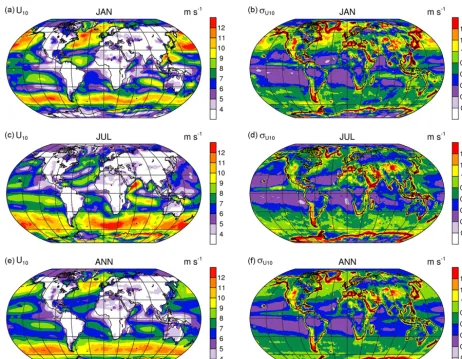
Figure 2. Grid-box average (left column) and sub-grid standard deviation (right column) of the 10 m wind speed, diagnosed on an imagined 2◦×2◦horizontal grid from the ECMWF 15 km global analysis of the year 2011. From top to bottom: January average, July average, and annual mean. See Sect. 3 for further details.

been taken into account (in the default model) by distinguish-ing different PFTs. This is different from the dust emission parameterization used in many other global aerosol-climate models (e.g., ECHAM5-HAM2 described in Zhang et al., 2012), in which the calculation of the friction velocity often neglects the impact of sub-grid variation of vegetation type. On the other hand, for a single PFT in a grid cell, u∗ can still have strong SGV because of the inhomogeneity in sur-face wind speed. In this study we take multiple sursur-face wind samples (Ui, i=1,· · ·, M) for each PFT, calculateu∗sj,iand

Qsj,i in analogy to Eqs. (6) and (5), respectively, then calcu-late the grid-box mean dust emission flux as a weighted sum over all PFTs and all surface wind samples, i.e.,

F =X

j

Aj X

i

wj,iFj,i !

. (9)

The strategy of doing multiple emission calculations in each grid box is similar to that used by Grini and Zender (2004) and Cakmur et al. (2004), although in our work the

wind speed samples are derived differently. The details are explained in Sects. 4 and 5. Before describing the method for estimating sub-grid wind variability, we first present in the next section a diagnostic analysis of the impact of sub-grid wind on aerosol emission, assuming that the sub-grid wind variability is already known.

3 Offline estimate of the impact of wind variability on emissions

This section addresses the first science question listed in Sect. 1, assuming that the sub-grid variability of surface wind is known to sufficiently high accuracy. Applying a method similar to those used in many recent studies on resolu-tion sensitivities of parameterized physical processes (e.g., Arakawa et al., 2011), we use high-resolution wind data and derive the surface wind statistics in imagined grid boxes that are roughly 200 km by 200 km in size.

(a) (b)

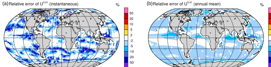
Figure 3. Relative error ofU₁₀3.41over the ocean, caused by ignoring sub-grid wind variability. The quantity shown is the relative error of Eq. (10) with respect to Eq. (11), calculated on an imagined 2◦×2◦horizontal grid using the ECMWF 15 km global analysis. Left panel shows the instantaneous results at an arbitrarily chosen time (00:00 GMT on 1 January 2011). Right panel shows the relative error of the year 2011 annual mean.

Figure 4. (a–b) Time series of the error ofU₁₀3.41 in the four 225 km×225 km grid boxes in the WRF domain over the Southern Ocean (cf. Fig. 1 and Sect. 3). The absolute and relative errors are calculated for Eq. (10) assuming Eq. (11) is the “truth”. (c) Joint frequency distribution of the relative and absolute errors. All the four time series shown in panels (a) and (b) are considered as one sample for the calculation.

Two sources of high-resolution data are used. The first data set contains 1 year (2011) of the 6-hourly opera-tional analysis from the European Center for Medium-range Weather Forecasts (ECMWF). The horizontal resolution is

TL1279, corresponding to grid spacings of about 15 km.

A special advantage of this data set is its global coverage, which is important for estimating the impact of wind SGV on sea salt emission. Our imagined coarse-resolution grid is a 2◦lat×2◦long mesh. Each grid box overlaps about 200 points on the TL1279 grid. The averaging from

fine-resolution grid points to coarse-fine-resolution boxes uses an area weighting that takes into account fractional contributions of the ECMWF grid cells in each 2◦imagined grid box.

The second wind data set includes two regional model simulations conducted with the WRF (Weather Research and Forecasting) model v3.4.1 (Skamarock and Klemp,

2008) at 3 km resolution: one for October 2008 with a 900 km×900 km domain centered at 52◦S, 145◦W over the Southern Ocean, and one for 1–7 April 2011 with a 900 km×900 km domain centered at 40◦_{N, 85}◦_{E over} western China near the Taklamakan Desert (Fig. 1). Both simulations used the CAM5 physics suite implemented in WRF by Ma et al. (2014). The meteorological initial con-ditions and lateral boundary concon-ditions are derived from ECMWF analysis at 6 h intervals. For the calculations dis-cussed in this section and in Sect. 4, each WRF domain is divided into 16 imagined grid boxes of 225 km spacing, and only the four inner boxes are used in order to avoid potential impacts of boundary effects on the regional model simula-tions (Fig. 1b).

K. Zhang et al.: Sub-grid wind-driven aerosol emissions in CAM5 613

(a) (b)

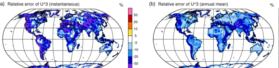
Figure 5. As in Fig. 3 but for the relative errors ofU₁₀3 over land. The errors are calculated for Eq. (12) assuming Eq. (13) is the truth. Figure 5.As in Fig. 3 but for the relative errors ofU3

10over land. The errors are calculated for Eq. (12) assuming Eq. (13) is the “truth”.

Figure 6.As in Fig. 4 but for the WRF simulation over Western China, and for the error ofU3

10. The errors are calculated for Eq. (12)

assuming Eq. (13) is the “truth”.

tion between the grid-box mean and sub-grid variability

dicate that the mean wind alone is not a good predictor of

variability.

Based on Eq. (8), the impact of sub-grid wind variability

on the parameterized sea salt emission can be estimated by

comparing the following two quantities for each grid box:

U

=

U

,

(10)

U

=

X

i

w

U

.

(11)

The subscripts “m” (for “mean”) and “r” (for “reference”)

denote the quantities calculated without and with the

consid-eration of sub-grid wind variability, respectively. The

tive differences diagnosed from the ECMWF data are shown

for an arbitrarily chosen time instance in Fig. 3a, and for the

annual mean in Fig. 3b. For about 75

%

of the ocean grid

points, the relative difference is small (less than 10

%

in

magnitude). On the other hand, local differences exceeding

30

%

in magnitude cover about 8

%

of the ocean area. The

largest spatial variances are mainly associated with

precipi-tation events driven by convective activities.

A similar comparison is presented using the WRF

simula-tion over the Southern Ocean. In Fig. 4a-b, results are shown

for the four 225

km

grid boxes located at the center of the

WRF domain, presented as time series for the entire

simula-tion period (October 2008). In Fig. 4c, the joint frequency

distribution of the relative and absolute errors are shown,

with all four grid boxes considered together. Although the

grid spacing of the WRF simulation is a factor of five smaller

than that of the ECMWF analysis, the relative differences

be-tween

U

m

and

U

are similar: most of the time,

U

calculated from the grid-box mean wind speed agrees within

5

%

with the reference result (

U

r

); There are events

ring every 3–5

days

during which the relative discrepancies

can increase to 30 to 50

%

, but the absolute differences

are generally small.

To get an estimate of the impact of sub-grid wind

variabil-ity on dust emission, we start from Eq. (5) and assume there

is only one PFT in each coarse-resolution grid box. Since the

(a)

(b)

(c)

Figure 6. As in Fig. 4 but for the WRF simulation over western China, and for the error of U₁₀3. The errors are calculated for Eq. (12) assuming Eq. (13) is the truth.

and sub-grid standard deviation ofU10on the 2◦coarse mesh. The statistics were first calculated from the 15 km ECMWF data at 6-hourly intervals, then temporally averaged to give the January, July, and annual averages. Over the ocean, grid-box mean wind and sub-grid variability are both strong in the storm tracks. In contrast, the trade wind regions have rel-atively strong winds but weak SGV, while the regions with strong tropical precipitation are associated with weak grid-box mean wind and strong spatial variability. Over land the mean wind is generally low, but there is strong spatial inho-mogeneity associated with complex topography (e.g., moun-tains and coastlines). The contrasts in geographical distribu-tion between the grid-box mean and sub-grid variability in-dicate that the mean wind alone is not a good predictor of variability.

Based on Eq. (8), the impact of sub-grid wind variability on the parameterized sea salt emission can be estimated by comparing the following two quantities for each grid box:

U_m3.41=U3₁₀.41, (10)

U_r3.41=X

i

wiU10i3.41. (11)

The subscripts “m” (for mean) and “r” (for reference) de-note the quantities calculated without and with the consid-eration of sub-grid wind variability, respectively. The rela-tive differences diagnosed from the ECMWF data are shown for an arbitrarily chosen time instance in Fig. 3a, and for the annual mean in Fig. 3b. For about 75 % of the ocean grid points, the relative difference is small (less than−10 % in magnitude). On the other hand, local differences exceeding

−30 % in magnitude cover about 8 % of the ocean area. The largest spatial variances are mainly associated with precipi-tation events driven by convective activities.

A similar comparison is presented using the WRF simula-tion over the Southern Ocean. In Fig. 4a–b, results are shown for the four 225 km grid boxes located at the center of the WRF domain, presented as time series for the entire simula-tion period (October 2008). In Fig. 4c, the joint frequency distribution of the relative and absolute errors are shown, with all four grid boxes considered together. Although the

grid spacing of the WRF simulation is a factor of 5 smaller than that of the ECMWF analysis, the relative differences betweenU_m3.41andU_r3.41are similar: most of the time,U₁₀3.41

calculated from the grid-box mean wind speed agrees within 5 % with the reference result (U_r3.41); there are events occur-ring every 3–5 days duoccur-ring which the relative discrepancies can increase to−30 to−50 %, but the absolute differences are generally small.

To get an estimate of the impact of sub-grid wind variabil-ity on dust emission, we start from Eq. (5) and assume there is only one PFT in each coarse-resolution grid box. Since the dominant term (in terms of sub-grid variability) in the for-mula isu3∗, andu∗ is closely related to the 10 m windU10, we further simplify the analysis by comparing

U_m3=U3₁₀, (12)

U_r3=X

i

wiU103i. (13)

It should be pointed out that unlike the actual parameter-ization in the model, this simplified comparison does not take into account the dependence of emission flux on the threshold friction velocity. As can be derived from Eq. (5), the omission will lead to an underestimation of the emission flux and emission error whenu∗s>1.6u∗t, and an overesti-mation whenu∗sis close to or smaller thanu∗t. The purpose of using the simplified formulae here is to give a first, rough estimate of the impact of wind SGV. More accurate compar-isons using the CAM5 model with the Zender et al. (2003) parameterization are presented in Sect. 5.

Figures 5 and 6 present the emission errors caused by us-ing the grid-box mean wind speed, diagnosed accordus-ing to the simplified Eqs. (12) and (13) using the ECMWF anal-ysis and the WRF simulation. The relative differences are typically between −10 and −50 % in western China, cen-tral Asia, and western United States, which are important dust source regions (Fig. 5). The WRF simulation in west-ern China contains a strong-wind event around day 4, during which the relative differences betweenU_m3andU_r3increase to

−20 to−50 %. The frequency distributions shown in Figs. 4 and 6 indicate that large absolute errors occur considerably more often for dust emission than for sea salt emission.

The results shown above suggest that considering only the grid-box mean wind speed can lead to substantial inaccu-racies on the parameterized aerosol emission, especially for dust. For a more accurate estimate of the impact of surface wind SGV on aerosol emissions and climatology in CAM5, it is worth implementing multiple emission calculations us-ing different wind samples. In the next section, we present and evaluate a method that derives wind speed samples using GCM-predicted mean states.

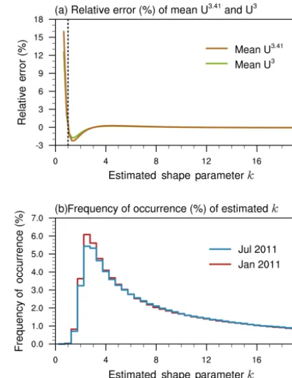
Figure 7. (a) Relative error inU₁₀3.41andU₁₀3 as a result of estimat-ing the shape and scale parameters of a Weibull distribution usestimat-ing Eqs. (15) and (16). (b) Histograms of the Weibull shape parameter kestimated with Eq. (15) using 6-hourly ECMWF analysis of Jan-uary and July 2011 for imagined 2◦grid boxes. Further details can be found in Sect. 4.1.

4 Approximating sub-grid wind variability

Earlier studies have shown that the Weibull distribution is useful and appropriate for representing the temporal fre-quency distribution of wind speed, for example for wind en-ergy applications (Justus et al., 1978). Ridley et al. (2013) showed that if the sub-grid variance inside a GCM grid box is known, using the Weibull PDF to represent the sub-grid variability of surface wind speed can help improve the ac-curacy of the emission calculation compared to a simulation that does not account for the SGV. In this section we discuss empirical methods to estimate the sub-grid wind distribution using GCM-predicted physical quantities.

4.1 Weibull distribution

Assuming the wind speedU is a random variable, the PDF of a Weibull distribution can be written as

p(U;k, c)=

k c

U c

k−1

e−(U/c)k, (14)

wherekis the shape parameter andcthe scale parameter.k

deviation (σU) using method 3 of Justus et al. (1978), i.e.,

k= U

σU !1.086

, (15)

c= U

0(1+1/ k), (16)

where0is the Gamma function.

We note that kandccomputed from Eqs. (15) and (16) are approximations, which define a new Weibull distribution that features exactly the same mean U but differs from the original distribution in terms of higher moments. To evalu-ate the impact of the parameter estimation error on our study of aerosol emission, we generated a large number of Weibull distributions with the true shape and scale parameters var-ied in the range (0, 20). Figure 7a shows the relative error ofU₁₀3.41andU₁₀3 corresponding to the estimated Weibull pa-rameters. The reference values were derived from the orig-inal Weibull distributions with known (i.e., true) k and c. The relative errors are independent of the scale parameterc; thus, only relationships to the shape parameter are presented here. (The relative errors are plotted against the estimatedk, rather than the known true value, to allow for straightforward comparison with Fig. 7b; see below.) Figure 7a shows that the relative errors in U₁₀3.41 andU₁₀3 are both small (within 3 %) when the estimated shape parameter is larger than 1. The errors are negligible whenk >3 (corresponding to neg-ative skewness or very small positive skewness). Fork <1, Eqs. (15) and (16) give much less accurate results, but this is expected to have negligible impact on our results presented later in this paper, because as Fig. 7b indicates, the shape pa-rameters of 2◦grid boxes derived from the ECMWF analysis rarely drop below 1. The two histograms in Fig. 7b were cal-culated from 6-hourly global data of January and July 2011. The percentages of grid boxes with k <1 were 0.036 % in January and 0.025 % in July.

The usefulness of the Weibull distribution for represent-ing the sub-grid wind variability can be seen in a diagnostic comparison similar to those shown in Figs. 3 and 5. Using the 15 km ECMWF data, we derive the grid-box mean and sub-grid standard deviation of the 10 m wind speed (U10and

σU10, respectively) on the 2

◦_{coarse mesh, and calculate the} shape and scale parameterskandcusing Eqs. (15) and (16). The central 99 % of the resulting Weibull PDF is then di-vided into 100 bins. The discrete PDFs are used in Eqs. (11) and (13), withwibeing the frequency of occurrence of bini.

The errors inU₁₀3.41 andU₁₀3 caused by using the Weibull distribution instead of the true sub-grid wind distribution (not necessarily Weibull) turn out to be very small (not shown). In terms of both instantaneous values and annual averages, the use of Weibull distribution typically gives errors of less than 2 % over the ocean and less than 5 % over land. These errors are substantially smaller than in the case when only the grid-box mean values are included in the calculation (Figs. 3 and

5 in the previous section). This suggests that with sufficiently accurate estimates of the parameters, the Weibull distribution is a very good approximation of the spatial variability of the near-surface wind speed.

Fitting the Weibull distribution as discussed above requires the sub-grid mean and standard deviation of wind speed. Typ-ically, a GCM provides only the grid-box mean wind vector

v. The magnitude of that mean wind vector,|v|, is an under-estimate ofU, while a better approximation can be obtained using the standard deviationσU. ObtainingσU is thus a key

step for fitting the sub-grid wind speed distribution. Consid-ering that the SGV is caused by parameterized physical pro-cesses and sub-grid-scale features such as complex topog-raphy, the ideal sources of information onσU would be the

corresponding parameterizations. For example, the represen-tation of cold pool in the unified convection scheme (UNI-CON; Park, 2014) might be used to estimate the SGV caused by mesoscale organized flow associated with deep convec-tion. A high-order turbulence scheme might provide useful predictions of the Raynold’s stress to help estimate the wind variability related to turbulence. Since these are not yet avail-able in the standard version of CAM5, we resort to empirical estimates ofσU as discussed next.

4.2 Empirical estimate ofσU

Relatively simple methods have been used in the literature to estimate the parameters needed to determine a Weibull distri-bution for wind speed. For example, Grini and Zender (2004) and Capps and Zender (2008) used method 5 of Justus et al. (1978), i.e.,

k=CpU (17)

withC being a constant. In the work of Grini and Zender (2004),Cwas set to 0.94 to approximate the sub-grid wind variability on land. Their formula effectively estimatesσU

fromUusing

σU=1.059U

0.54

. (18)

Some other studies on dust emission used an even simpler method by assuming k is constant over land (e.g., Menut, 2008).

In this work we are interested in global emissions of sea salt and dust. Preliminary investigations indicated that con-stantkor Eq. (17) with constantC gave reasonable results over certain locations over land but had large regional dis-crepancies, and both methods were unsatisfactory over the ocean. Below we use a set of empirical formulae to relateσU

to four types of physical processes: i. neutral/stable turbulent mixing (σU,t) ii. dry convective eddy (σU,d)

iii moist convective eddy over the ocean (σU,m)

iv. mesoscale flow associated with sub-grid orography over land (σU,l).

The total sub-grid standard deviation of surface wind speed is defined as

σU = q

σ_U,2_t+σ_U,2_d+σ_U,2_m+σ_U,2_l. (19) Among those processes, the first two are associated with spatial scales that can only be resolved by large-eddy sim-ulations (LESs) or Direct Numerical Simsim-ulations (DNSs). Such simulations, and the related observational data, are still very limited in terms of spatial and temporal coverage (e.g., Dipankar, 2015). We do not have sufficient amount of new, high-resolution data to analyze these processes or evaluate parameterizations. We thus choose to use results from earlier studies in the literature.

Moist convective eddies and orography-related mesoscale flows are partially resolved in the ECMWF 15 km analysis. Since the analysis is available for 2 years (2011 and 2012), we use the first year to derive empirical relationships for es-timating σU,m andσU,l, then use the second year to evalu-ate the fitting. The accuracies of the derived relationships are inherently constrained by the resolution of the analysis data. The fact that the 15 km resolution is too coarse to re-solve neutral/stable turbulence and dry convective eddies is an advantage for us, in that the sub-grid wind variability esti-mated from the ECMWF analysis do not include the impact of neutral/stable turbulence and dry convective eddies. There is hence no double counting betweenσU,mandσU,l derived from the 15 km analysis, and theσU,tandσU,destimated us-ing process-based formulation. One might still raise the con-cern that the 15 km resolution is also too coarse to fully re-solve moist convection and fine-scale topography effect. Al-though the concern is legitimate, we show in the section that the derived relationships are able to give quite accurate emis-sion estimates when evaluated against the WRF simulations (3 km resolution). This provides good confidence in the em-pirically fitted relationships, at least for important regions of sea salt and dust emission that are of interest for our pur-poses. In the future, it will be useful to further evaluate and update the sub-grid wind variability parameterizations us-ing additional high-resolution data (when they become avail-able). Another useful and challenging research topic is to construct process-based parameterizations instead of empiri-cal fitting as discussed here.

4.2.1 Neutral/stable turbulent mixing

To consider the influence of turbulent mixing in a neutral or stable boundary layer, we follow ECMWF (2004) and esti-mate the resulting wind variability using

σU,t=

(

2.29u∗(|v|) whenFθv60

0 whenFθv>0.

(20)

HereFθv is the surface buoyancy flux (unit: m

2_s−1₎ de-fined in Zeng et al. (2002),θv is the virtual potential tem-perature (unit: K),u∗(|v|)is the friction velocity diagnosed from the speed of the grid-box mean wind|v|. In Eq. (20) the strength of turbulence is represented by the friction ve-locityu∗, not the TKE (cf., e.g., Cakmur et al., 2004). This choice results from the experience that TKE is not provided by all GCMs, and, when available, its characteristic value and spatio-temporal distribution can differ substantially from model to model.

4.2.2 Dry convective eddies

The contribution of dry convective eddies to sub-grid wind variability is estimated using a formulation recommended by Redelsperger et al. (2000) and Lunt and Valdes (2002):

σU,d=







0 whenFθv60

_{gH F}

θv θv

1₃

whenFθv >0,

(21)

His the boundary layer height (unit: m), andgis gravity. Note that by using the surface buoyancy fluxFθv as a

cri-terion, we consider contributions from either neutral/stable turbulence mixing (Eq. 20) or dry convective eddies (Eq. 21), but not both, for the purpose of avoiding double counting. 4.2.3 Moist convective eddies over the ocean (σU ,m)

For the influence of moist convective eddies and downdrafts, Redelsperger et al. (2000) constructed an empirical formula based on two 2-D cloud-resolving model (CRM) simulations that covered 1 week in time and 512 km across the horizontal domain, with a horizontal resolution of 2 km. Their formula uses the surface precipitation rateP (mm day−1) as the pre-dictor for sub-grid wind variability:

σU,m=ln(1+6.69P−0.47P2) . (22)

In this study we are interested in sea salt emissions, the main sources of which are located in the storm tracks (i.e., mid-latitudes). Given that the Redelsperger et al. (2000) equation was derived from simulations of tropical deep con-vection with very limited temporal and spatial coverage, it was unclear whether the same relationship would be appro-priate for our purpose. We attempted to derive a similar re-lationship using the ECMWF 15 km analysis of 2011, and indeed found it difficult to obtain one good formula for all latitudes. The best-fit formula for a 2◦×2◦ GCM grid has the form

σU,m=

(

0.95 ln(1+4.01

√

P +0.31P2) (ocean)

0 (land), (23)

where

P =

(

Pstrat+conv where SST<295 K, 0.2Pstrat+conv where SST>295 K.

Figure 8. Time series of the sub-grid standard deviation of U10 (m s−1) in January 2012 averaged over the 10◦×10◦hatched boxes in Fig. 1. Dashed black curves are directly diagnosed from the ECMWF surface wind data. Solid blue and red curves are the σU,mcalculated using the ECMWF precipitation rates and the em-pirical formulas of this study (Eq. 23) and Redelsperger et al. (2000) (Eq. 22), respectively.

The SST criterion essentially distinguishes the tropics and mid-latitudes.

Figure 8 presents time series of the sub-grid standard de-viation of surface wind speed calculated with Eqs. (22) and

Figure 9. As in Fig. 8 but evaluating Eqs. (23) and (22) using the WRF simulation over the Southern Ocean. The domain of the WRF simulation and the location of the four imagined 225 km×225 km grid cells are illustrated in Fig. 1.

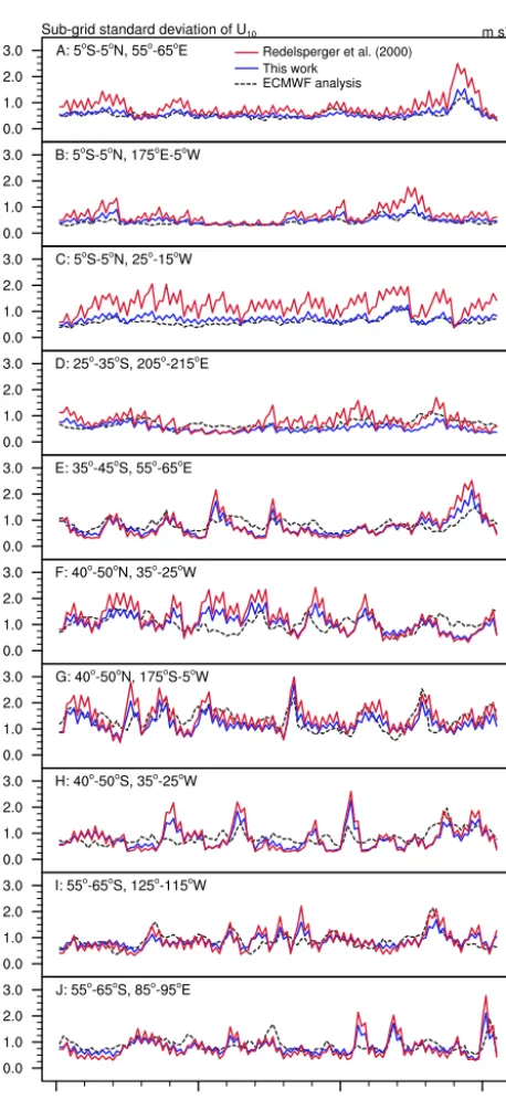
(23), and the values directly derived from the ECMWF anal-ysis. The results are shown for January 2012 for a few arbi-trarily chosen 10◦×10◦regions (cf. Fig. 1). Results in other months are similar and thus not shown. In the low latitudes, the Redelsperger et al. (2000) formula predicts considerably higher wind variability than both our fitting and the ECMWF analysis. This is consistent with our expectations since the CRM simulations, which the Redelsperger et al. (2000) is based on are capable of resolving substantially more convec-tive activity than the ECMWF analysis. In the mid-latitudes, however, the two formulae give very similar estimates, and both agree reasonably well with the ECMWF analysis.

Given the 15 km resolution, one might still question whether the ECMWF analysis is an appropriate reference for the evaluation here. To address this issue, Fig. 9 evaluates the two empirical formulae by comparing the estimates with the WRF simulation over the Southern Ocean. For each of the 225 km×225 km box at the center of the WRF domain, the diagnosed sub-grid variability is shown in black and the estimated values in red and blue. Again, the two empirical formulae give very similar results. Both are able to capture the mean wind variability over the simulated period, and the most frequently occurring high and low values, although the strongest peaks are underestimated. The Redelsperger et al. (2000) formula gives larger peak values than our fitting de-rived from the ECMWF data, but the differences are rela-tively small. On the whole, the two empirical formulae have similar predictive skills. This provides confidence that they

Figure 10. Geographical distribution of the coefficientD(unitless) derived for a 2◦lat×2◦long GCM grid using the ECMWF 15 km analysis of the year 2011 and Eq. (26). The locations with no results are either covered by land ice or lake, or associated with leaf area indices (LAI) larger than 0.3 throughout the year; thus, cannot have dust emission according to the parameterization of Zender et al. (2003) and the land surface characteristics data used in the CAM5 simulations in this paper. The black boxes correspond to the panels in Fig. 11 in which time series of sub-grid wind variability are analyzed.

are both suitable for estimating sub-grid wind variability in mid-latitudes. In principle one could also conduct and ana-lyze a high-resolution WRF simulation of deep convection to get more insight into the discrepancies in the tropics be-tween our fitting and the Redelsperger et al. (2000) formula. Such a comparison is not included in this paper because as discussed later in Sect. 5.3, CAM5 simulations indicate that sea salt emission fluxes are very low in the tropics; even with Redelsperger’s formula, which gives stronger wind variabil-ity than our fitting does, the absolute increases in sea salt emission and loading remain negligible when compared with higher latitudes.

4.2.4 Mesoscale flows over land (σU,l)

The sub-grid wind speed variance diagnosed from the ECMWF analysis (Fig. 2 in Sect. 3) indicates clearly that over land, the strongest variabilities are associated with com-plex topography. Such disturbances can be caused by pure dynamical effects, but they can also involve moist processes (e.g., cumulus convection), and thus are difficult to parame-terize. A preliminary investigation showed that for individual locations, the sub-grid wind variance is strongly correlated with the grid-box mean wind speed. We therefore follow the idea of Eq. (17) but, unlike earlier studies in the literature, make the coefficient a location-dependent and time-invariant parameter. Also, in order to have a coefficient that scales with the SGV, we use the reciprocal of the coefficientC(i.e.,

D=1/C) in the equations and figures below, i.e.,

k (x, y, t )=

q

U (x, y, t )

D (x, y) , (25)

where x andy denote longitude and latitude, respectively. The parameterDis derived from the ECMWF analysis using the following procedure: first, for each 2◦grid cell, calculate

the grid-box mean wind speed and the sub-grid standard de-viation; second, calculatekusing Eq. (15); third, derive the time-invariantCusing temporally averagedUandk, i.e.,

D (x, y)=

n P

t=1

q

U (x, y, t )

n P

t=1

k (x, y, t )

. (26)

The time indext goes through all 6-hourly samples of the year 2011. After determiningD, the standard deviation of sub-grid wind speed is calculated by

σU,l=

(

0 (ocean)

D|v|0.5861/1.086 (land). (27)

In Fig. 10, the coefficient D derived from the 2011 ECMWF analysis is shown in potential dust source regions. The spatial pattern ofDis strongly correlated with topogra-phy. As a result,Dshows substantial regional variation: Asia and South America have large areas with D >0.5, while most grid cells in Australia and North Africa haveD <0.5. Within these regions, the coefficient also has substantial spa-tial variation at the thousand-kilometer scale.

Figure 11. Time series of the sub-grid standard deviation ofU10 (m s−1) in January 2012 in the 2◦lat×2◦long grid cells indicated by red boxes in Fig. 10. Dashed black curves are results derived from the ECMWF 15 km analysis. Red curves are results estimated using Eq. (27) withD=1.06. Blue curves are also estimates using Eq. (27), but with location-dependentDcalculated from Eq. (26).

(Fig. 11d–f), Australia (Fig. 11g and h), and North America (Fig. 11i–h). The empirical formula with spatially varying

D(blue lines in Fig. 11) is able to capture the characteristic magnitude of the wind variability, as well as main features of the temporal evolution. In contrast, the wind variability

Figure 12. As in Fig. 11, but for the four 225 km boxes at the center of the WRF domain near the Taklamakan Desert. TheDvalues used for the blue curves are derived from the ECMWF analysis of year 2011 for 2◦lat×2◦long grid cells that are closest to the 225 km boxes.

estimated withD=1.06 is about 100–200 % larger than the analysis in Australia, and more than a factor of 3 stronger in northwest Africa, where the topography is relatively flat.

It is also worth noting that for our empirical estimates shown in Fig. 11, the coefficientDis derived from the anal-ysis of 2011 but applied to the year 2012. The agreement be-tween the empirical estimate and the analysis suggests that the relationship between grid-box mean wind speed and sub-grid wind variance is not strongly affected by interannual variability of the general circulation.

In Fig. 12, estimates of sub-grid wind speed variability based on constant or locally fitted D are evaluated using the 7-day WRF simulation near the Taklamakan Desert. The black curves in the figure indicate wind variability in the four 225 km×225 km boxes at the center of the WRF do-main (cf. Fig. 1), derived from the 3 km model output. The red curves are the estimates based onD=1.06. The results shown in blue are calculated using theDvalues fitted from the ECMWF analysis for the 2◦lat×2◦long grid cells that are closest to the 225 km boxes. Although the ECMWF anal-ysis does not resolve scales smaller than 15 km, the coeffi-cientD derived from the ECMWF data leads to very rea-sonable estimates of wind variability compared to the 3 km WRF simulation, providing confidence in the ECMWF anal-ysis and the fitted D values in regions of fine-scale topo-graphical features. It should be mentioned that the reference wind data used here have limitations in terms of the spatial and temporal coverage, and the horizontal and vertical reso-lutions. Physical mechanisms of wind variabilities and dust emission in the real world and their representation in numeri-cal models are highly complex. For example, Marsham et al. (2011) showed that models with parameterized or resolved convection can give different timings of summer dust uplift in West Africa. The parameterization of wind SGV presented in this paper is very simple and empirical. Process-based

4. Calculate the total sub-grid-scale variability using Eqn. (19).

6. Calculate shape and scale parameters using Eqs. (15) and (16).

7. Generate a Weibull distribution using Eq. (14). Discretize the central 99% into

100 bins.

8. For each bin, calculate sea salt emission (Eq. 2) and dust emission

(Eqs. 4–6) using mean wind speed of the

bin instead of the grid cell average.

9. Integrate the emission fluxes over the distribution (100 bins).

5. Estimate the sub-grid mean wind speed using Eq. (28).

1. For a grid cell, get the resolved surface wind speed and the precipitation rates.

10. Calculate the area-weighted sum of emissions fluxes of all PFTs in the grid cell.

2. For the jth PFT, get the PFT-specific 10 m wind speed, friction velocity, boundary layer height, virtual potential temperature,

and surface buoyancy flux.

3. Calculate the four components of sub-grid-sale wind variability using Eqs. (20),

(21), (23), (24), and (27)

Next PFT

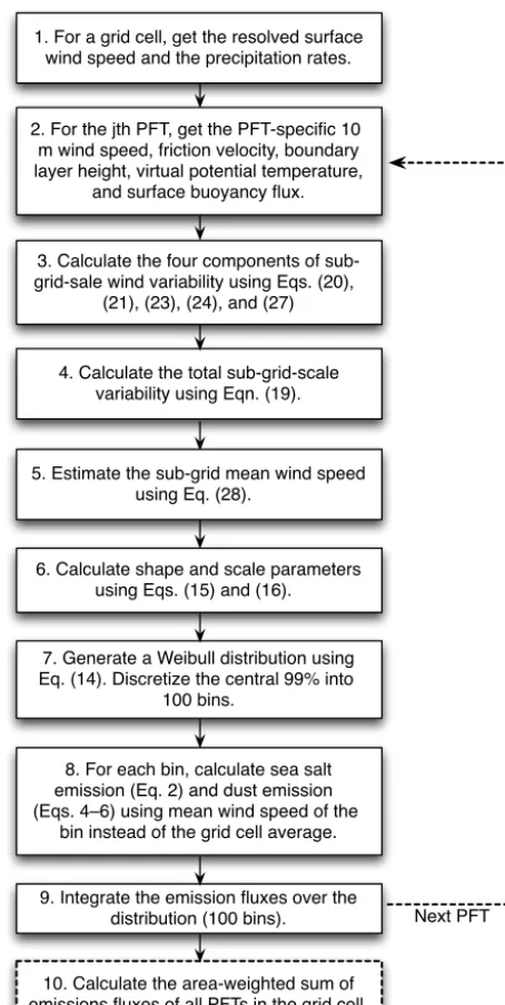
Figure 13. Flowchart illustrating the implementation of wind-distribution-based sub-grid emission calculations in CAM5. Dashed lines indicate steps that are only relevant for the dust emission cal-culation.

resentation of different dust emission mechanisms is a topic for future study.

4.3 Implementation in CAM5

The wind-distribution-based emission calculations are im-plemented in CAM5, as illustrated in Fig. 13.

In the previous subsections we have shown that the Eqs. (23), (24), (26), and (27) can provide very good esti-mates of the sub-grid wind speed variability when compared with the ECMWF analysis and WRF simulations. These

em-pirical relationships are combined with Eqs. (20) and (21) to provide an estimate of the total sub-grid variance of surface wind speedσU using Eq. (19).

Given the GCM predicted grid-box mean wind vectorv

and the estimated σU, we assume that the sub-grid mean

wind speed can be approximated by

U≈

q

|v|2_+σ2

U. (28)

This is similar to Eq. (7), which originated from Zeng et al. (2002), but takes into account additional sources of wind speed SGV.

U and σU are used in Eqs. (14)–(16) to determine

a Weibull distribution. Surface wind speed samplesUj are

obtained by equally dividing the central 99 % of the Weibull PDF into 100 bins. Sensitivity simulations with a 20 bin Weibull PDF show similar results. From the surface wind speed samples, the corresponding values of 10 m wind speed and friction velocity are derived, and used to calculate the grid-box mean sea salt and dust emission fluxes following Sect. 2.5. If the estimatedσU is smaller than 0.1 m s−1, we

skip the derivation of Weibull PDF and wind samples, and use only the mean wind speed for the emission calculations. The computation cost for the sub-grid treatment is small (less than 3 % of the total simulation cost).

The next section presents a series of CAM5 simulations to quantify the impact of sub-grid wind variability on aerosol emission and the model’s mean climate. For clarification, we note that theσU andU(Eq. 28) described above are applied

only to the sea salt and dust emission parameterizations. As mentioned at the end of Sect. 2.4, the default model uses an adjusted mean wind speed (Eq. 7) for all calculations related to surface fluxes and boundary layer processes over land. This is unchanged in our simulations except for dust emis-sion. We chose not to modify Eq. (7), so as to cleanly sep-arate the impact of sub-grid variability on aerosol emission from the impacts on other physical processes.

5 Impact on aerosol climatology in CAM5

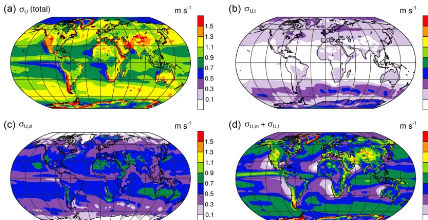
Figure 14. Annual mean sub-grid standard deviation of surface wind speed in CAM5: (a) total (Eq. 19), (b) neutral/stable turbulent mixing (Eq. 20), (c) dry convective eddies (Eq. 21), (d) moist convective eddies over the ocean (Eqs. 23–24) and mesoscale flow over land (Eq. 27).

Table 1. List of CAM5 simulations discussed in Sect. 5. DU and SS refer to dust and sea salt emissions, respectively. “With PDF” means the Weibull distribution of wind speed is used in the emission calculations (cf. Sect. 2.5). “Without PDF” means the enhancement of grid-box mean wind speed is taken into account, but the emission calculations use only the (enhanced) mean wind speed, not the Weibull PDF.

Simulation Source of sub-grid wind variability Dust

Turbulence Dry convective eddy Moist convective eddy Mesoscale flows over topography Emission

(Eq. 20) (Eq. 21) (ocean; Eqs. 23 and 24) (land; Eqs. 26 and 27) factor

NOSG – – – – 0.35−1

CTRL – DU; without PDF – – 0.35−1

EXP1 – DU+SS; with PDF – – 0.35−1

EXP2 DU+SS; with PDF DU+SS; with PDF – – 0.35−1

EXP3 DU+SS; with PDF DU+SS; with PDF DU+SS; with PDF DU+SS; with PDF 0.35−1

EXP4 DU+SS; with PDF DU+SS; with PDF DU+SS; with PDF DU+SS; with PDF 0.57−1

5.1 Online calculated sub-grid-scale wind variability

Annual averages of the estimated sub-grid standard deviation of surface wind speed in CAM5 are presented in Fig. 14a, and the individual components are shown in Fig. 14b–d. Strong SGVs are associated with complex topography, mid-latitude storm tracks, the trade winds, and tropical con-vection. Over the ocean, moist convective eddies are the most important contributor to wind SGV in the tropics (Fig. 14d), while dry convective eddies are the main contrib-utor in the trade wind regions and above warm ocean cur-rents (Fig. 14c). Over the continents, strong wind variabili-ties are associated with sub-grid topography and dry convec-tive eddies (Fig. 14c–d). The impact of neutral/stable turbu-lent mixing is seen mainly in mid- and high-latitude regions (Fig. 14b).

Since the empirical parameterizations forσU,m andσU,l were derived from the ECMWF analysis, the wind SGV in Fig. 14d agree reasonably well with the diagnostic results shown in Fig. 2f for the ECMWF data. The discrepancies over the ocean are attributable to fitting error and differ-ences in the simulated precipitation rates in the two models. Over the continents, the discrepancies are likely caused by the different grid-box mean winds, and the use of a time-independent coefficientD.

5.2 Sensitivity experiments

To evaluate the impact of different sources of wind SGV on the aerosol climatology in CAM5, a series of simulations were performed (Table 1). Experiment CTRL uses the de-fault configuration of CAM5, in which the impact of dry convective eddies is taken into account when estimating the

grid-box mean wind speed Uadj (Eq. 7). Uadj is used for calculating dust emission, while the parameterization of sea salt emission does not account for sub-grid wind variability (Eq. 2). Simulation EXP1 is similar to CTRL in that only dry convective eddies are considered for the wind SGV. The dif-ferences are that (i) the dust emissions are calculated using the wind speed PDF (Eq. 9), and (ii) the same PDF-based method is also applied to sea salt emission (Eq. 8). EXP2 ex-tends EXP1 by adding the contribution of turbulence in neu-tral and stable boundary layers, and EXP3 further extends EXP2 by including the impact of moist convective eddies over the ocean and topography-related small-scale motions over land. For completeness, we also conducted a simulation called NOSG, in which the dust emission is calculated us-ing the speed of resolved wind|v|instead ofUadj; in other words, NOSG does not include any effect of sub-grid wind variability on dust emission. The simulations NOSG, CTRL, EXP1, EXP2, and EXP3 are analyzed in Sect. 5.3 to quantify the contribution of different sources of wind variability to the emission and concentration of sea salt and dust aerosols.

As is shown later in Sects. 5.3, EXP3 features consider-ably stronger dust emission and higher dust loading. In global aerosol-climate models, it is a common practice to apply a constant scaling factor to the dust emission, for the pur-pose of adjusting the global mean dust AOD (aerosol opti-cal depth) as well as the aerosol induced radiative forcing. The default scaling factor in CAM5 for the 2◦finite-volume dynamical core is 0.35−1 (here we follow the form of the scaling factor defined in the model). This value is used in NOSG, CTRL, EXP1, EXP2 and EXP3. When discussing the aerosol climatology in Sect. 5.4, we also present an addi-tional simulation, EXP4, which used the same configuration as EXP3, but the dust emission factor is adjusted to 0.57−1_, which brings the global and annual mean dust emission flux back to the value of the CTRL simulation.

5.3 Contribution of individual sources of wind variability to aerosol emission and optical depth

The impacts of wind SGV on sea salt emission and sea salt AOD at 550 nm are presented in Fig. 15 and Table 2. In the default model (Fig. 15a and b), the strongest sea salt emission occurs in the mid-latitude storm tracks where the majority of the released particles are subsequently removed by precipi-tation. The trade wind regions have moderate emission but very weak wet removal, which leads to high sea salt concen-trations. In the deep tropics, the default model predicts very low emission because the impact of frequent and vigorous convective activity on surface wind SGV is not considered, and the grid-box mean wind speed is low. The low emission, in combination with strong removal associated with the pa-rameterized convection, results in low sea salt AOD in re-gions of strongest convective precipitation.

The impacts of sub-grid wind variability on sea salt emis-sion and optical depth are generally small and spatially

ho-mogenous except in the Inter Tropical Convergence Zone (ITCZ). Taking into account the dry convective eddies (σU,d) leads to a global mean increase of 2.48 % in sea salt emission, and the regional increases are of similar magnitude (EXP1 in Table 2). The impact of neutral and stable turbulence (σU,t) is smaller, less than 2 % both regionally globally (EXP2 minus EXP1 in Table 2). Including moist convective eddies (σU,m) further increases the emission fluxes by about 4 % (EXP3 mi-nus EXP2 in Table 2).

Within the ITCZ, the sub-grid wind variability estimated using our empirical relationships results in 10–35 % in-creases compared to the default model in the annual mean sea salt emission (Fig. 15e), and 10–25 % increases in sea salt AOD (Fig. 15f), mainly due to the moist convective eddies. However, since the resolved-scale wind speed is low in the ITCZ and the wet removal is strong, the contribution of these regions to the global total sea salt budget is small. In terms of global and annual average, the increase in sea salt emis-sion is 7.48 % (Table 2) when comparing EXP3 with CTRL. An additional sensitivity experiment was conducted using the formula of Redelsperger et al. (2000) for the moist convec-tive eddies. The strongest enhancement of sea salt emission exceeded 100 % in the ITCZ, while the resulting emission fluxes remained a factor of 5–10 weaker than in the storm tracks, and the increases in sea salt AOD were generally be-low 50 %. Although the Redelsperger et al. (2000) formula leads to higher wind SGV than our empirical fitting derived from the ECMWF analysis, the impact on the simulated sea salt emission and AOD is still small in terms of global mean and geographical distribution.

The simulated dust emission and optical depth are more sensitive to sub-grid wind variability than sea salt. Table 3 compares dust emissions in the major source regions. In both the control simulation and EXP1, dry convective eddies are taken into account when estimating the grid-box mean wind speed for dust emission; however, using multiple wind sam-ples instead of the mean value leads to about 30 % emission increases in Africa and Asia, and even larger differences in North America and South America (EXP1 in Table 3). This reflects the strong nonlinearity of the dust emission param-eterization. Part of the nonlinearity comes from the fact that the parameterization requires the characteristic friction ve-locityu∗sj to exceed the threshold valueu∗tin order for dust emission to occur (cf. Eq. 5).

Table 2. Simulated annual mean global and regional sea salt emissions (Tg yr−1) for the year 2006. Numbers in parenthesis are the relative differences with respect to the default model (CTRL). Meanings of the simulation short names are explained in Table 1. NOSG and EXP4 are not included here because they are identical to CTRL and EXP3, respectively, in terms of the sea salt emission parameterization.

Simulation Global Northern Hemisphere Southern Hemisphere Tropics (30–60◦N) (30–60◦S) (20◦S–20◦N)

CTRL 5011.3 854.8 2504.8 925.8

EXP1 5135.6 (+2.48 %) 880.5 (+3.00 %) 2547.3 (+1.69 %) 956.0 (+3.27 %) EXP2 5198.9 (+3.74 %) 891.8 (+4.33 %) 2591.3 (+3.45 %) 958.2 (+3.50 %) EXP3 5386.4 (+7.48 %) 929.9 (+8.78 %) 2678.1 (+6.91 %) 996.4 (+7.63 %)

Figure 15. Top row: year 2006 mean sea salt emission flux (kg m−2s−1) and sea salt AOD (unitless) at 550 nm in the nudged CAM5 simulation (CTRL); Second row: differences between EXP3 and CTRL. Bottom row: relative differences between EXP3 and CTRL. In the bottom row, locations that have emission fluxes less than 1×10−12kg m−2s−1or sea salt AOD<0.01 in the CTRL simulation are masked out.

fluxes from the NOSG simulation. Combined with EXP1, these numbers quantify the total impact of dry convective ed-dies. From the table, it is clear that dry convective eddies and mesoscale flows associated with sub-grid-scale topography are the most important factors that affect dust emission in CAM5.

In Fig. 16, the geographical distributions of annual mean dust emission flux and AOD are shown for CTRL, together with the differences between EXP3 and CTRL. For both the emission and the AOD, there is little change in the global

pat-terns, except that the increases in Australia are considerable smaller than those in Africa and Asia.

5.4 Comparison with AOD observations

The diagnostics above showed that applying the PDF method to take into account sub-grid wind speed variability leads to considerable increases in the emission and loading of dust aerosols. To evaluate how much the increases affect the agreement and discrepancies between model simulation and

Table 3. Simulated annual mean global and regional dust emission (Tg yr−1) for the year 2006. Numbers in parenthesis are the relative differences with respect to the default model (CTRL). The experiment configurations are explained in Table 1.

Simulation Global North Africa East Asia West Asia Australia North America South America (10–30◦N, (30–50◦N, (15–50◦N, (10–40◦S, (10–60◦N, (0–60◦S, 20◦W–40◦E) 80–120◦E) 40–70◦E) 110–140◦E) 30–140◦W) 40–80◦W) NOSG 3365.0 (−14.3 %) 1588.4 (−15.6 %) 551.8 (−13.7 %) 522.4 (−15.6 %) 137.5 (−11.8 %) 1.74 (−24.0 %) 7.57 (−39.4 %)

CTRL 3927.9 1880.7 639.3 619.3 155.9 2.29 12.5

EXP1 5015.5 (+27.7 %) 2447.3 (+30.1 %) 876.0 (+37.0 %) 825.2 (+33.2 %) 149.9 (−3.9 %) 3.76 (+64.4 %) 29.0 (+132.0 %) EXP2 5124.5 (+30.5 %) 2500.6 (+33.0 %) 875.8 (+37.0 %) 848.3 (+37.0 %) 174.2 (+11.7 %) 3.88 (+69.5 %) 29.2 (+133.6 %) EXP3 6027.9 (+53.5 %) 2736.1 (+45.5 %) 1133.8 (+77.4 %) 1048.3 (+69.3 %) 188.0 (+20.6 %) 5.03 (+119.7 %) 45.0 (+259.5 %) EXP4 4024.9 (+2.47 %) 1829.1 (−2.74 %) 798.8 (+25.0 %) 683.7 (+10.4 %) 120.3 (−22.9 %) 3.25 (+42.1 %) 28.0 (+123.5 %)

Figure 16. As in Fig. 15 but for dust emission and dust AOD at 550 nm. The threshold values for masking out differences in the bottom row are 1×10−10kg m−2s−1for emission and 0.01 for AOD.

observation, the simulated AOD at 550 nm is compared with satellite retrievals in dust source regions.

Figure 17 compares the annual mean total AOD at 550 nm against satellite retrievals obtained by the Multi-angle Imag-ing SpectroRadiometer (MISR) in 14 major dust source re-gions (Table 4). The definition and indexing of the 14 rere-gions follow Zender and Kwon (2005). Model data are sampled at the satellite local overpass time of 13:30, and are masked out when the corresponding MISR record indicates missing data. Note that we modified the model source code to