www.geosci-model-dev.net/4/1133/2011/ doi:10.5194/gmd-4-1133-2011
© Author(s) 2011. CC Attribution 3.0 License.
Geoscientific
Model Development
Improved convergence and stability properties in a
three-dimensional higher-order ice sheet model
J. J. Fürst1, O. Rybak1, H. Goelzer1, B. De Smedt1, P. de Groen2, and P. Huybrechts1
1Earth System Sciences & Department of Geography, Vrije Universiteit Brussel, Pleinlaan 2, Brussels, Belgium 2Department of Mathematics, Vrije Universiteit Brussel, Pleinlaan 2, Brussels, Belgium
Received: 21 June 2011 – Published in Geosci. Model Dev. Discuss.: 20 July 2011
Revised: 14 October 2011 – Accepted: 12 November 2011 – Published: 19 December 2011
Abstract. We present a finite difference implementation of
a three-dimensional higher-order ice sheet model. In com-parison to a conventional centred difference discretisation it enhances both numerical stability and convergence. In or-der to achieve these benefits the discretisation of the gov-erning force balance equation makes extensive use of infor-mation on staggered grid points. Using the same iterative solver, a centred difference discretisation that operates exclu-sively on the regular grid serves as a reference. The reprise of the ISMIP-HOM experiments indicates that both discreti-sations are capable of reproducing the higher-order model inter-comparison results. This setup allows a direct compar-ison of the two numerical implementations also with respect to their convergence behaviour. First and foremost, the new finite difference scheme facilitates convergence by a factor of up to 7 and 2.6 in average. In addition to this decrease in computational costs, the accuracy for the resultant veloc-ity field can be chosen higher in the novel finite difference implementation. Changing the discretisation also prevents build-up of local field irregularites that occasionally cause divergence of the solution for the reference discretisation.
The improved behaviour makes the new discretisation more reliable for extensive application to real ice geome-tries. Higher accuracy and robust numerics are crucial in time dependent applications since numerical oscillations in the velocity field of subsequent time steps are attenuated and divergence of the solution is prevented.
Correspondence to: J. J. Fürst ([email protected])
1 Introduction
In general, most large-scale ice sheet models describe ice as a nonlinear viscous and isotropic fluid to capture its de-formation. Their main differences lie in the approximations used in the force balance or Stokes equation. The most comprehensive Full-Stokes (FS) models solve the force bal-ance equation without further simplifications to the underly-ing continuum mechanics (Zwunderly-inger et al., 2007; Hindmarsh, 2004; Jouvet et al., 2009). Although they fully capture the deformational dynamics of ice sheets, their applicability is strongly restricted by computational limitations. Therefore approximations derived from scale analysis have been sug-geted for ice sheet modelling. On the one hand, the shallow ice approximation (SIA) assumes dominant vertical plane shearing that balances horizontal gradients in the gravity po-tential (Morland and Johnson, 1980; Hutter, 1983). Apart from clear deficiencies in capturing full ice dynamics, the SIA has proven to be a feasible approach for modelling the evolution of large-scale ice sheets on long time scales (Huy-brechts and de Wolde, 1999; Ritz et al., 2001). On the other hand, floating ice shelves show a vertically homoge-neous flow with barely any vertical shearing. For ice shelves, dynamics are characterised by so-called membrane stresses (Hindmarsh, 2004, 2006), which are comprised in the shal-low shelf approximation (SSA) (Morland, 1986; Weis et al., 1999).
In the vicinity of the transition zones between sliding (also floating) and non-sliding areas, the shallow approximations become inappropriate (Schoof, 2006) and a more compre-hensive approach becomes necessary. This gap is filled by models that either superimpose the two shallow approxi-mations (Bueler and Brown, 2009) or by so-called higher-order models (Blatter et al., 1995; Pattyn, 2003; Hindmarsh, 2004; Schoof and Hindmarsh, 2010). In terms of a hier-archy, higher-order models comprise the dynamics of both “shallow” approximations but simplifications to the verti-cal force balance reduce their complexity compared to FS models. Dukowicz et al. (2010) uses a principle of least ac-tion that allows the derivaac-tion of all these approximaac-tions in one terminology by subsequent simplification. However, the term higher-order model is ambiguous and therefore Hind-marsh (2004) introduced a more rigorous classification. Our higher-order model is classified as including Multilayer Lon-gitudinal Stresses (LMLa), generally referred to as the Blat-ter/Pattyn approximation (Blatter et al., 1995; Pattyn, 2003). In this approximation the crucial simplification is that in the vertical stress balance so-called bridging terms are neglected meaning a glaciostatic assumption. As a consequence the computation of the vertical velocity field decouples from the dynamic equations and is determined via mass conservation. The combination of the force balance equation together with a constitutive relation, linking stresses to strain rates, provides a system of partial differential equations that is in general non-linear. Though the LMLa higher-order ap-proximation allows a separate computation of the verti-cal velocity component, one still has to fully account for
the non-linear character of remaining two partial differen-tial equations (PDE) for the horizontal velocity components. Such non-linearity poses a great challenge to any numeri-cal solver. Instead of solving the highly complex system of equations by direct inversion, most solvers work iteratively and start from an initial guess that is updated throughout sev-eral iterations until a specified accuracy is reached. Such ap-proaches require a robust numerical implementation of the dynamic equations that prevents oscillation to build up iter-atively (Colinge et al., 1998). One way to improve the con-vergence of an iterative method without changing the numer-ical discretisation is to introduce an artificial smoothing that attenuates oscillations in intermediate steps. However, the physical interpretation of such smoothed solutions is contro-versial. Another way is to introduce correction algorithms that optimise the iterative result using information from pre-ceding iterations (Hindmarsh and Payne, 1996; De Smedt et al., 2010). Such algorithms should facilitate convergence while the reduction of iterative steps together with the ap-plied solution correction certainly influence and possibly im-prove numerical stability.
However, an adjustment of the discretisation of the un-derlying dynamic equations gives direct control on the con-sistency of their numerical representation. In case of the higher-order dynamics, the force balance is a partial differ-ential equation of elliptic form. Such PDEs mainly solve sta-tionary problems and are often connected to a minimisation problem (Dukowicz et al., 2010). Especially the numerical theory around the Stokes equation is well established (see Mattheij et al., 2005; Ferziger and Peri´c, 2002; LeVeque, 2007). Decoupling of the solution in adjacent points using centred differences in the Stokes equation is an understood phenomenon. To increase numerical coupling of the solu-tion in adjacent points, Harlow and Welch (1965) suggest the computation of pressure differences on the regular grid and of velocity gradients on staggered points. A similar approach to couple the solution in adjacent points was suggested by Colinge et al. (1998) who introduced a combination of cen-tred and one-sided derivatives to stabilise the numerics in the original Blatter-type model. Their finite difference scheme substantially reduced the number of iterations necessary to retrieve the solution.
2 Model description
2.1 Force balance equation
For modelling the dynamics of glacial systems we choose an orthogonal coordinate system with three unit vectors {ex, ey, ez} in respectively horizontal x, y and vertical z
direction. The vertical axis of our coordinate system is cho-sen to be perpendicular to isolines of the gravitational field. Our thermo-mechanical approach encompasses two balance equations for mass and momentum combined with a consti-tutive relation that links the stress tensorσ to strain ratesε˙ and thus to the velocity fieldu = (u, v, w). The ice body is assumed to be incompressible, meaning constant density
ρ, which causes the balance equations to take the following form.
∂xu+∂yv+∂zw =0 (1)
ρ·du
dt = ∇σ −ρg·ez (2)
The gradient operator∇, being a vector of partial derivatives
(∂x, ∂y, ∂z), is applied to the stress tensor. The mean density
of the ice body is represented byρ while the gravitational acceleration is given byg. The acceleration term in the force balance equation is in general omitted but not, as sometimes stated, because it is negligibly small. On the contrary, ac-celerations in fact reach large values but the time needed to adjust the velocity field and attain a new balance of forces is small. Moreover, accelerations do not trigger dominant dy-namic feedback that decisively influences the overall force balance. On relevant time scales in glaciology accelerations consequently become negligible. The stresses of the resul-tant force balance are in turn related to the strain rateε˙via a constitutive relation for the creep of polycrystalline ice. Here Nye’s generalisation of Glen’s flow equation is chosen:
τij =2ηε˙ij (3)
η = 1
2A
−1/n
0 (ε˙e + ˙ε0)1/n−1 (4) whereτij are deviatoric stresses,nis the Glen index andA0 is a rate factor. The positive scalarηis the effective viscos-ity, which is defined via the second invariant of the strain rate ˙
ε2e = 1 2
P
x,y,zε˙ijε˙ij making it independent of the particular
coordinate system. The strain rate tensor is the link between the applied forces and the response of the material in terms of velocity gradientsε˙ij = 12 ∂iuj+∂jui. Following
Pat-tyn (2003) a negligible offsetε20=10−30yr−2is used to pre-vent singularities in the viscosity fieldη(forn >1) beneath the ice divide.
The comprehensive set of Eqs. (1)–(4) is simplified to obtain a LMLa higher-order model (cf. Hindmarsh, 2004) following the notation in Pattyn (2003). The glaciostatic approximation, we may neglect any bridging effects (i.e. horizontal gradients of the vertically directed shearing field
∂xτxz,∂yτyz∂zτzz)in the force balance (2). This is
com-bined with the assumption that horizontal gradients in the vertical velocity field are negligible in comparison with ver-tical gradients of horizontal velocities (∂xw ∂zu,∂yw ∂zv). Together these two approximations cause a decoupling
of the horizontal velocity field from the vertical one that can diagnostically be determined via mass conservation (1). They reduce the applicability of the LMLa model to ice ge-ometries with large horizontal extent compared to their thick-ness. Additionally, the vertical coordinate is normalised by the ice thicknessH using the following coordinate transfor-mation: (x, y, ζ ) → (x0, y0, ζ )withζ =(s −z)/H and
s is the surface elevation. The force balance inx-direction is then rewritten in a form analogous to Eq. (44) in Pat-tyn (2003)
4·∂x0(η ∂x0u)+4ax·∂x0 η ∂ζu+4ax·∂ζ(η ∂x0u)+
∂y0 η ∂y0u+ay·∂y0 η ∂ζu+ay·∂ζ η ∂y0u+
4a2x+ay2+az2 ·∂ζ η ∂ζu
+ 4bx+by
η·∂ζu
=
ρg·∂x0s−2·∂x0 η ∂y0v−∂y0(η ∂x0v)−
2ay·∂x0 η ∂ζv−2ax·∂ζ η ∂y0v−3axay·∂ζ η ∂ζv−
ax·∂y0 η ∂ζv−ay·∂ζ(η ∂x0v)−3cxyη·∂ζv.
(5)
The coefficientsax,ay,bx,byandcxyare defined via the
co-ordinate transformation and details are given in Appendix A. In they-direction the force balance takes an analogue form. The effective viscosity in turn takes the following form.
η = 1
2A
−1/n
0
(∂x0u+ax·∂ζu)2+(∂y0v+ay·∂ζv)2+
(∂x0u+ax·∂ζu)·(∂y0v+ay·∂ζv)+
1
4(∂y0u+ay·∂ζu+∂x0v+ax·∂ζv) 2+
a2 z 4(∂ζu)
2+ az2 4(∂ζv)
2+ ˙ε 0}1/n−1
(6)
In order to find a unique solution for Eqs. (5) and (6), bound-ary conditions are required. At the ice-free points around the lateral boundary we set not only the ice thicknessH to zero but also the velocity field. This Dirichlet boundary condition is widely used in ice sheet modelling although the resulting margin gradients are thus dictated by grid spacing. The up-per surface is assumed to be stress free. This implies (Van der Veen, 1999)
0 =
4·∂xu+2·∂yv·∂xs+ ∂yu+∂xv·∂ys−∂zus, (7)
evaluated at the surface (z= s). The ice-bed contact how-ever provides resistance and a similar boundary condition arises with an additional friction term.
τbx =
τxz−τxy·∂yb− 2·τxx+τyy
·∂xb
b. (8)
The basal resistanceτbx is assumed to follow a linear law
for frictional sliding (MacAyeal, 1989). The basal velocity is hereby linked via a “frictional coefficient”β2to basal resis-tanceτbx,τby.
Since the new discretisation is applied for the bulk Eq. (5), no-slip conditions (ub=vb = 0)are assumed for the mo-ment. To retrieve the vertical velocity, one makes use of the incompressibility Eq. (1) and integrates it from the ice sheet base b toz.
In the following, Eq. (5) is rewritten such that most terms are replaceed by two operators. Except for three terms, all summands contain a derivative of the product of an effective viscosity with an inner velocity derivative. Making use of this similarity, we introduce two operators, 9 that act on
ktimes continuously differentiable functionsf,g∈Ck(R3). (s, g,f ) ≡∂s(g·∂sf )
9 (s, t, g,f )≡∂s(g·∂tf ), s
6=twiths,t ∈x0,y0,ζ (10) With them Eq. (5) can be rewritten as follows.
4· x0, η, u
+4ax·9 x0, ζ, η, u
+4ax ·9 ζ, x0, η, u
+
y0, η, u+ay ·9 y0, ζ, η, u
+ay·9 ζ, y0, η, u
+
4a2x+ay2+az2
·(ζ, η, u)+ 4bx +by
η ·∂ζu
=
ρg·∂x0s−2·9 x0, y0, η, v−9 y0, x0, η, v−
2ay ·9 y0, ζ, η, v
−2ax·9 ζ, y0, η, v
− 3axay ·(ζ, η, v)−ax ·9 y0, ζ, η, v
−
ay ·9 ζ, x0, η, v
−3cxyη·∂ζv.
(11)
The uniformity introduced by these two operators can be ex-ploited both on the level of discretisation and of program-ming. By analogy the force balance iny-direction is rewrit-ten in terms of these two operators.
2.2 Numerical realisation of main operators
In order to solve Eqs. (5), (6) and (7) on a fixed grid, we consider two finite difference schemes. On the one hand a “direct” discretisation (DIR) is used that approximates any derivative with a centred difference scheme. This DIR scheme exclusively uses information on the regular grid as suggested in Pattyn (2003). The non-uniform vertical grid spacing is treated by centred differences that are weighted with coefficients derived from Newton’s polynomial approx-imation formula (see Appendix B, Eqs. B8 and B9). On the other hand, a second discretisation is presented that uses in-formation at staggered grid points (STAG) to compute the two operators.
Equations (6) and (7) show exclusively first derivatives. Those are approximated with second-order centred differ-ences in both, DIR and STAG. The surface boundary con-dition (7) is treated in exactly the same way with the vertical gradient being calculated by a one-sided difference scheme of second order. Although centred differences are applied in both discretisations, effective viscosities (6) are computed at different points. While DIR definesηon regular points, STAG computes them in the grid box centre (see Fig. 1). Consequently the centred differences in DIR cover twice the grid spacing while STAG operates only on one grid cell. Since velocities are defined on the regular grid, the STAG
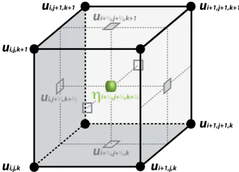
Fig. 1. Grid cell as used in the STAG implementation. Note that velocities are defined at grid points while effective viscosities are computed in the centre. To determine necessary velocity derivatives one first computes the velocity on each face of the grid box.
scheme needs the average of four at each side of the box. Subsequently derivatives are calculated using values at oppo-site faces of the cell, i.e. the derivative inx-direction requires the velocity field averaged in they,ζ-plane. The STAG dis-cretisation of the effective viscosity thereby reduces the trun-cation error of the velocity derivatives with respect to DIR. Note however that the truncation error is not necessarily a good indicator for the accuracy of a discrete solution (Veld-mann and Rinzema, 1992) and in particular not for a non-uniform grid spacing.
The main difference between the two schemes lies in the discretisation of the force balance Eqs. (5, 11). This applies to the finite difference approximation used for the two oper-ators;9. The three additional terms, that show mere first derivatives either in velocities or surface elevation, do not show the structure necessary for,9. Consequently a dis-tinct discretisation is used, which we base on centred differ-ences between the two inline-adjacent grid points (analogous to DIR). The two discretisations thus ultimately differ in the realisation of the two operators,9that are defined via
(s, g,f ) ≡∂s(g·∂sf )=∂sg·∂sf+g·∂s2f 9 (s, t, g,f )≡∂s(g·∂tf )=∂sg·∂tf+g·∂s∂tf
(12) In the DIR scheme, operators are rewritten using the chain rule (right hand side of Eq. 10) and the resultant summands show derivatives that are approximated by centred differ-ences of first order. This DIR discretisation is presented in detail in Pattyn (2003). It accepts that the discretisation of
be determined on the relevant, staggered position for a cen-tred difference approximation of the outer derivative. With the finite differences spanning only one grid cell, the STAG scheme shows naturally a reduced truncation error.
A detailed description of the STAG scheme, giving the full decomposition in finite differences, is provided in Ap-pendix B. In this section a more heuristic description is pre-sented to clarify the fundamental steps. To illustrate them, we focus on the horizontal operator9(x,y,η,u)=∂x η·∂yu
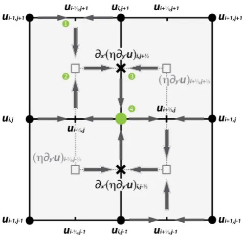
, which has the advantage to act on an equidistant mesh. The term in brackets, still undergoing the derivative inx, is de-termined in between adjacent grid points inx-direction. This allows a central difference approximation of thex-derivative on half the grid spacing. For this purpose both the velocity derivative iny-direction and the effective viscosity need to be determined at the relevant position. As illustrated in Fig. 2, this is achieved in four steps.
1. First, one linearly averages adjacent velocities to get values in between grid points inx-directionu
i+1
2,j . 2. With u
i+1
2,j
, the centred derivative in y-direction is calculated giving(∂yu)
i+1
2,j+ 1 2
in the middle ofx,y -faces. This derivative is then multiplied with a viscos-ity average(η·∂yu)
i+1
2,j+12
of two adjacent grid cell centres.
3. Subsequent computation of the centred derivative in
x-direction of (η ·∂yu) i+1
2,j+ 1 2
provides ∂x(η · ∂yu)
i,j+1
2 .
4. Averaging the derivative field∂x(η ·∂yu) i,j+1
2
linearly in y-direction, one obtains it on the regular grid (cf. Fig. 2).
Swappingx andy, the operator9(y,x,η,u)is determined in an analogue way. Derivatives operating on the vertical axis hold an additional complexity since equal spacing in this direction is not granted. For non-uniform spacing, weight-ing coefficients are used that are based on Newton’s formula for a second-order polynomial approximation (see Eqs. B8 and B9). These two equations can be applied in analogy to the above discussion to determine the STAG version of
9(ζ,x,η,u),9(ζ,y,η,u),9(x,ζ,η,u)and9(y,ζ,η,u).
Foroperators that show two derivatives in the same di-rection, one determines the inner derivative in between ad-jacent grid points with centred differences. This derivative is then multiplied by a four-point average of viscosities that gives(η·∂ u)in between adjacent, in-line grid points. The outer derivative is then determined centred over half the grid spacing. A detailed description of the numerical implemen-tation is presented in Appendix B.
In summary, we have two discretisations of the force bal-ance equation. First the DIR scheme that is based on centred
Fig. 2. Visualization of the operating mode of9(x,y,u,η). In a first step, two adjacent velocities are averaged inx-direction. This field is then used to form the inner derivative iny-direction that is asso-ciated with the grid point staggered in thex,y-plane (step 2). After determining the viscosity in this point, the outerx-derivative can be computed in a third step. The fourth and last step is to average the resultant field inx-direction (a detailed description is presented in Appendix B).
differences for the fully decomposed operators (cf. Pattyn, 2003). As shown, this scheme is not confined to the com-pact stencil for the bulk equation. The STAG discretisation is confined to the compact stencil and makes use of informa-tion on staggered posiinforma-tions. In this way it increases coupling of the velocity solution in adjacent grid points and reduces the truncation error.
2.3 Operator invertibility
In mathematical terms, a structural difference is present in the two ways of discretising the operator. Consider the following ordinary differential equation in one dimension
(x,η,u)=∂x(η ·∂xu)=f, (13)
withf ∈ C(R3). To numerically approximate the solution
we choose a one dimensional grid with uniform spacing1x. The DIR discretisation makes use of the chain rule and ap-proximates the two resulting terms with centred differences. (−ηi−∂xηi1x)·ui+1+(−ηi+∂xηi1x)·ui−1+2ηi·ui= −fi1x2(14)
centred difference approximation for the outer derivative on half the grid extent.
−η
i+12·ui+1−ηi−12·ui−1+
η
i+12+ηi−12
·ui= −fi1x2 (15)
Despite the inherent dependence of the viscosityηon the ve-locity field, we will treat it for now as a given scalar field. Since the viscosity is by definition positive (see Eq. 6), the factors of the diagonal element are positive in both numeri-cal schemes. Both discretisations also result in a matrix M of tridiagonal form. However, the STAG discretisation pro-vides additional structure to M because it guarantees that the off diagonal entries are all negative. In the DIR scheme this is only true as long asηi≥ k1x·∂xηik. The resultant
ma-trix structure for STAG ensures the invertibility of M since an additional requirement holds which states the existence of a vector u with positive components ui>0 that fulfils
(Mu)i>0 (in literature such matrices are referred to as
M-matrices and the interested reader is referred to Berman and Plemmons, 1994). For the DIR scheme, invertibility is not guaranteed especially for large grid spacing or high gradi-ents in the viscosity field. The STAG discretisation will con-sequently stabilise any numerical method that determines the inverse of such a linear system of equations. In other words, the STAG discretisation provides a matrix M that uncondi-tionally inherits a discrete maximum principle from the con-tinuous operator, whereas DIR does so only for sufficiently small mesh sizes.
In addition, if one resolves the velocity dependence of the viscosity for DIR, one notices that theoperator leaves the compact stencil during each non-linear iteration step. This is caused by the appearance of the first viscosity derivative which itself uses centred differences for the velocity gradi-ents. It can give rise to spurious oscillations in the solution, especially in the vicinity of the lateral boundaries. This is also the case for the discretisation of the9 operator. In con-trast to DIR, the STAG discretisation for both operators is al-ways confined to the compact stencil of adjacent grid points.
3 Iterative solver
3.1 Decomposition of the non-linear system of equations
We reduce the complexity of the nonlinear system by de-composing Eq. (11) into coupled linear equations following Pattyn (2003). The key is to iteratively update the effective viscosity that is nonlinearly dependent on the horizontal ve-locity field (see Eq. 6). For each nonlinear iteration step the viscosity field is prescribed. Doing so, the determina-tion of the horizontal velocity field from the force balance Eq. (11) becomes a linear problem. In other words, one pre-scribes an initial velocity field, computes the resulting vis-cosity field and subsequently determines the velocity solu-tion to the force balance. Subsequently one enters the next
nonlinear step and updates the viscosity field that is in turn fed into the linear system.
3.2 Linear iteration
For solving the linear system of equations represented by Eq. (11), another decomposition is made separating the two horizontal components of the velocity vectoruandv. More precisely, knowing both velocity components from the pvious nonlinear iteration, one uses them to retrieve the re-spective perpendicular component in the current iterationr. Thus, the currentru˜becomes a function of both the previous
viscosityr−1ηand the previousy-component of the velocity fieldr−1v. This leads to a numerical decoupling of the x -andy-direction of the force balance equation in the nonlin-ear iterations and consequently reduces the matrix size of the linear system by a factor 4. Using one of the two discretisa-tions of the force balance Eq. (11), one can rewrite them in matrix form assuming the respective perpendicular velocity component as given.
3x(r−1η)ru˜ =Bx(r−1u,r−1v) 3y(r−1η)rv˜ =By(r−1u,r−1v)
(16) The so-called coefficient matrices3are sparse in both dis-cretisations since only a few off-diagonal elements are non-zero. Using a grid of respectively nx, ny,nζ points in the x−,y−andζ-direction, the matrix hasN×N entries with
N=nx·ny·nζ. Among all matrix coefficients, at most 19
out of N are non-zero in each matrix column. This ra-tio falls below one percent for grids consisting of more than 2000 points. Linear systems of equations that show highly sparse matrices are efficiently solved iteratively. One prominent solver for such systems is the bi-conjugate gra-dient (BiCG) method (Press et al., 2003) with a diagonal preconditioner. Iterative methods use in general criteria that define saturated convergence. A build-in criterion is applied that successively computes the ratio of two maximum norms. The numerator shows the precondition matrix applied on the residual while the denominator holds the current correction vector (see Press et al., 2003). A relative toleranceεlin de-fines the stopping criterion for which convergence is reached.
3.3 Non-linear iteration
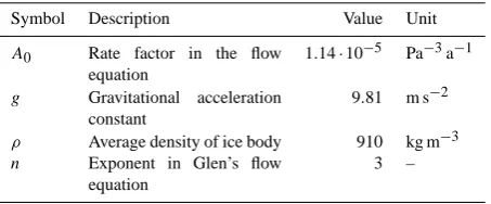
Table 1. Overview of model parameters used in the ISMIP-HOM benchmark (Pattyn et al., 2008).
Symbol Description Value Unit
A0 Rate factor in the flow equation
1.14·10−5 Pa−3a−1
g Gravitational acceleration constant
9.81 m s−2
ρ Average density of ice body 910 kg m−3 n Exponent in Glen’s flow
equation
3 –
information from the previous solution ru =f (ru,˜ r−1u). Although such correction schemes may be beneficial, they perturb a clear comparison of the two numerical schemes and are therefore omitted. Instead, true Picard iterations are used until the ratio of the Euclidean norm of the residual and the norm of the solution between successive iterations falls be-low a certain thresholdεnin. The two criteriaεlin andεnin define the quality of the solution and are referred to as the convergence tolerance or simply the tolerance.
4 Model intercomparison and validation
In the following, results are presented from conducting ex-periments of the ISMIP-HOM model intercomparison study (Pattyn et al., 2008). First the experimental setup is specified that serves to evaluate the two discretisations.
In the framework of this intercomparison study four out of six time independent experiments were selected. The re-maining two add no additional challenge since they are flow-band versions of two others. Test A is a purely geometric problem with an inclined surface topography, frozen bed and sinusoidal bed topography. In test C, a tilted slab of ice with constant thickness is forced with a sinusoidal sliding field
β2 at the base (see Eq. 9). Experiments A and C use peri-odic boundary conditions at the lateral domain margin. In addition, both experiments are conducted for several aspect ratios, i.e. the ratio of ice thickness and domain extent. This ratio is linked to the length scale of the sinusoidal perturba-tions. Test E2 and E1 are applications on the observed geom-etry of Haut Glacier d’Arolla respectively with and without a zone of zero friction. The details to each experimental setup are found in Pattyn et al. (2008) while the suggested model parameters are summarised in Table 1. All experiments were conducted on a grid with 100 equally spaced points in both horizontal directions and 100 exponentially spaced layers in the vertical. For Haut Glacier d’Arolla (exp. E1, E2) the hor-izontal dimension across the flow line was reduced to 83. In all experiments the shallow ice approximation serves to calculate an initial velocity field. The criteria to stop our iterative solver, i.e. the convergence tolerance, are set equal for both linear and non-linear iterationsεnin=εlin=ε.
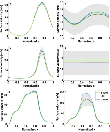
Although the two discretisations yield different solutions to these experiments (Fig. 3), they both reproduce the results of the intercomparison study. Differences become more ev-ident when the aspect ratio decreases (Fig. 3b and c). How-ever, results are in general within the root mean square (rms) deviation of the higher-order model participants of ISMIP-HOM to their average. In the combined geometric and basal boundary problem of test E2, the difference between the STAG and DIR schemes is largest while DIR exceeds the rms deviation, which is large by itself. The fact that solu-tions for E2 show such a high variation is due to the fact that the setup with a zone of no friction might actually be ill posed (see Pattyn et al., 2008). In light of this a direct comparison of the solution is possibly inappropriate. In contrast to some model participants of the E2 experiment, both discretisation schemes suggest smooth solutions suppressing build-up of oscillations where the base supports no resistance. Experi-ments A and C were also conducted on the 20 km domain to check the applicability on intermediate aspect ratios. The resultant velocity fields (not shown) are also in qualitative agreement with the ISMIP-HOM results. Except for exper-iment E2, no major qualitative differences in the solutions are perceived. In Sect. 5.3 non-physical irregularities in the solution are discussed which are observed in experiment A on a 160 km domain.
5 Numerical characteristics
The focus of this section is to compare the two discretisations by concentrating on the characteristics of convergence. First of all, the residual between successive velocity fields during the non-linear iterations is used to validate the quality of the convergence. In a second step the total amount of linear it-erations needed to converge is analysed in both numerical schemes and in a final step, we assess the numerical stability of the discretisation.
5.1 Residual decrease
Fig. 3. Resultant surface velocity fields for the ISMIP-HOM model intercomparison of the DIR and STAG discretisations for experiments A on 160 km (a) and 5 km (b), C on 160 km (c) and 5 km (d) and E1 (e) and E2 (f). The grey shaded area indicates the root mean square (rms) deviation of the solution from each participant compared to the mean benchmark solution (dark grey). For the two discretisations, we chose the solution obtained with the highest possible convergence accuracy (see Table 2). All over the results are in good agreement with the mean of the benchmark test. The only exception is experiment E2 (f) where the DIR velocity field exceeds the wide rms deviation.
5.2 Convergence rate
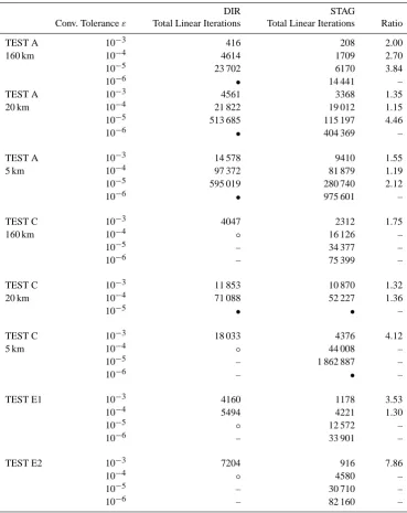
A mere comparison of the iteration accuracy, being deter-mined in the non-linear iteration, does not capture the con-vergence behaviour in the inner, linear iterations. It is the number of linear iterations that holds information about the actually undertaken calculations and thus the computational costs for the convergence (see Table 2). The convergence tol-erance comprises the two thresholdsε=εlin=εninand it is varied in a range from 10−3 to 10−6. Tolerance is defined
Table 2. Convergence behaviour of the DIR and the STAG discretisation for the ISMIP-HOM experiments. The convergence tolerance is equal for linear and non-linear iterations and varied from 10−3to 10−6. Note that the number of linear iterations is proportional to the computational costs. “•” signifies that the accuracy could not be reached and the convergence was manually stopped after an reasonable number of non-linear iterations. Divergence of the resultant velocity field is marked with “◦”. If a certain tolerance was not reached in either way, the same experiment was not conducted with higher accuracy (“–”).
DIR STAG
Conv. Toleranceε Total Linear Iterations Total Linear Iterations Ratio
TEST A 10−3 416 208 2.00
160 km 10−4 4614 1709 2.70
10−5 23 702 6170 3.84
10−6 • 14 441 –
TEST A 10−3 4561 3368 1.35
20 km 10−4 21 822 19 012 1.15
10−5 513 685 115 197 4.46
10−6 • 404 369 –
TEST A 10−3 14 578 9410 1.55
5 km 10−4 97 372 81 879 1.19
10−5 595 019 280 740 2.12
10−6 • 975 601 –
TEST C 10−3 4047 2312 1.75
160 km 10−4 ◦ 16 126 –
10−5 – 34 377 –
10−6 – 75 399 –
TEST C 10−3 11 853 10 870 1.32
20 km 10−4 71 088 52 227 1.36
10−5 • • –
TEST C 10−3 18 033 4376 4.12
5 km 10−4 ◦ 44 008 –
10−5 – 1 862 887 –
10−6 – • –
TEST E1 10−3 4160 1178 3.53
10−4 5494 4221 1.30
10−5 ◦ 12 572 –
10−6 – 33 901 –
TEST E2 10−3 7204 916 7.86
10−4 ◦ 4580 –
10−5 – 30 710 –
10−6 – 82 160 –
only reached for tolerances up to 10−4. Knowing that a toler-ance of at least 10−4is necessary to guarantee saturated con-vergence, this is a grave restriction for the application of the DIR scheme. However, even in cases where the prescribed tolerance could not be reached, we stopped the solver manu-ally after a specific amount of non-linear iterations. This ar-bitrary number was estimated consulting the non-linear steps
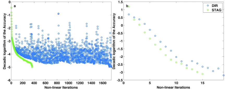
Fig. 4. The residual between successive velocity solutions (i.e. the accuracy) is depicted throughout the non-linear iterations for both discretisations. On the left (a) the convergence of the ISMIP-HOM test A on a 20 km domain is shown. The decrease in DIR is erratic and indicates huge changes in the velocity field even in the last few iteration steps. For the same setup, the STAG scheme is characterised by a more regular decrease in the accuracy until the prescribed tolerance of 10−5is reached. In addition, less non-linear iterations are necessary to retrieve the solution as is confirmed in test C on 20 km (b), where both discretisations show a more regular convergence.
solutions remain in agreement with the ISMIP-HOM results. Anyway a lack in convergence raises concerns about the ap-plicability of the retrieved solution.
5.3 Numerical stability
In all of the conducted ISMIP-HOM intercomparison exper-iments (Pattyn et al., 2008) the STAG scheme gives physi-cally reasonable results, though in two cases not strictly con-verged. But STAG shows robust convergence that prevents possible divergence of the resultant velocity field (see Ta-ble 2 and Fig. 4). Divergence only occurs for the DIR scheme and the retrieved flow field deviates by orders of magnitude from the physically reasonable one. The diverged solution exhibits jagged structures that indicate numerical instability, which occurs preferentially for sliding experiments that ap-ply Neuman boundary conditions at the base. But also for a setup without sliding, DIR diverges as soon as a realistic and rugged geometry is used (compare experiment E1). Di-vergent behaviour is critical since it makes transient experi-ments almost impossible because the velocity solution might destabilise for any realised geometry during the time evolu-tion. To circumvent this problem in DIR, a smoothing algo-rithm was applied on the viscosity field (results not shown). In detail,ηwas linearly interpolated on the centre of the grid box and subsequently interpolated back on the regular grid. This prevented divergence of the resultant velocity field in the DIR scheme. But this smoothing did neither facilitate nor inhibit the convergence process. Moreover, no consistent improvement in the attainable accuracy for the DIR discreti-sation could be stated. For these reasons, such a smoothing algorithm seems capable to prevent divergence but it appears to neither facilitate the convergence rate nor allow for higher
accuracies of the solution. Moreover, solutions from a solver using artificial smoothing are delicate to interpret since they might miss crucial details of the dynamic behaviour.
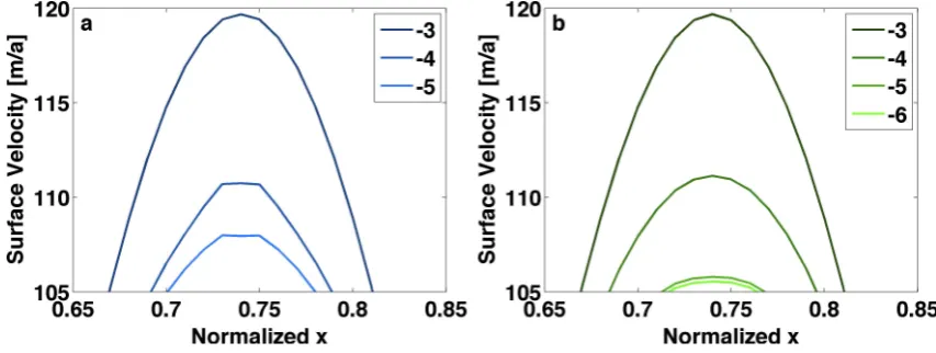
A more detailed examination of the resultant surface ve-locity fields of the ISMIP-HOM test A reveals for coarse resolutions a qualitative difference between the two dis-cretisations. On the 160 km domain, the maximal veloc-ity decreases and seems to saturate with increasing accu-racy (Fig. 5). Remarkable is however a feature appearing in the DIR discretisation. For high tolerances, the maximum becomes locally flat and even shows a local depression for
ε=10−5(see Fig. 5a). This is in contradiction with proper-ties of the solution to the elliptic force balance equations (cf. Eq. 5). For this low aspect ratio, velocities are dominated by vertical plane shearing and magnitudes are comparable with the solution of the shallow ice approximation. In such a situ-ation Appendix C suggets that local extrema in the horizontal velocity field are ultimately linked to extrema in the basal to-pography. A local minimum in bedrock elevation thus goes along with one local maximum in the velocity field. Identi-fying three adjacent local extrema in the DIR velocity field indicates that its discretisation breaks properties of the solu-tion to an elliptic PDE as the force balance Eq. (5). At least, these properties are not captured in this specific example with coarse resolution. Existence of spurious extrema can also be a seed for destabilisation during the iterative process of de-termining the solution.
6 Summary and outlook
Fig. 5. Resultant surface velocity fields in the ISMIP-HOM test A on the largest domain of 160 km for the DIR discretisation (a) and the STAG discretisation (b). This is a close-up view of the zone of high deformation where thex-component of the bedrock gradient changes its sign. The legend entries refer to different convergence tolerances expressed in the exponent of 10. For a low tolerance, both discretisations find a solution close to the initial SIA velocity (not depicted). With increasing accuracy the resultant velocity fields converge to a solution with lower maxima. However, the DIR field levels out at the maxima and even shows a local minimum for the highest accuracy.
ice sheet model. We use a LMLa higher-order model in the notation of Hindmarsh (2004) that applies some simplifica-tion to the full Stokes equasimplifica-tion. The first discretisasimplifica-tion, re-ferred to as the DIR scheme, uses the chain rule to decom-pose all terms in the force balance to substitute each by cen-tred difference, as suggested by Pattyn (2003). The presented new STAG discretisation makes use of the present double derivatives and computes the terms necessary for the outer derivative on staggered grid points (see Fig. 2).
In general both discretisations reproduce the results pre-sented in the ISMIP-HOM model intercomparison study (Pattyn et al., 2008). The good agreement between the two discretisations in the resultant velocity fields encour-ages a clean comparison of their convergence behaviour. Altogether, we note that the new scheme facilitates the con-vergence and reduces the total amount of iterations by a fac-tor of up to 7 and in average 2.6 (see Table 2). This implies a decrease in iterative calculations making STAG computa-tionally more efficient. Another benefit using the new dis-cretisation becomes apparent for increased convergence tol-erance. In most conducted experiments the STAG solution can attain a higher accuracy than possible in the DIR dis-cretisation. This indicates that erratic build-up of oscillations between successive velocity fields is prevented. Spurious os-cillations entering the periodic boundary conditions will even more deteriorate the solution of the linear part of the solver and inhibit convergence for high tolerance. The attainable higher tolerance for the STAG solution therefore indicates more robust numerics. For experiment A on the coarsest resolution, the DIR surface velocity field along a flow line shows three adjacent local extrema in the zone of fastest flow. For this experiment, such features are per se not feasible in the solution to the elliptic, partial differential equation for the force balance. Additionally, such local irregularities can be a
seed for destabilisation of the iterative process. In four out of 18 experiments destabilisation even causes divergence of the DIR velocity field throughout the iterations. Consequently no physical velocity solution is found for a specific experi-mental setup. Such deficiency is not observed in the STAG scheme indicating robustness of its numerical discretisation, which prevents the iterative build up of perturbations.
Increased convergence rate, higher accuracy and preven-tion of divergence in the STAG discretisapreven-tion make the pre-sented discretisation more reliable for any application on ob-served or artificial geometries. Especially in time-dependent mode, with prognostic evolution of the ice geometry, diver-gence in the velocity solution would pose a huge problem. Being more robust the new discretisation stabilises the tran-sient behaviour. But not only a converged velocity field is im-portant in time dependency. Also accuracy is decisive since low accuracy results in not fully converged velocity fields and consequently an inadequate geometry evolution. These inaccuracies in turn feed back on the velocity field of the next time step and thus transmit in a prognostic way. Only high accuracy guarantees physically correct feedbacks between higher order dynamics and geometry evolution in transient applications.
minimal residual method (GMRES in Saad and Schultz, 1986), multigrid approaches (see Wesseling and Sonneveld, 1980; Trottenberg et al., 2001), the induced dimension re-duction (IDR) method (Sonneveld and van Gijzen, 2008; van Gijzen and Sonneveld, 2011) or a combination of IDR and BiCGstab called IDRstab (Sleijpen and van Gijzen, 2010). In line with replacing the solver is the use of a more appropriate preconditioner for matrix inversion for incompressible fluid dynamics (see Manguoglu et al., 2009). Another option is to combine the applied solver with some correction algorithm that improves the convergence rate. A useful relaxed Picard iteration was presented in De Smedt et al. (2010). An addi-tional improvement to the presented discretisation could be expected by a strict separation of geometry on regular points and velocity on staggered points as suggested by Harlow and Welch (1965). More recently Hyman et al. (2002) suggest a mimetic finite difference method for diffusion problems (as theoperator) that satisfies conservation laws and is appli-cable for nonsmooth and unstructured grids. In case Neu-mann boundary conditions are used at the base, a revision of the centred discretisation of the boundary layer equation may give additional numerical benefits.
Appendix A
A dimensionless vertical coordinate system is used that nor-malises the vertical axis viaζ =(s−z)/H. This results in a vertical coordinate that varies from zero at the surfacesto one at the glacier bedb. Since the two horizontal axes remain unchanged, the Jacobian of this coordinate transformation to
(x0, y0, ζ )takes a simple form (also compare Pattyn, 2003). For a functionf =f (x,y,z)in the class ofktimes contin-uous differentiable functionsCk(R3)(fork≥2) this yields
∂xf =∂x0f +ax·∂ζf
∂yf =∂y0f +ay·∂ζf
∂zf =az·∂ζf,
(A1)
while the coefficients denote the non-zero elements of the Jacobian.
ax =∂x0ζ= 1
H(∂x0s−ζ ·∂x0H ) ay =∂y0ζ= 1
H(∂y0s−ζ ·∂y0H ) az =∂zζ = −H1
(A2)
However, the balance Eq. (5) also shows second order derivatives in all variables. Only four of the possible second derivates actually occur.
∂xxf =∂x0x0f +bx·∂ζf +a2
x·∂ζ ζf +2ax·∂x0ζf
∂yyf =∂y0y0f +by·∂ζf +a2
y·∂ζ ζf +2ay ·∂y0ζf
∂zzf =a2z ·∂ζ ζf
∂xyf =∂x0y0f +cxy·∂ζf +ay·∂x0ζf +ay·∂y0ζf+
axay ·∂ζ ζf,
(A3)
For these derivatives the coefficients are defined as follows
bx =∂x0ax +ax·∂ζax
by =∂y0ay +ay·∂ζay
cxy=∂x0ay +ax·∂ζay.
(A4)
Appendix B Discretisation of bulk equation
This section deals with the detailed description of the nu-merical discretisation of the bulk Eq. (11). In the following a short overview is given how the two operators, 9 are numerically realised for an equidistant mesh as well as for a non-equidistant mesh with weighting based on Newton’s parabolic interpolation formula.
B1 Equidistant mesh
In the horizontal plane the adjacent grid points have uniform spacing (1x, 1y). Thus horizontal derivatives can directly be translated via centred differences. It is sufficient to present the operators(x,η,u)and9(y,x,η,u)since the other two horizontal operators follow in analogy.
B1.1 In-line derivative(x,η,u)
The in-line derivative (x,η,u) is formed by determining the inner termη·∂xuin the centre between to adjacent points
inx. These are subsequently used to determine the outer centred derivative. In detail this reads.
ηi+1/2,j ∂u∂x
i+1 2,j
= 1
21x
h
ui+1,j−ui,j
·ηi+1 2,j+
1 2
+ηi+1 2,j−
1 2
i
ηi−1/2,j ∂u∂x
i−1 2,j
= 1
21x
h
ui,j−ui−1,j
·
ηi−1 2,j+12
+ηi−1 2,j−12
i (B1)
In the vertical both terms are determined on grid layers (index omitted) and, since viscosities are defined in grid box centres, one has to average on layerξk.
ηi+1 2,j+
1 2
= ζk−ζk−1
ζk+1−ζk−1 ·ηi+1
2,j+ 1 2,k+
1 2
+
ζk+1−ζk ζk+1−ζk−1
·ηi+1 2,j+
1 2,k−
1
2 (B2)
Knowing the inner derivative in between adjacent points inx-direction, the outerx-derivative of(x,η,u)is conve-niently approximated by a centred difference.
∂ ∂x
η ∂u∂x
i,j=
1
1x
h
ηi+1 2,j
∂u ∂x
i+12,j−ηi−11 2,j
∂u ∂x
i−12,j
i
=
= 1
21x2
h
ui+1,j
ηi+1 2,j+
1 2
+ηi+1 2,j−
1 2
+
ui−1,j
ηi−1 2,j+
1 2
+ηi−1 2,j−
1 2
−
ui,j
ηi+1 2,j+12
+ηi+1 2,j−12
+ηi−1 2,j+12
+ηi−1 2,j−12
i
(B3)
B1.2 Cross derivative9(y,x,η,u)
y-direction. A centred derivative inx of this averaged ve-locity field defines(∂xu)i+1
2,j+ 1 2
, staggered in thex− and
y-direction. As before, the effective viscosity is vertically averaged to findηi+1
2,j+ 1 2
(cf. Eq. B2).
ηi−1 2,j+
1 2
∂u ∂x
i−1
2,j+ 1 2
= 1 21xηi−1
2,j+ 1 2 ·
ui,j+1+ui,j− ui−1,j+1+ui−1,j ηi−1
2,j− 1 2
∂u ∂x
i−12,j−12=
1 21xηi−1
2,j− 1 2 ·
ui,j+ui,j−1− ui−1,j+ui−1,j−1 (B4)
These two terms are averaged inx-direction after they -derivatives are determined via centred differences.
∂ ∂y
η ∂u∂x
i,j= 1 2 ∂ ∂y n
η ∂u∂x
i−12,j+12+
η ∂u∂x
i+12,j+12
o = = 1 41y1x h ui,j
ηi−1 2,j+
1 2
+ηi+1 2,j−1
1 2
−
ηi−1 2,j−
1 2
ηi+1 2,j+
1 2
+
ui,j+1
ηi−1 2,j+
1 2
−ηi+1 2,j+
1 2
+
ui,j−1
ηi+1 2,j−
1 2
−ηi−1 2,j−
1 2
+
ui+1,j
ηi+1 2,j+
1 2
−ηi+1 2,j−
1 2
+
ui−1,j
ηi−1 2,j−
1 2
−ηi−1 2,j+
1 2
+
ui−1,j−1ηi−1 2,j−
1 2
+ui+1,j+1ηi+1 2,j+
1 2
−
ui+1,j−1ηi+1 2,j−
1 2
−ui−1,j+1ηi−1 2,j+
1 2
i
(B5)
Given these two examples, forms (y,η,u) and
9(x,y,η,u)follow by simple substitution.
B2 Vertically non-equidistant mesh
With a generally non-equally spaced vertical grid, a finite dif-ference scheme for the two operators becomes more elabo-rate. First we introduce some notation for the chosen vertical spacingξk.
1ζ k+1
2
=ζk+1−ζk or1ζk = 12(ζk+1−ζk−1) (B6) In the vertical the Newton formula yields the following interpolation for a second order approximation of function valuesfk.
fk= 1ζ
k+1
2 2·1ζk
·fk−1 2
+
1ζ k−1
2 2·1ζk
·fk+1
2 (B7)
This weighting can be used to retrieve a finite difference approximation for the vertical derivative based on a centred scheme. ∂f ∂ζ k = 1ζ k−1
2
1ζ k+1
2 ·1ζk
·f k+1
2 −
1ζ k+1
2
1ζ k−1
2 ·1ζk·f
k−1
2 +
1ζ k+1
2 −1ζ
k−1
2
1ζ k+1
2 ·1ζ
k−1
2
·fk (B8)
Assuming equal vertical spacing (1ζk =1ζ k+1
2 =
1ζ k−1
2
=1ζ )this form reduces to the normal centred dif-ference approximation by removing the last term.
B2.1 In-line derivative(ξ,η,u)
In analogy to the equally spaced grid but applying Eqs. (B6)– (B8), this in-line derivative is computed as follows. For the in-line staggered point, the inner derivatives can directly be calculated using centred differences. However, the termη∂ξu
will also be needed on the regular grid and for this we use Eq. (B8).
ηi,j,k+1 2
·∂u
∂ζ
i,j,k+12
= 1
1ζ
k+1
2
ηi,j,k+1 2
·ui,j,k+1−ui,j,k
ηi,j,k· ∂u ∂ζ i,j,k =1 2ηi,j,k·
( 1ζ
k−1
2
1ζ
k+1
2
1ζkui,j,k+1 −
1ζ
k+1
2
1ζ
k−1
2
1ζk ui,j,k−1+
1ζ
k+1
2
−1ζ
k−1
2
1ζ
k+1
2
1ζ
k−1
2
ui,j,k )
ηi,j,k−1 2
·∂u
∂ζ
i,j,k−12
= 1
1ζ
k−1
2
ηi,j,k−1 2
·
ui,j,k−ui,j,k−1 (B9)
Since effective viscosities are needed on respective inter-mediate grid points, one averages the calculated staggered values ηi+1
2,j+ 1 2,k+
1
2 appropriately. The extra division by two appearing in the expression forηi,j,k· ∂ζui,j,k,
origi-nates from determining the three terms in Eq. (B8) on the regular grid. Applying the same equation another time, now unmodified, one obtains a numerical approximation for
(ζ,η,u).
∂ ∂ζ
η∂u∂ζ
i,j,k
=
1ζ
k−1 2 21ζ2
k+1 2
1ζk
ηi,j,k+1 2
·∂u
∂ζ
i,j,k+1
2 −
1ζ
k+1
2 21ζ2
k−1
2
1ζk
ηi,j,k−1 2
·∂u
∂ζ
i,j,k−12
+
1ζ
k+1
2
−1ζ
k−1
2
!
21ζ
k+1
2
1ζ
k−1
2
ηi,j,k·
∂u ∂ζ
i,j,k
= ui,j,k+1·
1ζ
k−1
2 21ζ2
k+1
2
1ζk
ηi,j,k+1 2
+
1ζ
k+1
2
−1ζ
k−1
2
!
21ζ2 k+1
2 1ζk ηi,j,k +
ui,j,k−1·
1ζ
k+1
2 21ζ2
k−1
2
1ζk
ηi,j,k−1 2
+
1ζ
k+1
2
−1ζ
k−1
2
!
21ζ2 k−1
ui,j,k · 1ζ
k+1
2
−1ζ
k−1
2
!2
21ζ2
k+1
2
1ζ2
k−1
2
ηi,j,k−
1ζ
k+1
2 21ζ2
k−1
2
1ζkηi,j,k− 1 2
−
1ζ
k−1
2 21ζ2
k+1
2
1ζkηi,j,k+ 1 2
Again, assuming uniform spacing in the vertical, this equa-tion reduces to the form(x,η,u)in Eq. (B3).
B2.2 Cross derivative9(x,ξ,η,u)
This function’s inner derivative is computed with a centred difference scheme. But in analogy to the equidistant form, the velocities are beforehand averaged inx-direction. This provides values for∂x(η·∂ζu)i+12,j,k+12 at each centre of grid
box x,ζ-faces.
η
i−1 2,j,k+
1 2 ∂u ∂ζ
i−1 2,j,k+
1 2
= 1
21ζ
k+1 2
η
i−1 2,j,k
+
1 2·
ui,j,k+1−ui,j,k
+ ui−1,j,k+1−ui−1,j,k (B11)
To compute the final derivative on the regular grid (cf. Fig. 1), vertical averaging becomes necessary followed by approximating the horizontal derivative by a centred differ-ence. ∂ ∂x η ∂u ∂ζ i,j,l= 1 41x 1ζk
ui+1,j,k−1·
−
1ζk+1 2 1ζk−1 2
ηi+1 2,j,k−
1 2
+
ui−1,j,k−1·
1ζ k+1
2 1ζ
k−1 2
ηi−1 2,j,k−
1 2
+
ui+1,j,k+1·
1ζ
k−1 2 1ζ
k+1 2
ηi+1 2,j,k+
1 2
+
ui−1,j,k+1·
−
1ζ k+1
2 1ζk−1 2
ηi−1 2,j,k+
1 2
+
ui+1,j,k·
1ζ k+1
2 1ζ
k−1 2
ηi+1 2,j,k−12
−
1ζ k−1
2 1ζ
k+1 2
ηi+1 2,j,k+12
+
ui−1,j,k·
−
1ζk+1 2 1ζ
k−1 2
ηi−1 2,j,k−
1 2
+
1ζk−1 2 1ζ
k+1 2
ηi−1 2,j,k+
1 2
+
ui,j,k+1·
1ζ k−1
2 1ζk+1 2
ηi+1 2,j,k+
1 2
−
1ζ k+1
2 1ζk−1 2
ηi−1 2,j,k+
1 2
+
ui,j,k−1·
−
1ζk+1 2 1ζ
k−1 2
ηi+1 2,j,k−12
+
1ζk+1 2 1ζ
k−1 2
ηi−1 2,j,k−12
+
ui,j,k·
1ζ k+1
2 1ζk−1 2
ηi+1 2,j,k−
1 2
−
1ζ k+1
2 1ζk−1 2
ηi−1 2,j,k−
1 2
+
1ζ k−1
2 1ζ
k+1 2
ηi−1 2,j,k+
1 2
−
1ζ k−1
2 1ζ
k+1 2
ηi+1 2,j,k+
1 2
(B12)
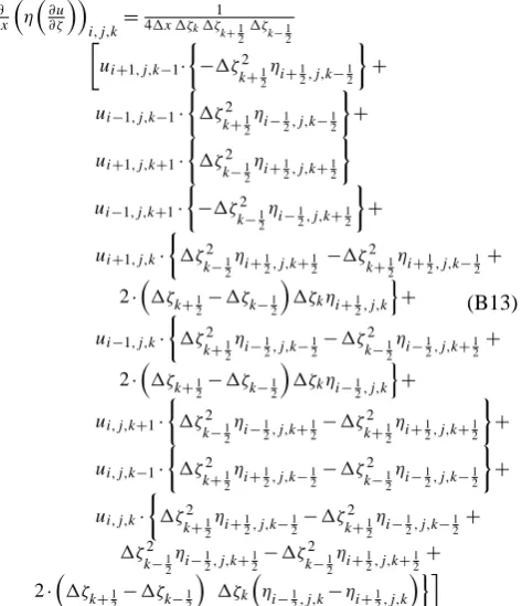
B2.3 Cross derivative9(ζ,x,η,u)
Swapping the sequence of derivatives affects the numerical realisation of 9(ζ,x,η,u) for the non-equidistant vertical spacing. This means one cannot just swap the indices in Eq. (B12) to retrieve the respective coefficients. Anyway,
the derivation is in analogy to the previous operator (see also Fig. 1) and one finds the following approximation.
∂ ∂x
η∂u∂ζ
i,j,k
= 1
41x 1ζk1ζk+1 2
1ζ k−1
2
ui+1,j,k−1·
−1ζ2
k+12ηi+12,j,k−12
+
ui−1,j,k−1·
1ζ2
k+12ηi−12,j,k−12
+
ui+1,j,k+1·
1ζ2
k−1 2
ηi+1 2,j,k+
1 2
ui−1,j,k+1·
−1ζ2
k−12ηi−12,j,k+ 1 2
+
ui+1,j,k·
1ζ2
k−12ηi+12,j,k+12 −1ζ
2
k+12ηi+12,j,k−12+
2·
1ζk+1 2
−1ζk−1 2
1ζkηi+12,j,k
o +
ui−1,j,k·
1ζ2
k+12ηi−12,j,k− 1 2
−1ζ2
k−12ηi−12,j,k+ 1 2
+
2·1ζk+1 2
−1ζk−1 2
1ζkηi−12,j,k
o +
ui,j,k+1·
1ζ2
k−12ηi−12,j,k+12−1ζ
2
k+12ηi+12,j,k+12
+
ui,j,k−1·
1ζ2
k+12ηi+12,j,k−12−1ζ
2
k−12ηi−12,j,k−12
+
ui,j,k·
1ζ2
k+12ηi+12,j,k− 1 2
−1ζ2
k+12ηi−12,j,k− 1 2
+
1ζ2
k−12ηi−12,j,k+12−1ζ
2
k−12ηi+12,j,k+12+
2·1ζk+1 2
−1ζk−1 2
1ζk
ηi−1 2,j,k
−ηi+1 2,j,k
oi
(B13)
Since the vertical derivative is computed with vertical weighting (see Eq. B8), terms showing differences in ad-jacent layers thicknesses1ζk+1/2−1ζk−1/2 appear in this equation. These terms are highly sensitive to the actual struc-ture of the used vertical discretisation. Note that the two cross derivatives 9(ζ,x,η,u) and9(x,ζ,η,u)are numeri-cally not the same.
Appendix C Analysis on large scales
In this section an argument is derived for local extrema in the velocity field of the higher-order model on large-scale ice sheets. Extrema in the surface velocity field are ultimately linked to extrema in bedrock topography.
For the following analysis, the force balance Eq. (11) is reduced to 2 dimension. This allows rewriting the elliptic operator
P[u(x,ζ )]=f (x) (C1)
with
P[u(x,ζ )]=4·(x,η,u)+4ax· {9(x,ζ,η,u)+ 9(ζ,x,η,u)} + 4ax2+az2·(ζ,η,u) f (x)=ρg·∂xs
(C2)
As surface boundary condition serves a reduced form of Eq. (7)
4 ∂x0u+ax·∂ζu·∂x0s+
1
Since a large-scale ice sheet is considered where the length scale of perturbations is long compared to the ice thickness (as in experiment A on 160 km), the following assumptions are made. At first the effective viscosity is assumed to be a constantη(x,ζ )=η0, which simplifies the double mixed derivatives in the two operators.
P[u(x,ζ )]≈4η0·∂x2u+8axη0·∂xζ2 u+
4ax2+a2zη0·∂ζ2u (C4) This equation illustrates the elliptic character of the un-derlying partial differential equation. Ellipticity signifies an inequality for the three factors, which is here automatically fulfilled.
4η0·
4ax2+a2zη0−14(8axη0)2=4η20a2z>0 (C5)
The second assumption for large-scale ice sheets is that vertical plane shearing is well described by the shallow ice approximation. This links vertical velocity gradients to the surface slope.
∂ζu≈2A0(ρg)nHn+1ζn· |∂xs|n−1∂xs (C6)
With these assumptions we focus on the near surface re-gion, i.e.ζ=ε1. The second vertical derivative and the coefficientaxbecome.
∂ζ2u|ε≈2A0(ρg)nHn+1nεn−1· |∂xs|n−1∂xs ax|ε =H1(∂xs−ε·∂xH )=
1
H((1−ε)·∂xs−ε·∂xb)
(C7) Near the surface the upper boundary condition (C3) is ap-plicable, linking vertical and horizontal derivatives. Together with Eqs. (C7) the operator takes the following form.
P[u(x,ζ )]≈n4η0
H ((1−ε)·∂xs−ε·∂xb)− η0 H·∂xs
o ·∂xζ2 u+
2nA0η0(ρg)n 4ax2+az2
Hn+1εn−1· |∂xs|n−1∂xs
(C8) For a constitutive equation using a flow index of three, terms with exponents higher than 1 inεare neglected. This finally provides
P[u(x,ζ )]≈η0
H
4(1−ε)·∂xs+4ε·∂xb−
1
∂xs
·∂xζ2 u
=ρg·∂xs (C9)
With the assumption that the vertical part of the double derivative is well described by the shallow shelf approxima-tion, this derivative does not change sign. Thus changes in signs due to the bedrock topography have to be compensated for by the horizontal velocity derivative as long as the right hand side and thus the surface slope does not change sign.
Applied to the main flow line in experiment A of the ISMIP-HOM model intercomparison (Pattyn et al., 2008) on a 160 km domain, the surface slope is a constant value, while ice thickness varies sinusoidal together with bedrock topog-raphy. Thus all terms of the sum are constant except for the bedrock topography. Where the ice depth is deepest, the bed slope changes from negative to positive sign causing thex -velocity gradient to change likewise in a close vicinity. This
results in a maximal velocity since the vertical derivative part is supposed to show a negative sign. Consequently in this case of low aspect ratio, velocity extrema are ultimately linked to bed topography.
Acknowledgements. The research was funded mainly by the Com-mission of the European Communities through the Marie Curie Re-search Training Networks program Network of Ice sheet and Cli-mate Evolution (NICE) under contract number MRTN-CT-2006-036127, by the Research Foundation – Flanders (FWO) project NEEM-B on Nested modelling of the Greenland ice sheet in sup-port of the dating and the interpretation of the NEEM ice core record. This work was also supported by funding from the ice2sea programme from the European Union 7th Framework Programme, grant number 226375. Ice2sea contribution number 053. We want to also express our gratitude to the reviewers Torsten Albrecht, Frank Pattyn but especially to Jed Brown whose review comments improved the clarity and quality of the presented work.
Let me again express my thanks for your commitment and the considerable work you have done.
Edited by: C. Ritz
References
Albrecht, T., Martin, M., Haseloff, M., Winkelmann, R., and Lever-mann, A.: Parameterization for subgrid-scale motion of ice-shelf calving fronts, The Cryosphere, 5, 35–44, doi:10.5194/tc-5-35-2011, 2011.
Benn, D. I., Warren, C. R., and Mottram, R. H.: Calving processes and the dynamics of calving glaciers, Earth-Sci. Rev., 82, 143– 179, doi:10.1016/j.earscirev.2007.02.002, 2007.
Berman, A. and Plemmons, R. J.: Nonnegative Matrices in the Mathematical Sciences, Society for Industrial and Applied Math-ematics (SIAM), ISBN:978-0898713213, 1994.
Blatter, H.: Velocity and stress fields in grounded glaciers: a simple algorithm for including deviatoric stress gradients, J. Glaciol., 41, 333–344, 1995.
Bueler, E. and Brown, J.: Shallow shelf approximation as a “sliding law” in a thermomechanically coupled ice sheet model, J. Geophys. Res.-Earth, 114(F03008), 21 pp., doi:10.1029/2008JF001179, 2009.
Colinge, J. and Blatter, H.: Stress and velocity fields in glaciers: Part I. Finite-difference schemes for higher-order glacier models, J. Glaciol., 44), 448–456, 1998.
De Smedt, B., Pattyn F., and De Groen, P.: Using the unstable manifold correction in a Picard iteration to solve the velocity field in higher-order ice-flow models, J. Glaciol., 56, 257–261, doi:10.3189/002214310791968395, 2010.
Dukowicz, J. K., Price, S. F., and Lipscomb, W. H.: Consistent approximations and boundary conditions for ice-sheet dynam-ics from a principle of least action, J. Glaciol., 56, 480–496, doi:10.3189/002214310792447851, 2010.
Ferziger, J. H. and Peri´c, M.: Computational Methods for Fluid Dynamics, Springer Verlag, 3, ISBN:978-3540594345, 2002. Fowler, A. C. and Larson, D. A.: The uniqueness of steady state