Automatic generation of large ensembles for air quality forecasting using the Polyphemus system

(1)

Geosci. Model Dev., 3, 69–85, 2010 www.geosci-model-dev.net/3/69/2010/

Geoscientific

Model Development

Automatic generation of large ensembles for air quality forecasting

using the Polyphemus system

D. Garaud1,2and V. Mallet2,1

1_{CEREA, joint research laboratory ENPC – EDF R&D, Universit´e Paris-Est, Marne-La-Vall´ee, France} 2_{INRIA, Rocquencourt, France}

Received: 19 June 2009 – Published in Geosci. Model Dev. Discuss.: 9 July 2009

Revised: 15 December 2009 – Accepted: 18 December 2009 – Published: 18 January 2010

Abstract. This paper describes a method to automatically generate a large ensemble of air quality simulations. Such an ensemble may be useful for quantifying uncertainty, im-proving forecasts, evaluating risks, identifying process weak-nesses, etc. The objective is to take into account all sources of uncertainty: input data, physical formulation and nu-merical formulation. The leading idea is to build different chemistry-transport models in the same framework, so that the ensemble generation can be fully controlled. Large en-sembles can be generated with a Monte Carlo simulations that address at the same time the uncertainties in the input data and in the model formulation. This is achieved using the Polyphemus system, which is flexible enough to build various different models. The system offers a wide range of options in the construction of a model: many physical parameterizations, several numerical schemes and different input data can be combined. In addition, input data can be perturbed. In this paper, some 30 alternatives are available for the generation of a model. For each alternative, the op-tions are given a probability, based on how reliable they are supposed to be. Each model of the ensemble is defined by randomly selecting one option per alternative. In order to decrease the computational load, as many computations as possible are shared by the models of the ensemble. As an example, an ensemble of 101 photochemical models is gen-erated and run for the year 2001 over Europe. The models’ performance is quickly reviewed, and the ensemble structure is analyzed. We found a strong diversity in the results of the models and a wide spread of the ensemble. It is notewor-thy that many models turn out to be the best model in some regions and some dates.

Correspondence to: D. Garaud

([email protected])

1 Introduction

Due to the great uncertainties that arise in air quality model-ing, ensembles of simulations are now considered in a wide range of applications. They are primarily built for uncer-tainty estimation. They can therefore evaluate the reliabil-ity of exposure studies based on model simulations. In the context of short-term forecasts, they can be used to eval-uate risks, with probabilistic forecasts (e.g., threshold ex-ceedence). Uncertainty estimation may also be useful for screening studies in which the impact of emission abatement, as predicted by numerical simulations, should be compared with the uncertainties. Data assimilation is another appli-cation where ensembles are often used: e.g., in the popu-lar ensemble Kalman filter, the background-error covariance matrix is derived from them. For operational forecasts, an ensemble simulation may be sequentially aggregated so as to form forecasts better than the individual models.

A key step is the generation of the ensembles. They may be built (1) with perturbations in the input data to a single model or with an ensemble of input data (Straume, 2001), (2) with models that share little or no computer code (Gal-marini et al., 2004; McKeen et al., 2005), or with models built on the same modeling platform. Uncertainty estima-tion, for instance, has been conducted with Monte Carlo sim-ulations, thus with perturbations in the input data to a given model (Hanna et al., 1998; Beekmann and Derognat, 2003), and with different models built on the same platform (Mal-let and Sportisse, 2006b). In data assimilation, the ensem-ble Kalman filter (Evensen, 1994) approximates background-error covariance matrices using an ensemble of simulations generated with perturbations in the input data (in air quality, e.g., Segers, 2002). A few studies make use of ensembles composed of models developed in different teams (for long-term simulations, see van Loon et al., 2007). For operational

(2)

forecasting, a weighted linear combination of models can form an improved forecast, as has been shown with an en-semble of models from different teams (Pagowski et al., 2006) and with an ensemble built on the same modeling plat-form (Mallet and Sportisse, 2006a; Mallet et al., 2009).

Whatever the application may be, a key step is the genera-tion of the ensemble. In an ideal setting, one should take into account all uncertainty sources based on the best description available. Essentially, this would mean relying on Monte Carlo perturbations for uncertain input data like emissions, on the alternative descriptions available for data like land use cover, on calibrated ensemble weather forecasts, on dif-ferent formulations for the subgrid parameterizations in the chemistry-transport models, on different numerical schemes in the chemistry-transport models. In this paper, we tend to this ideal setting with a simplified approach: we do not use a meteorological ensemble (the meteorological inputs are treated like other input data), and we rely on an alternative sampling approach to full Monte Carlo simulations. Never-theless all uncertainty sources can be considered, and they are all taken into account at the numerical-simulation stage: no statistical correction is applied in a postprocessing. The approach described in this paper may be seen as a three-fold extension that of Mallet and Sportisse (2006b): new uncer-tainty sources are included, the unceruncer-tainty in input data is specifically taken into account, and the ensemble generation is entirely automatic.

From a technical point of view, building an ensem-ble of simulations is rather straightforward in the case of Monte Carlo simulations: one simply applies random turbations to the input data of a single model. The per-turbation scheme may be complex if it takes into account spatial and temporal correlations in the input fields and if advanced Monte Carlo variants are implemented. However this involves little complexity compared to building an en-semble composed of different models, e.g. of models based on various chemical mechanisms. There are essentially two ways (that may be combined) to form an ensemble with dif-ferent models. One is to use existing models, usually de-veloped in research groups. The resulting ensemble then includes a small number of models, say about ten. An-other way is to generate different models within the same modeling platform: the models are assembled using basic components such as the chemical mechanism or the depo-sition module. Building such a platform is a tedious task, but it makes the generation of ensembles, even very large ones, practicable. In addition, the structure of the ensemble is fully controlled, which eases the scientific interpretation. This approach has been implemented in the modeling sys-tem Polyphemus (Mallet et al., 2007b), and it is described in this paper.

All the models considered in the platform assume that the concentrations of pollutants satisfy a system of partial dif-ferential equations and they approximate their solutions by discretizing the equations in an Eulerian framework. Each

equation of the system is an advection–diffusion–reaction equation of the form:

∂ci

∂t = −div(Vci)+div

ρK∇ci ρ

+χi(c,t )+Ei−3ci,(1) where ci is the concentration of the ith species, c=

(c1,...,cS)is the vector of all concentrations, V the wind vector, K is the turbulent diffusion matrix,ρthe air density, χi the production term due to chemical reactions involving speciesi,Ei represents the emissions and3ci accounts for losses due to scavenging. The boundary conditions at ground level involve the surface emissionsSi and the deposition ve-locityvi:

K∇ci·n=Si−vici, (2)

ifnis the upward-oriented normal to the ground.

All models solve a system of reactive transport equations like Eq. (1), but they rely on different coefficients in the equations (e.g., in the chemistryχi) and on different numer-ical schemes. The coefficients in the equations are estimated according to data from many sources (emission inventory, meteorological model, etc.) and many physical parameteri-zations (vertical diffusion, photolysis attenuation, etc.). We therefore uniquely define a model with (1) the input data and the physical parameterizations it uses and (2) its numerical schemes. Many alternative parameterizations, data sources and numerical schemes are available in Polyphemus – this flexibility is part of Polyphemus design principles. Most op-tions are described in Sect. 2 which identifies the models that can be built on the platform.

In Sect. 3, the actual generation of the ensemble is ad-dressed. This means selecting the models, also called en-semble members, which in turn means selecting the compo-nents (input data, physical parameterization, numerical op-tions) for every model. One model is actually a set of pro-grams that are launched in a given order. The simulation chain should be properly established to take into account the dependencies (e.g., the deposition velocities depend on the land use cover). It should also share the common tions among groups of models and distribute the computa-tions over several computer processors in order to minimize the overall computational time. In addition to the changes in the physical and numerical formulations, several input fields that appear in the reactive transport equation are perturbed. It is assumed that the fields have a normal or a log-normal distribution, and they are perturbed accordingly.

In Sect. 4, the method is illustrated with a 101-member ensemble with gas-phase chemistry only.

2 Building one model

(3)

D. Garaud and V. Mallet: Ensemble generation 71

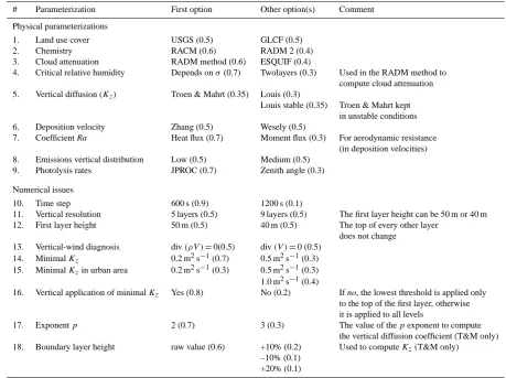
Table 1. Alternatives for the physical parameterizations and numerical options. The numbers enclosed in brackets correspond to the

occurrence probability of an option.

# Parameterization First option Other option(s) Comment

Physical parameterizations

1. Land use cover USGS (0.5) GLCF (0.5)

2. Chemistry RACM (0.6) RADM 2 (0.4)

3. Cloud attenuation RADM method (0.6) ESQUIF (0.4)

4. Critical relative humidity Depends onσ(0.7) Twolayers (0.3) Used in the RADM method to compute cloud attenuation 5. Vertical diffusion (Kz) Troen & Mahrt (0.35) Louis (0.3)

Louis stable (0.35) Troen & Mahrt kept in unstable conditions 6. Deposition velocity Zhang (0.5) Wesely (0.5)

7. Coefficient Ra Heat flux (0.7) Moment flux (0.3) For aerodynamic resistance (in deposition velocities) 8. Emissions vertical distribution Low (0.5) Medium (0.5)

9. Photolysis rates JPROC (0.7) Zenith angle (0.3)

Numerical issues

10. Time step 600 s (0.9) 1200 s (0.1)

11. Vertical resolution 5 layers (0.5) 9 layers (0.5) The first layer height can be 50 m or 40 m 12. First layer height 50 m (0.5) 40 m (0.5) The top of every other layer

does not change 13. Vertical-wind diagnosis div(ρV )=0(0.5) div(V )=0 (0.5)

14. MinimalKz 0.2 m2s−1(0.7) 0.5 m2s−1(0.3) 15. MinimalKzin urban area 0.2 m2s−1(0.3) 0.5 m2s−1(0.3) 1.0 m2s−1(0.4)

16. Vertical application of minimalKz Yes (0.8) No (0.2) If no, the lowest threshold is applied only to the top of the first layer, otherwise it is applied to all levels

17. Exponentp 2 (0.7) 3 (0.3) The value of thepexponent to compute

the vertical diffusion coefficient (T&M only) 18. Boundary layer height raw value (0.6) +10% (0.2) Used to computeKz(T&M only)

–10% (0.1) +20% (0.1)

2.1 Physical formulation (parameterizations and input data)

2.1.1 Land use cover

The land use cover (LUC) describes the material covering the ground with a few categories. Polyphemus supports the USGS (U.S. Geological Survey) LUC with its 24 categories and the GLCF (Global Land Cover Facility) LUC that in-cludes 14 categories. Both LUC have a 1×1 km2resolution, with categories such as grassland, cropland, deciduous for-est, urban areas, etc.

2.1.2 Chemistry

The chemical mechanism is a simplified representation of at-mospheric chemistry, here related to photochemical activity. The mechanism includes species that may or may not exist as such, since many (real) chemical species are lumped into a few (model) species (e.g., the terminal alkenes are lumped into “OLT” in RACM). The mechanism describes the

chem-ical reactions between these species. Here, we consider two chemical mechanisms: RADM 2 (Stockwell et al., 1990) with 61 species and 157 reactions, and RACM (Stockwell et al., 1997) with 72 species and 237 reactions.

2.1.3 Critical relative humidity

The critical relative humidity is used to compute the cloud fraction, the cloudiness and the attenuation. One option is to compute the critical relative humidityqcas a function ofσ:

qc=1−ασa(1−σ )b

1+β

σ−1 2

, (3)

whereσ=P

Ps,P is the pressure,Ps is the surface pressure, α=1.1,β=

√

1.3,a=0 andb=1.1. In another option (two

layers), the critical relative humidity is simply constant in

two distinct layers: qc=0.75 below 700 hPa andqc=0.95 above.

(4)

2.1.4 Photolysis

Two options are considered. Clear sky photolysis ratesJclear can be those computed by the JPROC software which is part of the Community Multiscale Air Quality (CMAQ) Model-ing System (Byun and ChModel-ing, 1999), or they can be computed based on the zenith angle alone. The photolysis rates are of the formJ=AJclearwhereAis the attenuation.

2.1.5 Attenuation

The cloud attenuationAmeasures the decrease in the rates of photolysis reactions when solar radiation is partially ab-sorbed or reflected by clouds. It can be computed using the RADM method (Madronich, 1987; Chang et al., 1987):

Ab=1−min(1,Nm+Nh)(1−1.6T rcosZ)

Aa=1+min(1,Nm+Nh)(1+(1−T r)cosZ) (4) whereAbandAa are the attenuations below and above the clouds,NmandNhare the medium cloudiness and the high cloudiness, Tr is the cloud transmissivity andZis the zenith angle. The photolysis rates below and above the clouds are respectivelyJb=AbJclearandJa=AaJclear.

A second parameterization was developed after the ES-QUIF campaign (ESES-QUIF, 2001), using measurements of the photolysis rates for NO2. The attenuation is approximated by

A=(1−aNh)(1−bNm)e−cB, (5) wherea,b,candBare constants.

2.1.6 Vertical diffusion

The vertical diffusion coefficientKz(m2s−1) is the third di-agonal term of the turbulent diffusion matrix K (Eq. 1). This coefficient is computed at the interfaces of the model layers and can be estimated with two parameterizations.Kzmay be computed with the Louis parameterization (Louis, 1979) at interfacek:

Kz,k=L2kF (Rik)

"

_1U

k

1zk

2

+

_1V

k

1zk

2#

, (6)

whereLkis the mixing length at levelk, Ri is the Richardson number andF is the stability function. Alternatively,Kzcan be computed with the Troen&Mahrt parameterization (Troen and Mahrt, 1986):

Kz,k=u∗κzk8−_m1_,k

1− zk PBLH

p

, (7)

whereu∗ is the friction velocity,κ is the von K´arm´an

con-stant, 8m,k is the non-dimensional shear and PBLH is the planetary boundary layer height. This parameterization is more parametric and more robust than the Louis parame-terization. A third option is a combination of both param-eterizations: the Louis parameterization used in stable con-ditions and the Troen&Mahrt parameterization in unstable conditions.

In the Troen&Mahrt parameterization (7), the exponentp may be 2 or 3. In the ensemble generation, the boundary layer height PBLH may be perturbed at that stage.

In addition to the selected parameterization, a few options remain with the minimum value forKz, the minimum value ofKzover urban areas, and whether the minimum values for

Kzare applied only in the first layer or in all layers.

2.1.7 Deposition velocities

The deposition velocities (m s−1) are assumed to be in the form

Vd= 1 Ra+Rb+Rc

, (8)

where Ra is the aerodynamic resistance, Rb is the quasi-laminar sublayer resistance andRc is the canopy resistance. Racan be computed with the heat flux or the momentum flux. Rc can be computed by the Zhang parameterization (Zhang et al., 2003) or the Wesely parameterization (Wesely, 1989). It depends on the LUC.

2.1.8 Emissions

Pollutant emissions are usually divided into two parts: bio-genic emissions emitted by vegetation and anthropobio-genic emissions originating from human activities (transport, in-dustries, etc.). The biogenic emissions are surface emissions computed following Simpson et al. (1999). They depend on LUC. At the European scale, anthropogenic emissions are estimated by EMEP (European Monitoring and Evalu-ation Programme). EMEP provides annual quantities for a few pollutants (NOx, VOC, SO2, CO and aerosols) and for 10 different sectors called SNAP (Selected Nomencla-ture for Air Pollution). These annual emissions are multi-plied by monthly, daily (Saturday, Sunday, week days) and hourly factors which depend on the country and SNAP. Fi-nally the emissions are split into surface and volume emis-sions, according to SNAP. The vertical distribution of the volume emissions is subject to a choice; here, we consider two options: a low distribution and a medium distribution – the former distribution assumes that the pollutants are re-leased closer to the ground than with the latter distribution. Table ?? describes the 10 different SNAP and the emission vertical distribution for the options low and medium. 2.2 Numerical issues

(5)

D. Garaud and V. Mallet: Ensemble generation 73 one time step, the advection is integrated first, then the

diffu-sion and finally the chemistry.

Very few numerical options are considered here, because the uncertainty sources were mainly found in the physi-cal formulation and in the input data (Mallet and Sportisse, 2006b). In Mallet et al. (2007a), a detailed study of many nu-merical options shows that the splitting time step and the ad-vection scheme may have a significant impact. In the present study, the advection scheme is not an option: a third-order direct-space-time scheme with flux limiting (Verwer et al., 2002) is used in all the models. On the other hand, the split-ting time step is an option (see below). Both diffusion and chemistry are integrated using a second-order Rosenbrock scheme (Verwer et al., 2002).

2.2.1 Time step

The (splitting) time step is set to 600 s (the usual time step) or 1200 s.

2.2.2 Simulation grid

The horizontal resolution is set to 0.5◦in all simulations. Along the vertical, the grid is made up of 5 layers or 9 lay-ers, up to 3000 m. The height of the first layer may be 40 m or 50 m. Consequently, there are 4 possible vertical grids. Note that a change in the vertical grid has consequences in almost all computations.

2.2.3 Vertical-wind diagnosis

The vertical wind may be reconstructed from the horizontal-wind components by solving the equation div(ρV)=0 whereρis the air density andV the wind vector.

It may also be estimated with the simplified equation div(V)=0. In this case, the diffusion term in Eq. 1 is changed, for consistency, to div(K∇c).

This diagnosis is carried out after the horizontal winds have been perturbed.

2.3 Other options

The options previously mentioned are summarized in Ta-ble 1. Other options are availaTa-ble in Polyphemus. They are not reported in this paper because they are not used in the illustrative example (Sect. 4).

Many of the other options are related to aerosols. Polyphe-mus includes a size-resolved aerosol module called SIREAM (Debry et al., 2007) and related preprocessing (anthro-pogenic emissions, sea salt emissions, deposition, bound-ary conditions). The aerosol module offers numerous op-tions: choice of the aqueous module, nucleation model (bi-nary, ternary), heterogeneous reactions, calculation of the wet diameter, aerosol density, thermodynamics module, etc. This ability was used in the sensitivity study by Sartelet et al.

(2008), and it should be used in the generation of an ensem-ble. In the preprocessing steps, several options also relate to aerosols, e.g., the parameterization for estimating the emis-sions of sea salt could that of Smith and Harrison (1998) or that of Monahan et al. (1986).

3 Ensemble generation

In order to build a large ensemble and to take into account all possible options, an automatic procedure is necessary. In ad-dition to the changes in the model formulation, the procedure includes a perturbation step (Sect. 3.1): the input data of the numerical model are perturbed so as to take into account ad-ditional uncertainty sources. After that step, all simulations are completely defined and launched (Sect. 3.1.1 and 3.2). 3.1 Input data perturbation

In the final stage of a simulation, the numerical integration of Eq. (1) is carried out with the selected numerical scheme. At this stage, the fields that appear in the equation are also perturbed.

Estimations of the uncertainties were established by ex-perts and reported in Hanna et al. (1998, 2001), for 18 km and 12 km resolutions, in regions of eastern USA, and for a few days. These estimations should be seen as guidelines to be adapted to the simulation region, to the resolution of the simulation, to the time span, and to other considerations on the quality of the fields. For instance, the uncertainty in the values of a field should decrease when the resolution gets higher. In addition, a few ensembles were generated in or-der to roughly calibrate the uncertainty parameters, based on comparisons with observations (not reported here). Several fields are given a distribution, normal or log-normal, and an uncertainty range determined by a parameterα. It is assumed that any value of the field is the random variablepˆthat satis-fies

– pˆ=p+γ

2αfor a normal distribution, – pˆ=p√αγ for a log-normal distribution,

whereγis distributed according toN(0,1), andpis a (deter-ministic and known) value which is assumed to be the median ofpˆ.

For a normal distribution,pˆ∈ [p−α,p+α]has a proba-bility of 95%. Thus±αis an uncertainty range, around the mean (or median)p, associated with a probability of 0.95. αis twice the standard deviation ofpˆ. For a log-normal dis-tribution, the same applies to lnpˆ, with an uncertainty range of width±1

2lnα. The probability thatpˆ∈ [p/α,αp]is 0.95. Note that the perturbation will not depend on the date or on the position. We simply assume thatp(t,x)ˆ =p(t,x)γ₂α(or

ˆ

p(t,x)=p(t,x)√αγ) for any datetand positionx. Sinceγ does not depend ont andx, two valuesp(t,x)ˆ andp(tˆ 0,x0)

(6)

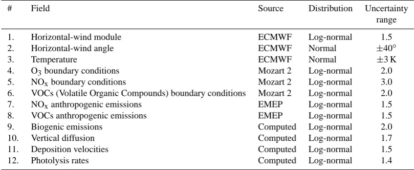
Table 2. Perturbation of input data. The last column is the parameterαthat defines the uncertainty range. If the median value of a normally-distributed random variablepˆ isp, the probability thatpˆ∈ [p−2α,p+2α]is 0.95. Ifpˆ is log-normally distributed, the probability that

ˆ

p∈ [p/α,αp]is 0.95.

# Field Source Distribution Uncertainty

range

1. Horizontal-wind module ECMWF Log-normal 1.5

2. Horizontal-wind angle ECMWF Normal ±40◦

3. Temperature ECMWF Normal ±3 K

4. O3boundary conditions Mozart 2 Log-normal 2.0

5. NOxboundary conditions Mozart 2 Log-normal 3.0

6. VOCs (Volatile Organic Compounds) boundary conditions Mozart 2 Log-normal 2.0

7. NOxanthropogenic emissions EMEP Log-normal 1.5

8. VOCs anthropogenic emissions EMEP Log-normal 1.5

9. Biogenic emissions Computed Log-normal 2.0

10. Vertical diffusion Computed Log-normal 1.7

11. Deposition velocities Computed Log-normal 1.5

12. Photolysis rates Computed Log-normal 1.4

are fully correlated (correlation equals 1) for a normal distri-bution. In the log-normal case, lnp(t,x)ˆ and lnp(tˆ 0,x0)are fully correlated.

The list of the perturbed fields and the corresponding val-ues ofα are shown in Table 2. These values were used in the example (Sect. 4). The list of input fields includes me-teorological variables, the boundary conditions, the emis-sions for different species and variables related to chemi-cal species such as the deposition velocities or the photol-ysis rates. These input data come from different models (ECMWF, Mozart 2, EMEP) or are processed during the pre-processing.

Once the distribution and the parameterαare determined, the actual perturbation is not given by a random sampling ofγ. The actual perturbed value is randomly and uniformly selected in a set of three values: the unperturbed value (i.e., the median)p˜0=p, and two other pointsp˜1andp˜2defined below. The points are chosen so that the empirical mean and the empirical standard deviation are the same as the mean and the standard deviation ofpˆ, thus

– E(p)ˆ =p˜0+ ˜p1+ ˜p2

3 ;

– Var(p)ˆ =(p˜0− ¯p) 2₊₍_p_˜

1− ¯p)2+(p˜2− ¯p)2

2 .

In the case wherepˆ∼N(p,1₄α2): ˜

p0=p; ˜

p1=p−1₂α; ˜

p1=p+1₂α .

Whenpˆis log-normally distributed: ˜

p0=p; ˜ p1=p

√ αγ1_; ˜

p2=p √

αγ2_,

with

γ1=2log(3β−1−

√

1

2 )/logα; γ2=2log(3β−1+

√

1

2 )/logα , and

β =exp(1₈log2α); 1=4β4−7β2+6β−3.

3.1.1 Models automatic selection

The selection of the models to be included in the ensemble is carried out randomly. A probability is given to each option. The numbers between brackets in Table 1 are these probabil-ities. In any alternative, the sum of the probabilities equals 1. Each perturbation in the input data (Table 2) is uniformly selected from three possible values (Sect. 3.1). A model is defined once an option has been selected for any alternative (18 alternatives are shown in Table 1, 12 perturbations are listed in Table 2).

(7)

8 D. Garaud et V. Mallet: Ensemble generation

Database

Preprocessing

Vertical diffusion Emissions

Deposition velocities Photolysis rates . . .

Driver

Numerical solver

Postprocessing

Libraries

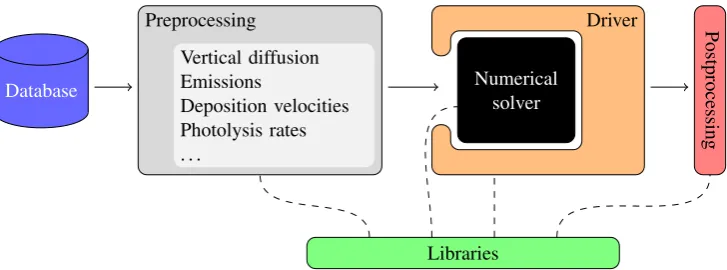
Fig. 1. A view on Polyphemus design: database storing all raw data, preprocessing stages for most physical computations, drivers in which the numerical solver is embedded, postprocessing and libraries that may be called at any time.

0

20

40

60

80

100 Number of simulations

70

75

80

85

90

95 Concentration

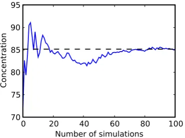
Fig. 2. The empirical mean of the ozone peaks averaged over all stations of network 1 and during 2001. It seems to have converged after about 70 simulations.

in section 4.3. We do not address more complex issues like

probabilistic forecasts, uncertainty estimation or sequential

aggregation.

495

4.1 Experiment Setup

In table 1, a probability is associated with every option. The

models are built according to these probabilities, but the

ac-tual frequency of an option in the 101-member ensemble may

differ slightly because of the random sampling. The

occur-500

rence frequency (in percentages) of each parameterization,

numerical option and field perturbation in the 101-member

ensemble are shown in table 3. For the field perturbations,

there are three options: no perturbation (raw data), increased

values in the field (

pα

if

p

≥

0 , or

p

+

α

) and decreased

505

values (section 3.1).

The six additional models can be seen as reference models.

They are built with the parameterizations that we trust the

most, and without any perturbation in the input field. If we

had to build a model for forecast, we would a priori choose

510

one of them. They are formed with the parameterizations

and numerical options from the first column of table 1 but

for the vertical diffusion parameterization and the mass

con-servation. Considering the three options for vertical

diffu-sion (line 5) and the two options for vertical-wind diagnosis

515

(line 13), six models may be constructed. These are listed in

table 4.

4.2 Evaluation of the Ensemble Members

4.2.1 Performance Measures

In order to evaluate a model performance,

n

available

obser-520

vations

oi

from different ground stations are compared with

the corresponding simulated concentrations

yi

, using

1. the root mean square error:

RMSE =

v

u

t

1 n

n

X

i=1

(

yi

−

oi

)

2

;

2. the correlation:

corr =

P

n

i=1

(

yi

−

y

¯

) (

oi

−

o

¯

)

q

P

n

i=1

(

yi

−

y

¯

)

2

q

P

n

i=1

(

oi

−

o

¯

)

2

,

where

o

¯

=

P

n

i=1

oi

and

y

¯

=

P

n

i=1

yi

;

3. the bias factor:

BF =

1 n

n

X

i=1

yi

oi

.

In practice, not all observations are retained. Stations that

fail to provide observations at over 10% of all considered

525

dates are discarded as these stations may not be reliable.

For ozone, the observations from three networks are

con-sidered:

Fig. 1. A view on Polyphemus design: database storing all raw data, preprocessing stages for most physical computations, drivers in which

the numerical solver is embedded, postprocessing and libraries that may be called at any time.

step tends to 0. Therefore, a higher probability is associ-ated with the time step fixed to 600 s. Another example is the chemical mechanism RACM which is more detailed than RADM 2, and which has shown slightly better results in sev-eral studies (Gross and Stockwell, 2003).

3.2 Technical aspects

The structure of the Polyphemus system contains four (mostly) independent levels: data management, physical pa-rameterizations, numerical solvers and high-level methods such as data assimilation. Figure 1 illustrates the structure of the modeling platform.

During the first stage, several C++ programs carry out the preprocessing. This is the most important part of the sim-ulation process, both in terms of simsim-ulation definition (the physics is set there) and computer code. Almost all terms of the reactive transport Eq. (1) are computed at this stage. The computations are split into several programs to ensure flexibility. For instance, there is one program to process land use cover (actually two programs: one for USGS data and another for GLCF data), one program for the main meteoro-logical fields, one program to compute biogenic emissions, another program for anthropogenic emissions, etc. Another example is the vertical diffusion coefficient: one program computes it with Louis parameterization and another with the Troen&Mahrt parameterization. In addition, these pro-grams have several options (e.g., the parameter p in the Troen&Mahrt parameterization, see Eq. 7). The use of multi-ple programs makes it an efficient system to build an ensem-ble. Adding new options is easy since one may simply add a new program (or add the option into an existing program). Moreover the computations are well managed. For example, if two models have the same options except the deposition velocity, all computations except those depending on depo-sition (i.e., the computation of the depodepo-sition velocities, and the numerical integration of the reactive transport equation) will be shared.

In the second stage, the numerical solver carries out the time integration of the reactive transport equation. The nu-merical solver is actually embedded in a structure called the “driver”. The driver is primarily in charge of perturbing the input data as detailed in Sect. 3.1.

At a postprocessing stage, the ensemble is completely gen-erated and the results are analyzed. At all stages, a few li-braries, mainly in C++ and Python, offer support, especially for data manipulation.

Disk space usage is optimized since the models can share part of their preprocessing. Moreover, the perturbed input fields (Table 2) are not stored; only the unperturbed fields (medians) are stored, and the driver applies the perturbations during the simulation.

Python scripts generate the identities (i.e., the set of op-tions and perturbaop-tions) of all models to be launched. The corresponding configuration files are created. The scripts then launch the preprocessing programs and the simulations. The simulations can obviously be run in parallel, so the scripts can launch the programs over SSH on different ma-chines and processors. The only constraint lies in the de-pendencies between the programs: e.g., the deposition ve-locities must be computed after the meteorological fields be-cause they depend on winds (among other fields). Groups of programs are defined with different priorities, and the scripts launch one group after the other. It is possible to relaunch parts of the ensemble computations. It is also possible to add new models (new simulations) after an initial ensemble has been generated. The Python code is available in the module EnsembleGeneration, from Polyphemus 1.5.

The same approach may be applied to another modeling system providing enough options (in the model formulation) are available. This requires that significant diversity is main-tained in the system. In particular, when a new formulation (e.g., a more accurate chemistry) is developed, the previous formulation should remain available to the user. The ratio-nale is that, while a formulation may seem better from a

(8)

Number of simulations

Concentration

Fig. 2. The empirical mean of the ozone peaks averaged over all

stations of network 1 and during 2001. It seems to have converged after about 70 simulations.

deterministic point of view (based on a priori considerations or on performance analysis), the previous formulation still has a significant probability (though lower than that of the new formulation) from a stochastic point of view.

4 An example of 101-member ensemble

With the previous method, about 620 billion models can be generated. An ensemble of 101 models is built and run throughout the year 2001 over Europe ([10.75◦W, 22.75◦E]×[34.75◦N, 57.75◦N]). The models are not sim-plified to reduce the computational costs. All models have a 0.5◦ _{horizontal resolution, which is a usual resolution.}

Be-cause the total computational cost is high, the ensemble size is limited to 101 simulations. This size is enough at least for the spatio-temporal empirical mean (of ozone peaks) to converge, as shown in Fig. 2.

Six reference models are included in the ensemble. These models are not generated automatically, but each of them cor-responds to a possible combination of options in that they could have been selected by the automatic procedure.

Aerosols are not taken into account in these simulations. The output stored on disk are the hourly concentrations in the first layer for O3, NO, NO2 and SO2 – which already amounts to 45 Gb of data.

Section 4.1 briefly summarizes which members are in-cluded in the ensemble. Although this paper is a technical description of the ensemble generation procedure, we aim to provide insight into the ensemble structure. We review the performance of the models, compared to ground obser-vations, in Sect. 4.2. We analyze the spread of the ensemble in Sect. 4.3. We do not address more complex issues like probabilistic forecasts, uncertainty estimation or sequential aggregation.

4.1 Experiment setup

In Table 1, a probability is associated with every option. The models are built according to these probabilities, but the ac-tual frequency of an option in the 101-member ensemble may differ slightly because of the random sampling. The occur-rence frequency (in percentages) of each parameterization, numerical option and field perturbation in the 101-member ensemble are shown in Table 3. For the field perturbations, there are three options: no perturbation (raw data), increased values in the field (pαifp≥0, orp+α) and decreased val-ues (Sect. 3.1).

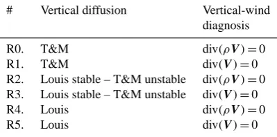
The six additional models can be seen as reference models. They are built with the parameterizations that we trust the most, and without any perturbation in the input field. If we had to build a model for forecast, we would a priori choose one of them. They are formed with the parameterizations and numerical options from the first column of Table 1 but for the vertical diffusion parameterization and the mass con-servation. Considering the three options for vertical diffu-sion (line 5) and the two options for vertical-wind diagnosis (line 13), six models may be constructed. These are listed in Table 4.

4.2 Evaluation of the ensemble members

4.2.1 Performance measures

In order to evaluate a model performance,navailable obser-vationsoi from different ground stations are compared with the corresponding simulated concentrationsyi, using

1. the root mean square error:

RMSE=

v u u t

1 n

n

X

i=1

(yi−oi)2;

2. the correlation: corr=

Pn

i=1(yi− ¯y)(oi− ¯o)

q Pn

i=1(yi− ¯y)2

q Pn

i=1(oi− ¯o)2

,

whereo¯=Pn

i=1oiandy¯=Pn_i=1yi; 3. the bias factor:

BF=1 n

n

X

i=1 yi

oi

.

(9)

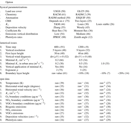
Table 3. Occurrence frequency of each parameterization, numerical option and field perturbation for the 101-member ensemble. As for the

perturbations, “raw” means no perturbation, “raw−” means lower value after perturbation (p/αorp−α) and “raw+” means higher value after perturbation (pαorp+α).

# Option

1. Land use cover USGS (50) GLCF (50)

2. Chemistry RACM (61) RADM 2 (39)

3. Attenuation RADM method (50) ESQUIF (50)

4. CRH Depends onσ(75) Two layers (25)

5. Kz T&M (44) Louis (30) Louis stable (26)

6. Deposition velocity Zhang (55) Wesely (45) 7. Coefficient Ra Heat flux (74) Moment flux (36) 8. Emissions vertical distribution Low (54) Medium (46) 9. Photolysis rates JPROC (88) Zenith angle (12) Numerical issues

10. Time step 600 s (91) 1200 s (9)

11. Vertical resolution 5 layers (48) 9 layers (52)

12. First layer height 50 m (40) 40 m (60)

13. Vertical-wind diagnosis div(ρV )=0 (52) div(V )=0 (48) 14. MinimalKz(m2s−1) 0.2 (66) 0.5 (34)

15. MinimalKzin urban area (m2s−1) 0.2 (30) 0.5 (35) 1.0 (35) 16. Vertical application of minimalKz Yes (84) No (16)

17. Exponentp 2 (75) 3 (25)

18. Boundary layer height raw value (61) +10% (18) –10% (7) +20% (14) Input data

19. Temperature (K) raw (39) raw−(34) raw+(27)

20. Horizontal-wind angle (degrees) raw (35) raw−(31) raw+(34) 21. Horizontal-wind velocity (m s−1) raw (36) raw−(40) raw+(24)

22. Kz(m2s−1) raw (33) raw−(32) raw+(35)

23. O3boundary conditions (µg m−3) raw (33) raw−(36) raw+(31) 24. NOxboundary conditions (µg m−3) raw (29) raw−(35) raw+(36) 25. VOCs boundary conditions (µg m−3) raw (35) raw−(37) raw+(28)

26. Biogenic emissions raw (34) raw−(28) raw+(38)

27. NOxemissions raw (34) raw−(35) raw+(31)

28. VOCs emissions raw (27) raw−(25) raw+(48)

29. Deposition velocities (cm s−1) raw (35) raw−(32) raw+(33)

30. Photolysis rates raw (34) raw−(37) raw+(29)

For ozone, the observations from three networks are con-sidered:

– Network 1 is composed of 243 urban and regional tions, primarily in France and Germany (116 and 81 sta-tions respectively). It provides about 1 365 000 hourly concentrations and 61 000 peaks.

– Network 2 includes 96 EMEP stations (regional stations distributed over Europe), with about 776 700 hourly ob-servations and 33 300 peaks.

– Network 3 includes 371 urban and regional stations in France. It provides 2 800 000 hourly measurements and 122 000 peaks. Note that it includes most of the French stations of network 1.

4.2.2 The models’ performance on ozone

Table 5 shows the performance of the six reference mod-els for ozone and of the best model in the ensemble. The best model is selected with respect to the RMSE for the

(10)

Table 4. Description of the 6 reference models.

# Vertical diffusion Vertical-wind diagnosis

R0. T&M div(ρV)=0

R1. T&M div(V)=0

R2. Louis stable – T&M unstable div(ρV)=0 R3. Louis stable – T&M unstable div(V)=0

R4. Louis div(ρV)=0

R5. Louis div(V)=0

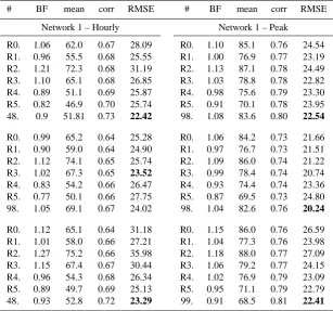
considered network and target (ozone peaks or ozone hourly concentrations). It is noteworthy that, except for network 2 and for hourly concentrations, there is always at least one model in the 101-member ensemble which is better than the six reference models (according to the RMSE and the cor-relation). The automatic generation of 101 models therefore created models that are as good as or better than the models derived from experience.

It also generated models with poor performance. Figure 3 shows the performance of the 101 models sorted according to the mean, biais factor, correlation and RMSE. The perfor-mance can obviously vary greatly.

4.2.3 The best model

In this section, we define the “best model” as the model with the lowest RMSE. Of course, it depends on the target (the network, the pollutant, the time period), and consider-ing the RMSE only is not enough to identify the best model, if any can be identified, as a modeler would do. Still this gives insights on the performance of models automatically generated.

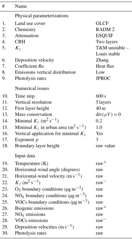
Model 98 in the 101-member ensemble is the best model for ozone peaks on network 1, for ozone hourly concentra-tions and ozone peaks on network 2 (Table 5). For these tar-gets, it beats the reference models. Several parameterizations and numerical options of model 98 are the same as those of the reference models (photolysis rates, deposition velocities, time step, etc.), but several selected options are unexpected. For instance, its chemical mechanism is RADM 2, and four fields are perturbed. See Table 6 for the complete description of model 98. It is interesting to note that (1) the random sam-pling generates several models with good performance (com-pared to the observations, with the RMSE), (2) the random sampling generates a model with lower square errors (over a long time period) than the models tuned by the modelers.

Among the 101 simulations, the median RMSE is about 27 µg m−3and the median correlation is close to 0.73.

10 D. Garaud et V. Mallet: Ensemble generation

centrations). It is noteworthy that, except for network 2 and 545

for hourly concentrations, there is always at least one model in the 101-member ensemble which is better than the six ref-erence models (according to the RMSE and the correlation). The automatic generation of 101 models therefore created models that are as good as or better than the models derived 550

from experience.

It also generated models with poor performance. Figure 3 shows the performance of the 101 models sorted according to the mean, biais factor, correlation and RMSE. The perfor-mance can obviously vary greatly.

555

4.2.3 The Best Model

In this section, we define the “best model” as the model with the lowest RMSE. Of course, it depends on the target (the network, the pollutant, the time period), and considering the RMSE only is not enough to identify the best model, if any 560

can be identified, as a modeler would do. Still this gives insights on the performance of models automatically gener-ated.

Model 98 in the 101-member ensemble is the best model for ozone peaks on network 1, for ozone hourly concentra-565

tions and ozone peaks on network 2 (table 5). For these tar-gets, it beats the reference models. Several parameterizations and numerical options of model 98 are the same as those of the reference models (photolysis rates, deposition velocities, time step, . . . ), but several selected options are unexpected. 570

For instance, its chemical mechanism is RADM 2, and four fields are perturbed. See table 6 for the complete description of model 98. It is interesting to note that (1) the random sam-pling generates several models with good performance (com-pared to the observations, with the RMSE), (2) the random 575

sampling generates a model with lower square errors (over a long time period) than the models tuned by the modelers.

Among the 101 simulations, the median RMSE is about

27µg m−3_{and the median correlation is close to}₀_.₇₃_.

4.3 Ensemble Variability 580

Every model in the ensemble is unique, but one may ask whether the ensemble contains enough information and has a rich structure. For example, the ensemble should not be clus-tered into distinct groups of similar models. One measure of the difference between two models is the number of options 585

that differ between them. Interestingly enough, two models with a similar RMSE can be made with many different op-tions: for example models 98 and 58, which have close RM-SEs (22.54and23.65respectively, ozone peak, network 1), are generated with 17 different options (out of 30) shown in 590

table 7. This fact can be observed with the whole ensemble. In figure 4, the models are sorted according to their RMSE for ozone peaks on network 1 (model 0 has the lowest RMSE, and model 100 has the highest RMSE), and the matrix of the differences between the models (measured with the number 595

0

20

40

60

80

100 Sorted Member

50

60

70

80

90

100

110

120

130 Mean

observation

simulation

0

20

40

60

80

100 Sorted Member

0.6

0.8

1.0

1.2

1.4

1.6

1.8 Biais Factor

0

20

40

60

80

100 Sorted Member

0.4

0.5

0.6

0.7

0.8 Corrleation

0

20

40

60

80

100 Sorted Member

20

25

30

35

40

45

50

55

60 RMSE

Fig. 3. Mean (µg m−3), biais factor, correlation and RMSE (µg m−3) for ozone peaks on network 1. In each plot, the mod-els are sorted according to the indicator.

(11)

Table 5. Statistical measures for the 6 reference models and the best model from the 101-member ensemble, for hourly ozone concentrations

and hourly ozone peaks. R0–5 refer to the 6 reference models.

# BF mean corr RMSE # BF mean corr RMSE

Network 1 – Hourly Network 1 – Peak R0. 1.06 62.0 0.67 28.09 R0. 1.10 85.1 0.76 24.54 R1. 0.96 55.5 0.68 25.55 R1. 1.00 76.9 0.77 23.19 R2. 1.21 72.3 0.68 31.19 R2. 1.13 87.1 0.78 24.49 R3. 1.10 65.1 0.68 26.85 R3. 1.03 78.8 0.78 22.82 R4. 0.89 51.1 0.69 25.87 R4. 0.98 75.6 0.79 23.30 R5. 0.82 46.9 0.70 25.74 R5. 0.91 70.1 0.78 23.95 48. 0.9 51.81 0.73 22.42 98. 1.08 83.6 0.80 22.54

R0. 0.99 65.2 0.64 25.28 R0. 1.06 84.2 0.73 21.66 R1. 0.90 59.0 0.64 24.90 R1. 0.97 76.7 0.73 21.51 R2. 1.12 74.1 0.65 25.74 R2. 1.09 86.0 0.74 21.22 R3. 1.02 67.3 0.65 23.52 R3. 0.99 78.4 0.74 20.74 R4. 0.83 54.2 0.66 26.47 R4. 0.93 74.4 0.74 23.36 R5. 0.77 50.1 0.66 27.75 R5. 0.87 69.5 0.73 24.80 98. 1.05 69.1 0.67 24.02 98. 1.04 82.6 0.76 20.24

R0. 1.12 65.1 0.64 31.18 R0. 1.15 86.0 0.76 26.59 R1. 1.01 58.0 0.66 27.21 R1. 1.04 77.3 0.76 23.98 R2. 1.27 75.2 0.66 35.98 R2. 1.18 88.0 0.77 27.09 R3. 1.15 67.4 0.67 30.44 R3. 1.06 79.2 0.77 24.15 R4. 0.96 54.3 0.68 26.34 R4. 1.02 76.9 0.79 23.09 R5. 0.89 49.7 0.69 25.13 R5. 0.95 71.1 0.79 22.79 48. 0.93 52.8 0.72 23.29 99. 0.91 68.5 0.81 22.41

4.3 Ensemble variability

Every model in the ensemble is unique, but one may ask whether the ensemble contains enough information and has a rich structure. For example, the ensemble should not be clustered into distinct groups of similar models. One mea-sure of the difference between two models is the number of options that differ between them. Interestingly enough, two models with a similar RMSE can be made with many dif-ferent options: for example models 98 and 58, which have close RMSEs (22.54 and 23.65 respectively, ozone peak, net-work 1), are generated with 17 different options (out of 30) shown in Table 7. This fact can be observed with the whole ensemble. In Fig. 4, the models are sorted according to their RMSE for ozone peaks on network 1 (model 0 has the low-est RMSE, and model 100 has the highlow-est RMSE), and the matrix of the differences between the models (measured with the number of differing options) is shown. No overall struc-ture can be identified. This tends to show that quite different models can achieve similar performance. The RMSE, seen as a function of the parameters, seems to have many local minima.

Fig. 4. Matrix of the number of different options between two

mod-els. The models are sorted according to the RMSE (from the best to the worst value).

On the other hand, the output of the best models are corre-lated. This is shown in Fig. 5 with the correlation computed with all ozone peaks observed in network 1. Two skillful models therefore have a similar spatio-temporal variability.

(12)

Fig. 5. Matrix of correlation between all observed ozone peaks (on

network 1) and the corresponding model-concentrations. The mod-els are sorted according to the RMSE (from the best to the worst value).

Table 6. Description of the best model.

# Name

1. Land use cover GLCF

2. Chemistry RADM 2

3. Attenuation ESQUIF

4. CRH Two layers

5. Kz T&M unstable –

Louis stable

6. Deposition velocity Zhang

7. Coefficient Ra Heat flux

8. Emissions vertical distribution Low

9. Photolysis rates JPROC

Numerical issues

10. Time step 600 s

11. Vertical resolution 5 layers

12. First layer height 40 m

13. Mass conservation div(ρV )=0 14. MinimalKz(m2s−1) 0.2 15. MinimalKzin urban area (m2s−1) 1.0 16. Vertical application for minimalK_z Yes

17. Exponentp 3

18. Boundary layer height raw value

Input data

19. Temperature (K) raw+

20. Horizontal-wind angle (degrees) raw 21. Horizontal-wind velocity (m s−1) raw

22. K_z(m2s−1) raw−

23. O3boundary conditions (µg m−3) raw

24. NOxboundary conditions (µg m−3) raw

25. VOCs boundary conditions (µg m−3) raw

26. Biogenic emissions raw+

27. NOxemissions raw

28. VOCs emissions raw−

29. Deposition velocities (m s−1) raw

30. Photolysis rates raw

Table 7. A comparison between the model 98 and 58.

Name Model 98 Model 58

Chemical Mechanism RADM 2 RACM

Cloud attenuation ESQUIF RADM

Critical relative humidity on 2 layers withσ

Vertical diffusion Troen & Mahrt Louis unstable –

Louis stable

Coefficient Ra Heat flux Moment flux Vertical resolution 5 levels 9 levels

Time step 600 s 1200 s

ExponentpforKz 3 2

First layer height 40 m 50 m

MinimalKzin urban area 1.0 0.5

Temperature raw+ raw

NO_xboundary conditions raw raw+ VOCs boundary conditions raw raw+

Biogenic emissions raw+ raw

NO_xemissions raw raw+

VOCs emissions raw− raw

Deposition velocities raw raw+

These high correlations are partly due to the structure of ozone fields. Because of the physical constraints, two reason-able ozone fields necessarily share a set of common features, such as higher concentrations in the south compared to the north, or low concentrations at high NO emission sources. However, two skillful models can show significant differ-ences in their spatial patterns, as Fig. 6 demonstrates.

Figures 7, 8, 9, and 10 show the temporal mean of the con-centration map of the fifth reference model and of a model from the 101-member ensemble, for O3, NO, NO2and SO2 respectively. Again, the physical constraints make the mod-els reproduce specific features, like high NO concentrations only at emission locations, but significant differences are found.

Figures 11 shows the mean daily profiles of all models from the 101-member ensemble, for O3, NO, NO2and SO2 respectively. For the species O3and NO2, the daily profiles are computed on network 3 whereas the daily profiles for the species NO and SO2 are computed with all cells. All models produce a similar profile shape, which is due to the physical phenomena accounted for in every model and the fact that these profiles are highly averaged (whole year, and full domain or all stations). The means can differ a lot, and, obviously, not all models are equally likely.

(13)

D. Garaud and V. Mallet: Ensemble generation14 D. Garaud et V. Mallet: Ensemble generation 81

−10 −5 0 5 10 15 20 35 40 45 50 55 20 40 60 80 100 120 140 160 180

Fig. 6.Ozone map of model 98 (left) and model 58 (right), on 5 May 2001 at 17:00 UT. Both models show good performance, but they can

produce ozone fields that differ significantly.

− 10 −5

0 5 10 15 20 35 40 45 50 55 15.0 28.5 42.0 55.5 69.0 82.5 96.0 − 10 −5

0 5 10 15 20 35 40 45 50 55 15.0 28.5 42.0 55.5 69.0 82.5 96.0

Fig. 7.Temporal average of ozone map for reference model 5 (left) and for model 76 of the 101-member ensemble (right).

−

10 −

5 0 5 10 15 20

35 40 45 50 55 0 9 18 27 36 45 54 − 10 −

5 0 5 10 15 20

35 40 45 50 55 0 9 18 27 36 45 54

Fig. 8.Temporal average ofNOmap for reference model 5 (left) and for model 52 of the 101-member ensemble (right).

Fig. 6. Ozone map of model 98 (left) and model 58 (right), on 5 May 2001 at 17:00 UT. Both models show good performance, but they can

−

10 −

5 0 5 10 15 20

35 40 45 50 55 20 40 60 80 100 120 140 160 180 − 10 −

5 0 5 10 15 20

35 40 45 50 55 20 40 60 80 100 120 140 160 180

Fig. 6.Ozone map of model 98 (left) and model 58 (right), on 5 May 2001 at 17:00 UT. Both models show good performance, but they can

−10

−

5 0 5 10 15 20 35 40 45 50 55 15.0 28.5 42.0 55.5 69.0 82.5 96.0 −10 −

5 0 5 10 15 20 35 40 45 50 55 15.0 28.5 42.0 55.5 69.0 82.5 96.0

−10 −5 0 5 10 15 20 35 40 45 50 55 0 9 18 27 36 45 54 − 10 −

5 0 5 10 15 20

35 40 45 50 55 0 9 18 27 36 45 54

Fig. 7. Temporal average of ozone map for reference model 5 (left) and for model 76 of the 101-member ensemble (right).

−10 −5 0 5 10 15 20

35 40 45 50 55 20 40 60 80 100 120 140 160 180

−10 −5 0 5 10 15 20

35 40 45 50 55 20 40 60 80 100 120 140 160 180

Fig. 6.Ozone map of model 98 (left) and model 58 (right), on 5 May 2001 at 17:00 UT. Both models show good performance, but they can produce ozone fields that differ significantly.

−10 −5 0 5 10 15 20 35 40 45 50 55 15.0 28.5 42.0 55.5 69.0 82.5 96.0

−10 −5 0 5 10 15 20

35 40 45 50 55 0 9 18 27 36 45 54 −10 −

5 0 5 10 15 20 35 40 45 50 55 0 9 18 27 36 45 54

Fig. 8. Temporal average of NO map for reference model 5 (left) and for model 52 of the 101-member ensemble (right)._{D. Garaud et V. Mallet: Ensemble generation} ₁₅

−

10 −

5 0 5 10 15 20 35 40 45 50 55 0 12 24 36 48 60 72 − 10 −

5 0 5 10 15 20 35 40 45 50 55 0 12 24 36 48 60 72

Fig. 9.Temporal average ofNO2map for reference model 5 (left) and for model 90 of the 101-member ensemble (right).

−10

−

5 0 5 10 15 20 35 40 45 50 55 0.0 19.5 39.0 58.5 78.0 97.5 117.0 −10 −

5 0 5 10 15 20 35 40 45 50 55 0.0 19.5 39.0 58.5 78.0 97.5 117.0

Fig. 10.Temporal average ofSO2map for reference model 5 (left) and for model 88 of the 101-member ensemble (right).

Appendix A

700

Emissions from EMEP

As described in section 2, anthropogenic emissions are pro-vided by EMEP. The vertical distribution of the pollutants depends on SNAP category. Two vertical distributions are

705

used in this paper: a “low distribution” and a “medium

distribution”—see table A1.

Acknowledgements. We thank Richard James for proofreading the paper.

References

710

Beekmann, M. and Derognat, C.: Monte Carlo uncertainty anal-ysis of a regional-scale transport chemistry model constrained by measurements from the atmospheric pollution over the Paris area (ESQUIF) campaign, Journal of Geophysical Research, 108, 8,559, doi:10.1029/2003JD003391, 2003.

715

Boutahar, J., Lacour, S., Mallet, V., Qu´elo, D., Roustan, Y., and Sportisse, B.: Development and validation of a fully modular platform for numerical modelling of air pollution: POLAIR, In-ternational Journal of Environment and Pollution, 22, 17–28, 2004.

720

Byun, D. W. and Ching, J. K. S., eds.: Science algorithms of the EPA models-3 community multiscale air quality (CMAQ) mod-eling system, U.S. Environmental Protection Agency, Washing-ton, 1999.

Chang, J., Brost, R., Isaken, I., Madronich, S., Middleton, P., Stock-725

well, W., and Walcek, C.: A three-dimensional Eulerian acid de-position model: physical concepts and formulation, Journal of Fig. 9. Temporal average of NO2map for reference model 5 (left) and for model 90 of the 101-member ensemble (right).

(14)

82 D. Garaud and V. Mallet: Ensemble generation −

10 −5

0 5 10 15 20 35 40 45 50 55 0 12 24 36 48 60 72 − 10 −

5 0 5 10 15 20 35 40 45 50 55 0 12 24 36 48 60 72

Fig. 9.Temporal average ofNO2map for reference model 5 (left) and for model 90 of the 101-member ensemble (right).

−10 −5 0 5 10 15 20 35 40 45 50 55 0.0 19.5 39.0 58.5 78.0 97.5 117.0

Fig. 10.Temporal average ofSO2map for reference model 5 (left) and for model 88 of the 101-member ensemble (right).

Appendix A

700

Emissions from EMEP

As described in section 2, anthropogenic emissions are pro-vided by EMEP. The vertical distribution of the pollutants depends on SNAP category. Two vertical distributions are

705

used in this paper: a “low distribution” and a “medium

distribution”—see table A1.

Acknowledgements. We thank Richard James for proofreading the paper.

References

710

Beekmann, M. and Derognat, C.: Monte Carlo uncertainty anal-ysis of a regional-scale transport chemistry model constrained by measurements from the atmospheric pollution over the Paris area (ESQUIF) campaign, Journal of Geophysical Research, 108, 8,559, doi:10.1029/2003JD003391, 2003.

715

Boutahar, J., Lacour, S., Mallet, V., Qu´elo, D., Roustan, Y., and Sportisse, B.: Development and validation of a fully modular platform for numerical modelling of air pollution: POLAIR, In-ternational Journal of Environment and Pollution, 22, 17–28, 2004.

720

Byun, D. W. and Ching, J. K. S., eds.: Science algorithms of the EPA models-3 community multiscale air quality (CMAQ) mod-eling system, U.S. Environmental Protection Agency, Washing-ton, 1999.

Chang, J., Brost, R., Isaken, I., Madronich, S., Middleton, P.,

Stock-725

well, W., and Walcek, C.: A three-dimensional Eulerian acid de-position model: physical concepts and formulation, Journal of

Fig. 10. Temporal average of SOD. Garaud et V. Mallet: Ensemble generation2map for reference model 5 (left) and for model 88 of the 101-member ensemble (right). 17

0 5 10 15 20

Hour 20 40 60 80 100 120 Concentration

0 5 10 15 20

Hour 0.0 0.5 1.0 1.5 2.0 2.5 3.0 3.5 4.0 4.5 Concentration

0 5 10 15 20

Hour 0 5 10 15 20 25 30 35 40 45 Concentration

0 5 10 15 20

Hour 0 5 10 15 20 25 30 Concentration

Fig. 11.Daily profile for ozone (network 3),NO,NO2(network 3)

andSO2. The profile is computed at observation stations forO3

−

10 −

5 0 5 10 15 20 35

40 45 50 55

10 20 30 40 50 60 70 80 90 100

−

10 −

5 0 5 10 15 20 35

40 45 50 55

0 10 20 30 40 50 60 70 80 90

−

10 −

5 0 5 10 15 20 35

40 45 50 55

0 10 20 30 40 50 60 70 80 90 100

Fig. 12. Maps of best-model indexes. In each grid cell of the domain, the color shows which model (marked with its index, in

J0,100K) gives the best ozone peak forecast on 1 June, 11 June and

13 June 2001 at the closest station to the cell center. It shows that many models can deliver the best forecast at some point. Stations of network 1 are used. Of course, the colors are only reliable in

D. Garaud et V. Mallet: Ensemble generation 17

0 5 10 15 20

andNO2. It is computed with all computed values (that is, from all

grid cells) forNOandSO2.

−10 −5 0 5 10 15 20 35

40 45 50 55

10 20 30 40 50 60 70 80 90 100

−

10 −5

0 5 10 15 20 35

40 45 50 55

0 10 20 30 40 50 60 70 80 90

−

10 −

5 0 5 10 15 20 35

40 45 50 55

0 10 20 30 40 50 60 70 80 90 100

13 June 2001 at the closest station to the cell center. It shows that many models can deliver the best forecast at some point. Stations of network 1 are used. Of course, the colors are only reliable in regions that contain stations.

0 5 10 15 20

− 10 −5

0 5 10 15 20 35

40 45 50 55

10 20 30 40 50 60 70 80 90 100

−

10 −

5 0 5 10 15 20 35

40 45 50 55

0 10 20 30 40 50 60 70 80 90

−

10 −

5 0 5 10 15 20 35

40 45 50 55

0 10 20 30 40 50 60 70 80 90 100

0 5 10 15 20

−

10 −

5 0 5 10 15 20 35

40 45 50 55

10 20 30 40 50 60 70 80 90 100

−10 −5 0 5 10 15 20 35

40 45 50 55

0 10 20 30 40 50 60 70 80 90

−

10 −

5 0 5 10 15 20 35

40 45 50 55

0 10 20 30 40 50 60 70 80 90 100

Fig. 11. Daily profile for ozone (network 3), NO, NO2(network 3) and SO2. The profile is computed at observation stations for O3and NO2. It is computed with all computed values (that is, from all grid cells) for NO and SO2.

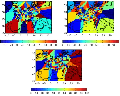
still likely to produce the best forecast. This can be verified with a “map of the best-model index”. At a given date, the best model in each grid cell is determined as follows. The concentrations of the models and the observed concentration at the closest station (to the grid cell) are compared. The model that produces the closest concentration to the observed concentration is considered as the best model in the grid cell. Hence, in every grid cell, one “best model” is determined. A color is associated to each model (actually each model index) to generate the maps in Fig. 12. These maps show the best model for three different dates in June 2001. The best model varies frequently from one grid cell to another, and from one date to another. This shows that many models bring useful information, at least in some regions or on given dates.

5 Conclusions

This paper describes how a large ensemble may be automat-ically generated using the Polyphemus system. Contrary to most traditional approaches, which are based on perturba-tions of input data only, or on small ensembles of models from different teams, our approach takes into account all sources of uncertainties at once: input data, physical formu-lation and numerical formuformu-lation. Each member of the en-semble is a complete chemistry-transport model whose con-tents are clearly defined within the modeling platform. In this context, the ensemble and the differences between its members can be rigorously analyzed, and also controlled through the probabilities associated with every option. Our approach tries to combine the flexibility of Monte Carlo