http://dx.doi.org/10.9717/JMIS.2017.4.4.219
219
I. INTRODUCTION
In the pattern recognition system, it is considered that is the characteristic of the vectors on the image. The number of the characteristic vectors that is composed to the dimension of vectors is also very important in the rate of recognition. As the more characteristic factors is, it will be affected weakness on the system. Furthermore, it will be slow to read the learning.
g and recognition rate of the image and we need to the group of the learning for the modeling. The number of the characteristic vectors is getting more i.e. the characteristic vectors that is composed the dimensions of the vectors is higher. On the most of pattern recognition, the capacity of the pattern recognition is better until some range, but it will happen rather decreasing than increasing. By the principle components analysis, what is the optimal reduction from higher dimension of characteristic vectors to lower dimension of characteristic vectors. The Principle component is one of multivariate data processing methods that reduced from high dimension to low dimension. Characteristic Data is presented standard axis as many as
the number of dimensions of the characteristic vectors. The n-dimension is presented by the data of n standard axes. If the dimension is reduced, it will be reduced the number of the standard axes. Therefore, the standard axes of statistics multivariate data is to project on a characteristic vector, it will be reduced. PCA (Principle Component Algorithm) is to rearrange the characteristic vectors and transform a standard axis based on the set of uncorrelated variates. In this paper, we analyze the extractions of the characteristic vectors and the algorithm in the parallel cases.
II. DEVELOPMENT OF IMAGE
RECONGNITION’S PARALLEL
ALOGORITHM
Why do we need this method to rearrange the characteristic vectors? We need the simple example the concrete the cases. We have a simple example of PCA as below:
An Application of a Parallel Algorithm on an Image Recognition
Ran Baik
1Abstract
This paper is to introduce an application of face recognition algorithm in parallel. We have experiments of 25 images with different motions and simulated the image recognitions; grouping of the image vectors, image normalization, calculating average image vectors, etc. We also discuss an analysis of the related eigen-image vectors and a parallel algorithm. To develop the parallel algorithm, we propose a new type of initial matrices for eigenvalue problem. If A is a symmetric matrix, initial matrices for eigen value problem are investigated: the "optimal" one, which minimize CAF and the "super optimal”, which minimize
F A C
I 1 . In this paper, we present a general new approach
to the design of an initial matrices to solving eigenvalue problem based on the new optimal investigating C with preserving the characteristic of the given matrix A. Fast all resulting can be inverted via fast transform algorithms with O(N log N) operations.
Key Words: pattern recognition, eigenvalue problem, principle components, initial matrices, Symmetric matrices, Gram-Schmidt.
Manuscript received December 28, 2017; Revised December 29, 2017; Accepted December 30, 2017. (ID No. JMIS-2017-0058)
Corresponding Author: Ran Baik, #417 Eodeung-daero, Gwangsan-gu, Gwangju, Republic of Korea, Tel: 82-62-940-5425, E-mail:[email protected].
220
2.1. Distributions and transformations of group of the characteristic vectors
A group of random vectors that the value is below will be distributed by given condition.
(1) To produce natural vector sets
(2) To rearrange the given vectors from (1) that average of all vectors are zero.
(3) To reproduce the vectors that the radius from origin is less than 0.5 and ignore others, i.e. greater than 0.5. We can scatter the data that is composed 2-dimension of 1000 random vectors (Figure 1)
Fig 1. Distribution of set of vectors
Also we consider the step to figure out from x-y coordinates to polar coordinates transformations of the distribution of the given set of the vectors (Fig. 2 and Fig. 3).
In this work, we need to compute the eigenvalues of a covariance matrix to know the principal components of the images. Furthermore, we use the eigenvectors from the eigenvalues to get the information of Principle components.
Fig 2. Steps for transformation of the set of vectors.
Fig 3. Principle components of the given vectors.
There are several methods to solve the eigen problem, but there are sequential processes to get all eigenvalues. Also, the structure of the given matrix is broken to do for it. In our work, we want to keep the structure of the given matrix and develop the parallel algorithm. We compare the complexity to compute all eigenvalues of the given matrix between existing algorithm and our algorithm.
2.2. A Construction of an Image Recognition’s Algorithm
2.2.1 Development of an algorithm of eigenface on PCA
Each pixel of a face-image is composed of on the face space.
An eigenface is the base vectors which is composed the face space. The base vectors is presented the common characteristics among all candidate face images. The eigen face is produced from difference vectors between an average face image and each candidate face image. These are eigenvectors of the covariance matrix. Since a set of eigenvalues of the covariance matrix is a representation of the range of distribution of average face image, the eigenface which is composed the largest eigenvalue and its eigenvector is the closest face with the origin face. If the eigenvalue is getting smaller, it will decrease the characteristic of the face image. Therefore, we discuss the largest eigenvalue and the smallest eigenvalue of our face image and study the algorithm to compute them in this section.
We apply the algorithm for computing the largest eigenvalue and the smallest eigenvalue independently. We compare the difference between the largest eigenface and the smallest eigenface. We discuss analysis of the algorithm in parallel. First of all, we develop a method to compute the extreme eigenvalues. Ii is modified by Newton method with a parameter t. It is a procedure to develop the algorithm as follows;
We denote by the space of n-by-n symmetric matrices. We denote by σ(A) the set of eigenvalues of A∈ .
Let A∈ be a symmetric matrix. Then there is an orthogonality U = [U1,…., Un] ∈ such that
A
⋯ 0 ⋮ ⋱ ⋮ 0 ⋯
, ∈ .
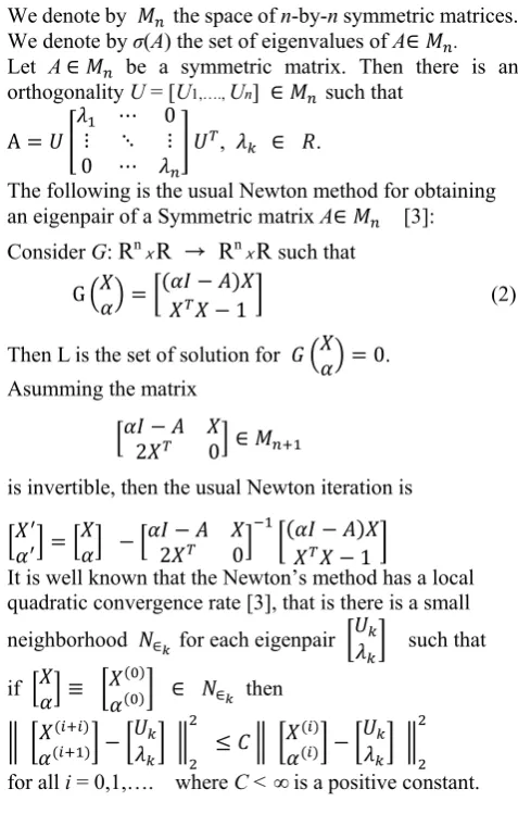
The following is the usual Newton method for obtaining an eigenpair of a Symmetric matrix A∈ [3]:
Consider G: RnⅹR → RnⅹR such that
G
1 (2)
Then L is the set of solution for 0. Asumming the matrix
2 0 ∈
is invertible, then the usual Newton iteration is
2 0 1
It is well known that the Newton’s method has a local quadratic convergence rate [3], that is there is a small neighborhood ∈ for each eigenpair such that
if ≡ ∈ ∈ then
for all i = 0,1,…. where C < ∞ is a positive constant.
http://dx.doi.org/10.9717/JMIS.2017.4.4.219
221
the eigenpair . Although the specific determination of each ∈ is an extremely difficult task, if the method
converges to a point in L then we know the rate of convergence will eventually be quadratic. It can be shown easily that the Newton’s method is not global.
We modify the Newton method in order to have a global convergence [2]. There are several considerations to give for the Modification.
First, under the modification we desire the pair gets closer to an eigenpair at each step of the iteration,
i.e., where is a
suitable distance measure from a point to L. It will ensure the points under the iteration remain in D. Second, we want to modify the method the least amount as possible in order to preserve the original properties of the Newton’s Method, for example, local quadratic convergence. Third, the modified method should be simple to implement, requires almost the same procedures as the original Newton iteration.
2.3 Newton Iteration and Its Modification
Consider the usual Newton iteration (2):
2 0 1
Choose a parameter t > 0 so that the method takes the form
2 0
0 0
0
1/ . (3)
Then ′
(4)
and 2 2 1 (5) Then the parameterized Newton method takes a form:
( , (6)
and . (7)
Now, suppose ∈ D and let L | ∈
, ‖ ‖ 1, and ∈ be the set of all eigenpairs of
A. Define a distance measure from a point to L by
≡ ‖ ‖ (8)
Clearly, 0, 0 implies ∈
, and : D → R is continuous (since D is compact, is actually uniformly continuous).
We have the following.
Lemma 1[4]: Let A∈ be Symmetric. Consider the parameterized Newton’s method
( , and , where
β , and
‖ ‖ / .
Then ′
′ is minimized at t = with
min ′
′ 1
/
.
Therefore, we have the following modification of the Newton’s method:
( (9)
. (10)
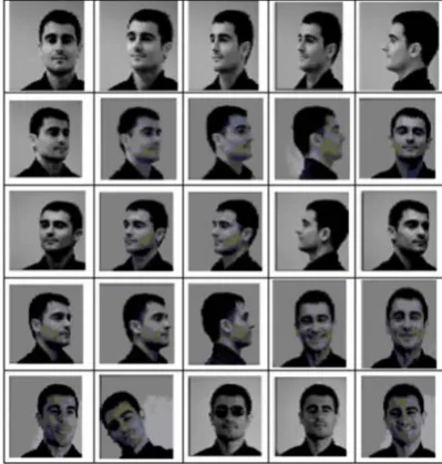
In this 2.3, we discuss it about an application of eigenfaces from 25 different expressions of a face.
2.4An application of the face recognition
There are 5 steps to construct for face images.
Step 1: An input of the origin images
The size of face image is NⅹN and the number of the face images that are recognized as candidates are M such that each is 1 column vector. Denote the set of face vectors that are recognized as candidates by S (Fig 4).
S , , , … , (11)
Fig 4. Recognition candidate face DB.
222 Step 2: Normalization of the image
We normalize the image on the basis of setting average and variance to reduce errors caused by the light and background (Figure 5).
Step 3: Computation of the average Face’s vector
We compute the average face vector from the face set S of recognition candidates (Figure 6).
Ψ ∑ (12)
Fig 6. Average face
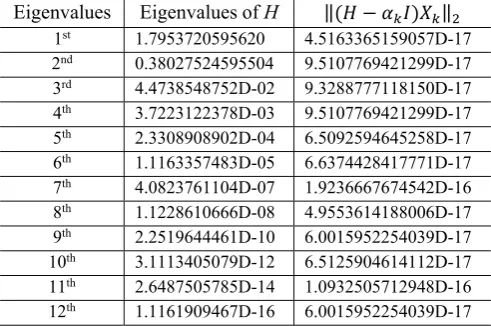
In the computation for eigenpairs we develop the parallel algorithm with modified Newton method each eigenpair. Even though, the given matrix is ill conditioned, we can get all eigenpairs. This is an ill-conditioned matrix case:
Example1: Let H
1 1/2 1/3 ⋯ 1/ 1/2 1/3 ⋱ ⋱ ⋮
⋮ ⋱ ⋱ ⋱ ⋮
⋮ ⋱ ⋱ ⋱ ⋮
1/ ⋯ ⋯ ⋯
be a
n by n Hilbert matrix H. The Hilbert matrix is a well-known example of an ill-conditioned positive. Because the smallest eigenvalue of H∈ is so near zero, many conventional algorithms produce = 0. Our method gives the following experimental results:
Set the convergence criterion, ε=2ⅹ10 , i.e.,
‖ ‖ .
Suppose D= | ∈ , , … , , ∈
, , , , … , , is the initial set of points where ei is
the ith column of the identity matrix and hi,i is the ith
diagonal entry of H.
Table 1: Eigenvalues of H12 by Modified Newton Method
Eigenvalues Eigenvalues of H ‖ ‖
1st 1.7953720595620 4.5163365159057D-17
2nd 0.38027524595504 9.5107769421299D-17
3rd 4.4738548752D-02 9.3288777118150D-17
4th 3.7223122378D-03 9.5107769421299D-17
5th 2.3308908902D-04 6.5092594645258D-17
6th 1.1163357483D-05 6.6374428417771D-17
7th 4.0823761104D-07 1.9236667674542D-16
8th 1.1228610666D-08 4.9553614188006D-17
9th 2.2519644461D-10 6.0015952254039D-17
10th 3.1113405079D-12 6.5125904614112D-17
11th 2.6487505785D-14 1.0932505712948D-16
12th 1.1161909467D-16 6.0015952254039D-17
If we have some clustering case on the target matrix, we can also overcome all eigenpairs[Figure 7].
Fig .7. MNM Process.
To overcome the lost eigenpairs from MNM by the Gram-Schmidt orthogonalization process.
Suppose both [x1, 1]T and [x2, 2] T converge to [U1,1]T. (i) Choose a vector x = x1 (or x2).
(ii) Apply the Gram-Schmidt orthogonalization process. z = x - < U1, x> U1, xx = z/ z 2
(iii) Apply MNM with [xx, 1 ]T (or [xx, 2]T ). [xx,1]T (or [xx, 2]T ) will converge to [U2, 2 ].
It is shown the MNM in (10), (11) and this is algorithm as below:
Modified Newton’s Algorithm Set α and x .
(α , x ) is an initial eigenpairs where α and
x , k = 1, …, n are the diagonal entries of the given matrix and , , … , .
For k = 1, …, n do (in parallel) For j = 1, … do until convergence (i) Solve for y , α
(ii) Compute β ∙
(iii) Compute β .
(iv) Compute
(v) Compute α α
End End
We apply the MNM(Modified Newton Method) to generate eigen-imgages at each step for image recognition problems.
In this case, we work to find the all eigenpairs of a covariance matrix which is generated by the characteristic vectors.
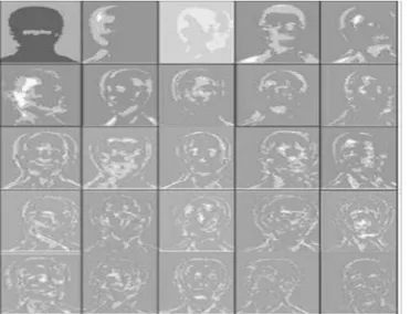
Step 4: Solving of the eigen problem of a Covariance Matrix C
We compute the eigenvalue and the corresponding eigenvectors of the covariance matrix C. It is based on our algorithm. The eigenvalue present an average face of the given image and it produce a eigen-face(Fig. 8).
http://dx.doi.org/10.9717/JMIS.2017.4.4.219
223
Fig. 8 Eigen-Faces
III. CONCLUSION
We can get each component to be projected by the eigenvalues after their new faces are input. It is shown how to compute each eigenface component as follows :
μ Ψ , k=1, 2, …, M′ (14)
M′ is the number that there are excluded the smallest eigenface corresponding the smallest eigenvalues. From the weight, we can get the component vector Ω of eigenface that are expressed input face images. If we get the set Ω , , … , , we can expect the errors as
follows Ω Ω .
Step 5: A Reconstruction of the given image
We compare the origin image and reconstructed image which is applied our algorithm (Figure 9).
Fig. 9. An Input image and reconstruction of a Face with the algorithm
REFERENCES
[1] A. Webb, Statistical Pattern Recognition, 2nd: John Wiley & Sons Inc., 2002.
[2] J. M. Ortega, Numerical Analysis, A Second Course: SIAM Series in Classical in Applied Mathematic:
Philadelphia, SIAM Publications, 1990.
[3] J. M. Ortega and W. C. Rheinboldt, Iterative Solution Of Nonlinear Equations In Several Variables: Academic Press, New York and London, 1970.
[4] R. Baik, K. Datta and Y. Hong, “Computing for Eigenpairs on Globally Convergent Iterative for Hermitian Matrices,” Lecture Note in Computer Science, vol. 3514, pp. 1- 8, 2005.
[5] Karabi Datta and Yoopyo Hong and Ran Baik Lee, “Parameterized Newton's iteration for computing an Eigenpairs of a Real Symmetric Matrix in an Interval,”
Computational Methods in Applied Mathematics, Vol. 3, pp. 517-535, 2003.
[6] S. Thoedoridis and K. Koutrombas, Pattern Recognition: Academic Press, 1998.
[7] http:// gpstsc.upc.es/GTAV/ResearchAreas/UPCFace- Database/ GTAVFaceDatabase.htm, 2017.
Authors
Ran Baik has BS in mathematics from Sungkyunkwan University, MS in Applied Mathematics/Computer science from North Carolina State University, Doctorate in Numerical Analysis from Northern Illinois
University, Doctoral course