ON APPLYING SPARSE AND UNCERTAIN INFORMATION TO ESTIMATING THE PROBABILITY OF FAILURE DUE TO RARE ABNORMAL SITUATIONS

ON APPLYING SPARSE AND UNCERTAIN INFORMATION

TO ESTIMATING THE PROBABILITY OF FAILURE

DUE TO RARE ABNORMAL SITUATIONS

Egidijus Rytas Vaidogas

Vilnius Gediminas Technical University Sauletekio Av. 11, LT-10223 Vilnius, Lithuania

e-mail: [email protected]

Abstract. Estimating the probability of failure due to a rare and abnormal situation may face the need to deal with information which is incomplete and involves uncertainties. Two sources of information are applied to this estimating: a small-size statistical sample and a fragility function. This function is used to express aleatory and epistemic uncer-tainties related to the potential failure. The failure probability is estimated by carrying out Bayesian inference. Baye-sian prior and posterior distributions are applied to express the epistemic uncertainty in the failure probability. The central problem of probability estimating is formulated as Bayesian updating with imprecise data. Such data are represented by a set of continuous epistemic probability distributions of fragility function values related to elements of the small-size sample. The Bayesian updating with the set of continuous distributions is carried out by discretising these distributions. The discretisation yields a new sample used for updating. This sample consists of fragility function values which have equal epistemic weights. Several aspects of numerical implementation of the discretisation and subsequent updating are discussed and illustrated by two examples.

Keywords: failure probability, fragility, small-size sample, imprecise data, epistemic uncertainty, Bayesian updating.

1. Introduction

Abnormal situations occurring during exploitation of technical objects are among the main reasons for failures of these objects. As a rule, an abnormal situa-tion is a highly random event of short durasitua-tion which can be caused (triggered off) by component failure, human error, man-made accident, extreme natural phenomenon. Abnormal situations are a natural sub-ject of the quantitative risk assessment (QRA) [1-5]. QRA applies Bayesian reasoning to a systematic quan-tification of risk posed by these situations [6, 7]. A probability of failure of a technical object subjected to an abnormal situation can be component of such risk [8-10].

One of the main approaches to estimating the probability of failure due to an abnormal situation is a decomposition of the problem into two subproblems: (i) predicting characteristics of abnormal situation and (ii) modelling the fragility of object subjected to this situation. The fragility is quantified in terms of condi-tional failure probabilities expressed as a fragility function. Such a decomposition is widely used, for instance, in the earthquake risk assessment [11-15] and extreme wind risk assessment [16, 17]. A solution of the subproblems (i) and (ii) may face the need to

deal with sparse and uncertain information related to both abnormal situation and potential failure due to this situation.

Methods proposed for estimating probabilities using sparse and uncertain information are numerous. These methods are based either on fuzzy logic, prob-ability theory, possibility theory, or evidence theory and their general purpose is modelling uncertainties [11, 13, 18-23]. In line with QRA, these uncertainties are divided into aleatory (irreducible) one and episte-mic (reducible) one (e.g. [6, 7]). Although a compara-tive state-of-art review of the aforementioned methods is not available, one can state that some of them can be used for modelling uncertainty in the fragility to an abnormal situation. In case where this modelling is done in the Bayesian format, the failure probability can be estimated by carrying out Bayesian inference which takes the mathematical form of Bayesian up-dating with imprecise (fuzzy) data [5, 8, 9, 24]. Such data is generated in the course of estimation and repre-sented by continuous epistemic probability distribu-tions of fragility function values. These distribudistribu-tions express the epistemic uncertainty inherent in the fragi-lity function.

imprecise data [25-28]. In the case where the data uncertainty are expressed by epistemic probability distributions, the only practicable approaches seem to be either averaging out data uncertainties (“data ave-raging approach”) or aveave-raging conventional Bayesian posterior distributions (“posterior averaging ap-proach”) (see articles [25] and [28] and the references therein). By their nature, both approaches are heuristic ad hoc procedures.

The data averaging is a trivial procedure which replaces the epistemic distributions of data uncertainty by mean values of these distributions. Unfortunately, most of the information expressed by the epistemic distributions is lost due to such averaging (can not be further propagated). The posterior averaging is a more sophisticated approach. It is based on the use of discrete distributions quantifying epistemic uncertain-ty in individual data points. This data must have a re-latively simple form of a single uncertain datum, for instance, number of failures [25, 28]. The latter ap-proach is not directly applicable to the case where the data uncertainty is modelled by continuous distribu-tions. Such a case is considered in the present paper.

A discretisation of continuous distributions of data uncertainty could be a help in applying the posterior averaging approach. This paper shows that a special kind of discretisation allows to dispense with the posterior averaging and to create a set of data which can directly enter into Bayes theorem through a likelihood function. This discretisation is applicable to the aforementioned epistemic distributions of fragility function values. A Bayesian updating with the data generated by discretising these distributions will yield a posterior distribution expressing the epistemic uncertainty in the failure probability under estimation.

2. Problem and background information

Let the random event F denote a potential failure of a technical object due to an abnormal situation which is represented by the random event AS. The conditional probability of F can be expressed in the form of a mean value [5, 8, 9, 24]:

)) | ( ( ) ( d ) | ( ) | (

all

Y y

y Y

y

Y F

F AS

F P F E P

P = =

≡

_∫

μ , (1)

where Y is the random vector of the characteristics

which represent the abnormal situation; y and FY(y)

are the value of Y and its joint distribution function

(d.f.), respectively; P(F|y) is the conditional

prob-ability of F given y; EY(⋅) denotes the mean value with respect to Y; and P(F|Y) denotes a function of the random vector Y. P(F|y) relates the particular value y to the probability of F and is called the fragility function (f.f.). Its arguments y are called the

demand variables (e.g. [11, 13]).

In terms of QRA, the function P(F|y) expresses

the aleatory uncertainty in occurrence of F given an

abnormal situation with characteristics y. However,

values of P(F|y) can be uncertain in the epistemic

sense. Several different approaches were proposed to model the epistemic uncertainty in P(F|y) [11-13,

16, 29]. A systematic review of these approaches is not available at present. However, the most consistent approach seems to be developing P(F|y) by means

of Bayesian parameter estimation [11, 13]. The

epistemic uncertainty in P(F|y) is expressed by

means of the Bayesian limit state function g(z, y|θ). In

this function, z is the vector describing the technical

object exposed to an abnormal situation and θ denotes the vector of model parameters. With a fixed (crisp) θ,

) | (F y

P expresses aleatory uncertainty only and is

defined as

F(y) ≡ P(F|y) = P(g(Z, y|θ) ≤ 0), (2)

where Z is the random vector quantifying the aleatory

uncertainty in z.

A possible epistemic uncertainty in θ is modelled by a random vector Θ with a joint probability density function (p.d.f.) π(θ) and joint d.f. FΘ(θ). In the Bayesian framework, the p.d.f. π(θ) is treated as a prior distribution which can be updated by means of the standard Bayesian procedure [11, 13]. With the random Θ, the f.f. P(F|y) for a given y becomes an

epistemic random variable (r.v.). Such an f.f. will quantify both aleatory and epistemic uncertainty:

F(y | Θ) ≡P(F | y,Θ) = P(g(Z, y|Θ) ≤ 0). (3)

For brevity sake, the functions F(y) and F(y | Θ)

will be called the aleatory f.f. and the epistemic f.f., respectively. The following consideration seeks to answer the question, how to estimate P(F|AS) by

ap-plying two sources of information about the abnormal situation under analysis: (a) the aleatory and epistemic f.f.s F(y) and F(y | Θ); (b) a small-size statistical

sample y consisting of experimental observations of y:

y = {y₁,y₂,..., yj,..., yn}, (4)

where yj is the value of y recorded in the jth experiment. The case is considered where the size n of

y is too small to fit the d.f. FY(y) in the standard

statistical way. The case of the small n is considered to

be realistic one because experiments imitating an abnormal situation can be too expensive to obtain a large-size y.

3. Estimating the failure probability with the aleatory fragility function

3.1. Developing the prior density

Situations

or less relevant to the situation, can often be represen-ted by the mathematical model

y = ν(x | ξ), (5)

where x is the vector which represents information

allowing to predict the characteristics y; ξ is the vector

of parameters of the vector function ν(⋅) which are uncertain in the epistemic sense. Information repre-sented by x may be uncertain in the aleatory sense and

this uncertainty can be modelled by a random vector X

with an aleatory d.f. FX(x). Epistemic uncertainties

related to ξ can be expressed by introducing a random vector Ξ with a d.f. FΞ(ξ).

Replacing Y in the function P(F|Y) by the ran-dom function ν(X | Ξ) and averaging out the aleatory

uncertainty expressed by X yield the epistemic r.v.

∫

= =

x

X

X X X x

all ) ( d )) | ( ( ))) | ( (

(F F F

E

M ν Ξ ν Ξ . (6)

A value of M is the failure probability at given ξ. A

density of M can be used as the prior π(μ) quantifying

the epistemic uncertainty in P(F|AS) [9, 24].

3.2. New data

The potential abnormal situation may be unique by a large margin and so may not fit fully in the prior knowledge expressed by the model ν(⋅). The source of the partial irrelevance may lie in structure of ν(⋅) and/or data used to fit the d.f. FX(x) and estimate the

parameters ξ.

The new data necessary for estimating μ can be derived from the sample y. This sample can be used for estimating μ if it possesses the property of statis-tical representativeness and is relevant to the abnormal situation under analysis.

Given the sample y and the aleatory f.f. F(y), one

can simplify estimating μ by introducing a fictitious sample

p = {p1, p2, … , pj, …, pn}. (7)

The element pj of p is equal to F(yj). The intro-duction of p allows to simplify the estimation problem

by switching from a multi-dimensional analysis to a one-dimensional case.

3.3. Updating procedure

The usual Bayesian posterior π(μ | data) is propor-tional to the product π(μ)×L(data | μ), where L(data | μ) is the likelihood function and “data” is

represented by the sample p. The posterior π(μ | data)

can be replaced by an estimated one [8, 9, 24]:

data) | (μ

πˆ ∝π(μ)LˆB(data|μ), (8)

where LˆB(data|μ) is an estimate of L(data | μ) based

on bootstrap estimation of the density of the pivotal

quantity μˆ_n−M~, where μˆn is the mean value of the

sample p.

The estimate LˆB(data|μ) is calculated by the

fol-lowing expression [30]:

∑

ˆ _{, (9)}

where B is the number of random bootstrap samples of

the size n generated from the empirical d.f. Fˆn of p;

b n

μˆ′ is the mean value of the bth bootstrap sample;

κ(⋅) is the kernel function (e.g., density of standard normal distribution); w is a bandwidth (window width,

smoothing parameter).

The resulting πˆ(μ|data) is obtained by

) | ( ) ( ) ( ) | (μ μ μ π μ μ μ

πˆ ˆn =C ˆn LˆB ˆn , (10)

where C(μˆn) is the normalizing constant.

Computational implementation of the bootstrap-based updating procedure is relatively simple. The estimates LˆB(μˆn|μ) and πˆ(μ|μˆn) can be computed

almost automatically (see, e.g., the book [31] for details).

3.4. First example: the use of aleatory fragility function

3.4.1. Prior knowledge

The failure probability P(F|AS) is to be estimated

for an abnormal situation which can be caused by an accidental explosion within a 150×200 m2 _{zone of a} plant processing industrial explosives (Figure 1). The failure F consists in a loss of containment of a steel tank built outside the zone due to action of the blast wave generated by the explosion [32-34]. The prior knowledge is expressed by the model

)) , ( ( ) |

( x1 x2

y=ν xξ =ν′ξψ

⎟ ⎟ ⎠ ⎞ ⎜ ⎜ ⎝ ⎛ ⎟ ⎟ ⎠ ⎞ ⎜ ⎜ ⎝ ⎛ + + ′ = ) , ( 1.4 ) , ( 0.43 ) , ( 0.1 3 2 3 1 3 2 2 2/3 1 3 2 /3 1 1 x x r x x x r x x x r x ξ

ν , (11)

where y is the peak positive overpressure of the blast

wave reflected by the tank; r(x1, x2) is the standoff of the explosion (Figure 1); ν′(⋅) is the deterministic function used to transform the incident peak overpres-sure into the reflected one [35]; ξ is the dimensionless factor used to adjust the standard trinitrotoluol model

) , (x1 x2

ψ to the explosive under analysis.

The aleatory uncertainty is related to arguments of

ν(x | ξ) and expressed by the random vector

uncertain in the epistemic sense. This uncertainty is modelled by a lognormal r.v. Ξ ~ L(0.17975, 0.11957) (with the mode of 1.17 and the coefficient of variation equal to 0.15).

x₂∈[0 m, 200 m]

x3

∈

[0

m

, 1

50

m

]

r(x₂, x₃)

x₁

40 m

H H/3

100 m

r(x₂, x₃)

Figure 1. The site on which the abnormal situation may occur

The vulnerability of the tank to the explosion is ex-pressed by the aleatory f.f. F(y | θ) represented by the

normal d.f. with fixed parameters θ = (θ1,θ2)T = (7 kPa, 0.7875 (kPa)2₎T_.

3.4.2. Prior density of the failure probability

The prior density π(μ) can be specified by fitting it to the sample {μ1, μ2, … , μl, … , μn_l}. The sample

element μl is an estimate of the mean value

)) | ) | ( (

(Fν l θ

EX X ξ at the given value ξl of the

epistemic r.v. Ξ (see Eq (6)). To generate the sample of μls, the values ξl were sampled by means of a sto-chastic (Monte Carlo) simulation from L(0.17975, 0.11957).

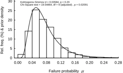
The sample size nl was chosen to be 1000. A log-normal p.d.f. π(μ | –2.71691, 0.519298) was fitted to the sample of μls as the prior density expressing the epistemic uncertainty in P(F|AS) (Figure 2). The

goodness of fit of the density π(μ) shown in Figure 2 is, strictly speaking, low. However, the ideal fit is not an end in itself. The density π(μ) merely quantifies the initial guess at P(F|AS). Therefore π(μ) can be

sub-jective to some extent (not fit ideally the simulated sample of μls).

0.00 0.04 0.08 0.12 0.16 0.20 0.24 0.28

Failure probability μ 0

5 10 15 20 25 30

Rel. freq. (%) &

prior density

Kolmogorov-Smirnov d = 0.03584, p < 0.20 Chi-Square test = 19.54864, df = 9 (adjusted) , p = 0.02091

Figure 2. Histogram of the sample {μ1, μ2, … , μ1000} and the modified lognormal prior π(μ | – 2.71691, 0.519298)×20% fitted to this sample

3.4.3. New information used for updating

The model ν(x | ξ) is only partially relevant to the

situation shown in Figure 1. It is valid for a distant free-field explosion on the ground which forms a horizontal plane. However, the tank is surrounded by a circular protective soil embankment. This will signifi-cantly influence the blast wave and reduce the ref-lected overpressure y. Thus the model ν(x | ξ) is

suffi-cient only to specify the prior density π(μ). This should be updated using new data y.

The new data y were obtained from a series of nine experiments which investigated the interaction of blast wave and circular embankment (n = 9). Elements of

the sample y are given in Table 1. This sample was transformed into the sample of f.f. values, p, by

applying the aleatory f.f. F(y | θ).

Table 1. New data y (experimental records of the overpres-sure yj) and corresponding sample of f.f. values, p

j Charge _(kg) Standoff _(m) yj (kPa) pj =F(yj|θ ) Samples obtained in experiment* Fictitious sample 1 27.0 117 3.767 1.3450089×10–4 2 26.9 142 4.276 1.0697380×10–3 3 28.2 132 4.160 6.8615251×10–4 4 31.5 125 3.944 2.8665579×10–4 5 29.3 92 4.916 9.4388105×10–3 6 33.3 50 2.920 2.1316347×10–6 7 30.0 119 4.791 6.4023419×10–3 8 34.6 86 4.032 4.1149950×10–4 9 33.0 39 2.294 5.6915293×10–8 * Data obtained by the author of this paper

3.4.4. Posterior of failure probability

The number of bootstrap replications, B, necessary

to generate the sample {μˆn′₁, μˆn′2, … , μˆn′B} was

taken to be equal to 1000. The choice of B was based

on the rules of thumb suggested in the books [36, p. 52] and [37, p. 21]. The estimate of the likelihood function, ˆL₁₀₀₀(μˆ₉|μ), was obtained by applying the Gaussian kernel function κ(.) (e.g. [37, p. 168]).

0.00 0.04 0.08 0.12 0.16 0.20 0.24 0.28

Failure probability μ

0 2 4 6 8 10 12 14 16

Densit

y _prior

likelihood posterior

Figure 3. Prior density π(μ) and the likelihood function estimate Lˆ₁₀₀₀(μˆ₉|μ) and posterior density estimate

) | (μ μ9

Situations

The approximation of the posterior density

) | (μ μ₉

πˆ ˆ was computed at the bandwidth w = 0.1.

This value was chosen using the rule w ∝B–1/3

pro-posed by Davison and Henley [37, p. 227]. The approximation πˆ(μ|μˆ₉) was obtained by a numerical calculation. The normalizing constant C(μˆ₉) found

by a numerical integration is equal to 2.99. The den-sities π(μ) and πˆ(μ|μˆ9) as well as the estimate

) | ( ₉

1000 μˆ μ

ˆL are shown in Figure 3.

4. Estimating the failure probability with the fragility function involving epistemic uncertainty

4.1. Prior density

The estimation of μ can be extended for the case of the epistemic f.f. F(y | Θ). As in the case of the

aleatory f.f. F(y), one can introduce the epistemic r.v.

∫

= =

x

X X

x x

X '

all

) ( d ) | ) | ( (

) ) | ) | ( ( (

F F

F E M

Θ Ξ ν

Θ Ξ ν

. (12)

(c)

p

1 0

m+ 1 intervals of equal width F_j(p)

pp_jj₁2

...

p p

1/(m+1)

(a)

1−F_j(p_jm)

pp_j1j2

...

f_j(p)

1

0

P(F| y)

y y_j

p

(b)

p_j1 p_jm

p_j2

...

1

0

P(F| y)

y y_j

1/(m+1)

p_jm p_jm

0 1

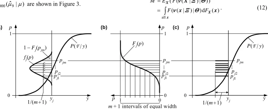
Figure 4. An approach to a discretisation of the continuous distribution of the epistemic random variable Pj

A value of M' is the failure probability correspon-ding to given values ξ and θ of Ξ and Θ. A density of

'

M can be applied as a natural prior π(μ) of μ [24].

4.2.Sample of new data

In case of the epistemic f.f. F(y | Θ), an

incorpora-tion of the new data y into updating π(μ) becomes non-trivial. The element yj of y generates an epistemic r.v.

) |

( j Θ

j F

P = y , (13)

which can be treated as imprecise observation with its own p.d.f. fj(p) and d.f. Fj(p) (Figure 4a,b). Consequently, the epistemic f.f. F(y | Θ) requires to

update π(μ) using a set of n imprecise “observations” }

, ... , , ... , ,

{P₁ P₂ Pj Pn .

An updating of the prior π(μ) with the information expressed by the r.v.s Pj is a nontrivial problem. The posterior averaging approach mentioned in Introduc-tion is not directly applicable to the present case. This approach was developed for a discrete distribution of a single uncertain datum [25, 28]. In principle, the posterior averaging could be applied by discretising the distributions of Pj in the traditional way. However, these distributions can be discretised and the prior π(μ) updated without using the posterior averaging. The heuristic principle of this discretisation is that it should yield m values pjk of Pj and these values should have equal epistemic weights wk = 1/m (k = 1, 2, …,

m). The equal weights wk assure that none of pjks will

be preferred to others. The equal wks is an analogy with the equal attitude towards elements of a sample collected by following a standard probability sampling scheme (e.g. [38, p. 106]).

The suggested principle of the discretisation is illustrated in Figure 4b,c. The values pjk can be calcu-lated by

1)) /( (

1 ₊

= −

m k F

pjk j (k = 1, 2, … , m), (14)

where −1(_⋅)

j

F is the inverse d.f. of Pj. The non-unifor-mly arranged values pjk can be interpreted as ones of a r.v. with the probability masses wk equal to 1/(m+1) (Figure 4c). The discretisation leads to a loss of the upper tail area 1 – Fj(pjm) (Figure 4a), and so wks do not strictly satisfy the condition

∑

increases.

After the transformation (14) is applied to all n

elements of the sample y, a new sample consisting of

n×m elements is obtained:

p = {(pjk, k = 1, 2, … , m), j = 1, 2, … , n}. (15) When the same number m is applied to discretise

each Pj, all elements of p will have equal epistemic weights approximately equal to 1/m. Then the sample p defined by Eq (15) can be applied in place of the

4.3. Numerical implementation and recipes

The discretisation of the continuous probability distribution of Pj distorts to a degree the information expressed by this distribution. In addition, the discreti-sation raises the question about the number m of the

discrete values pjk related to a specific yj. One can expect that the larger is m the closer is the distribution

of the probabilities pjk (k = 1, 2, … , m) to the dis-tribution of Pj (e. g., the closer is the mean pjk of the values pjk to the mean of Pj). However, the excessively large m will lead to an excessively large size n×m of

the sample p. This in turn can influence the results of

the Bayesian updating of the prior density π(μ). At present, one can say that the number m can be

chosen adaptively. Criteria for the choice of m can be

based on an interpretation of the quantities pjk (k = 1, 2, …, m) as a statistical sample which can be denoted

by

pj = {pjk, k = 1, 2, … , m}. (16)

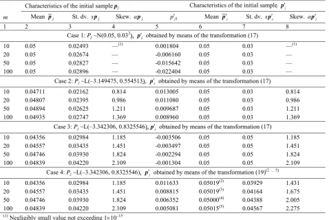
These criteria can be derived by comparing the empirical distribution of pj to the distribution of Pj. As an illustration, let us assume three distributions of Pj having the same mean and different degrees of skewness (Table 2). Each of them was discretised and four samples pj were created using the values of m = 10, 20, 50, and 100. Descriptive measures of pj are given in Cols. 2 to 4 of Table 3. It follows from this table that the difference between the mean values pj of pj and the distribution mean EPj = 0.05 increases with the increase of the distribution skewness αPj. The standard deviation spj and skewness apj of pj is smaller than the corresponding values of the probabi-lity distributions σPj and αPj (Tables 2 and 3). This, probably, is due to the loss of the upper tail area of the distribution of Pj (Figure 4a).

Table 2. Three examples of the continuous probability distribution of the epistemic random variable Pj

Distribution type Mean EPj St. dev. σPj Parameter μ Parameter σ Skewness αPj

Normal 0.05 0.03 0.05 0.03 0

Lognormal 0.05 0.03 –3.149475 0.554513 2.02*

Lognormal 0.05 0.05 –3.342306 0.8325546 4.0*

**Calculated by the formula αPj = (exp{σ

2_{}+2)( exp{σ}2_}–1)–1/2

Table 3. Descriptive measures of the initial sample pj and the adjusted sample p′j resulting from the discretisation of three prob-ability of the epistemic random variable Pj at different values of m

Characteristics of the initial sample pj Characteristics of the initial sample p′j

m Mean pj St. dv. s pj Skew. a pj p′j1 Mean p′j St. dv. s p′j Skew. a p′j

1 2 3 4 5 6 7 8

Case 1: Pj ~N(0.05, 0.032), p′j obtained by means of the transformation (17)

10 0.05 0.02493 —(1) _{0.001804 0.05 0.03 —}(1)

20 0.05 0.02674 — -0.006160 0.05 0.03 —

50 0.05 0.02827 — -0.015642 0.05 0.03 —

100 0.05 0.02896 — -0.022404 0.05 0.03 —

Case 2: Pj ~L(–3.149475, 0.554513), p′j obtained by means of the transformation (17)

10 0.04711 0.02162 0.814 0.013005 0.05 0.03 0.814

20 0.04807 0.02395 0.986 0.011080 0.05 0.03 0.986

50 0.04894 0.02625 1.211 0.009687 0.05 0.03 1.211

100 0.04935 0.02747 1.369 0.008960 0.05 0.03 1.369

Case 3: Pj ~L(–3.342306, 0.8325546),p′j obtained by means of the transformation (17)

10 0.04356 0.02984 1.185 -0.003506 0.05 0.05 1.185

20 0.04557 0.03435 1.451 -0.003497 0.05 0.05 1.451

50 0.04746 0.03930 1.824 -0.002294 0.05 0.05 1.824

100 0.04839 0.04220 2.109 -0.001304 0.05 0.05 2.109

Case 4: Pj ~L(–3.342306, 0.8325546), p′j obtained by means of the transformation (19) (2 … 5)

10 0.04356 0.02984 1.185 0.011633 0.05019(2) _{0.03929 1.431}

20 0.04557 0.03435 1.451 0.008815 0.05019(3) _{0.04164 1.675}

50 0.04746 0.03930 1.824 0.006352 0.05000(4) _{0.04388 2.005}

100 0.04839 0.04220 2.109 0.005081 0.05015(5) _{0.04567 2.275}

(1) _{Negligibly small value not exceeding 1×10}–15 (2)_Δ

j = 0.29, (3)_Δ

j = 0.22, (4)_Δ

j = 0.14, (5)_Δ

Situations

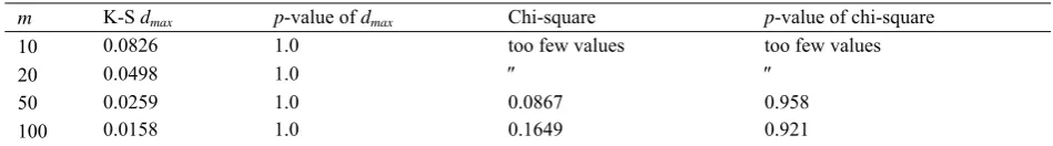
Table 4. Results of the application of the goodness-of-fit tests to the sample p′_j obtained by discretising the lognormal

distribu-tion L(– 3.149475, 0.554513)

m K-S dmax p-value of dmax Chi-square p-value of chi-square

10 0.0826 1.0 too few values too few values

20 0.0498 1.0 ″ ″

50 0.0259 1.0 0.0867 0.958

100 0.0158 1.0 0.1649 0.921

The deviation of the descriptive measures of pj from the corresponding theoretical values can be eli-minated or decreased by transforming pj. For instance, a simple linear transformation of the sample pj will not change the type of distribution of pj, namely,

j j jk j j

jk P s p EP

p′ =(σ / p )( − p )+ . (17)

Eq (17) yields an adjusted sample } , ... 1,2, ,

{pjk k k

j = ′ =

′

p , (18)

with the mean value and standard deviation precisely equal to the corresponding characteristics of Pj (Cols. 6 and 7, Table 3). At the same time, the transformation (17) leaves the skewness of pj unchanged (Cols. 4 and 7, Table 3).

The transformation (17) is applicable to both symmetrical and skewed distributions. However, it can produce negative values of p′jk, especially, in case of

small probabilities (e.g., Cases 1 and 3, Table 3). As probability is limited by the interval [0, 1], Eq (17) is applicable only to the case where p′_j1 >0 (Case 2, Table 3).

The sample pj can be adjusted to the distribution of

Pj by applying the transformation ) )/ (

1

( j jk j1 j1

jk

jk p p p p

p′ = +Δ − , (19)

where Δj is the adjustment factor, the value of which can be chosen adaptively. The transformation (19), strictly speaking, is non-linear; however, the departure from linearity is not large at small values of Δj. The transformation (19) makes the mean value p′j of the

adjusted sample p′j virtually equal to the distribution

mean EPj (Case 4, Col. 6, Table 3). At the same time, it makes standard sp′j and skewness ap′j of p′j

closer to the respective values σPj and αPj, especially in case of small values of m (Case 4, Cols. 7 and 8 in

Table 3).

The minimum value of m can be chosen by

applying goodness-of-fit tests to the samples p′j. For

instance, Table 4 shows results of applying two stan-dard tests to the sample p′j obtained by discretising

one of the lognormal distributions. One can conclude that p′j fits the lognormal distribution quite well even

at m = 10.

Further implementation problem is that the type of the probability distribution of Pj will in most cases be

unknown. However, the probability pjk following from Eq (14) is the quantile of the r.v. Pj with the level of

k/(m+1). In such a case the value pjk can be estimated by the empirical quantile pˆj,k/(m+1) computed for the sample

j

p′′ = {pj1, pj2, … , pjs, … , pjn_s}, (20)

where the sample element pjs is obtained by sampling the value θs of the parameter vector Θ from FΘ(θ) and evaluating the f.f. F(y | Θ) for the pair yj and θs:

) |

( j s

js F

p = y θ . (21)

With the sample pj′′, the empirical quantile

1) /( ,k m+

j

p

ˆ is obtained in the standard way, namely, by

ordering elements of pj′′ and choosing the element

with the number [ns×k/(m+1)]+1.

Two sets of the samples p′j and pj′′ can be

com-bined into two samples } , ... 2, 1, ,

{ ′j j= n

= ′ p

p , (22)

} , ... 2, 1, ,

{ j′′ j= n

= ′′ p

p . (23)

The fist sample p′ can be applied to updating the

prior p.d.f. π(μ) instead of the initial sample p defined

by Eq (15). The simulated sample p″ can be used to

control the quality of information represented by the sample p′ obtained by means of discretisation. It is

natural to expect that descriptive measures of p′ and p″

will be relatively close to each other.

4.4. Second example: the use of epistemic fragility function

4.4.1. Prior density of failure probability

The first example described in Sec 3.4 will now be expanded by introducing an epistemic f.f. F(y | Θ) .

This is expressed by a d.f. of a normal distribution,

F(y | Θ1,Θ2), with uncertain mean Θ1 and uncertain variance Θ2. They are assumed to be independent and distributed as indicated in Table 5. The gamma prior G(18, 14.962) of the precision 1

2−

Θ is equivalent to an inverted gamma prior IG(18, 14.962) of the variance Θ2 [39, p.20]. The unique mode of IG(18, 14.962) is 0.7875 (kPa)2 _{(e.g. [40, p.119]). This value is equal to} the “crisp” value of the corresponding f.f. parameter θ2 (Sec 3.4.1).

procedure. This generated the sample {μ1, μ2, … , μl, … ,

l n

μ }, the lth element of which, μl , is an estimate of the mean value EX(pi(ν(X|ξl)|θl)) at the given values ξl and θl = (θ1l, θ2l)T (see Eq (7)). The latter value was sampled from the distributions given in Table 5. The sample size nl was assumed to be equal to 1000.

Table 5. Prior distributions of the f.f. parameters Θ1 and Θ2* Parameter

of f.f.

Type of

prior Parameters of prior distribution

Θ1 Normal 7 kPa (mean), 0.77 kPa (sd. dev.)

1 2

−

Θ Gamma 18 (shape), 14.962 (kPa)_{1.1362 (kPa)}–2 _(mode) –2 (scale), * According to recommendations of Congdon [39, p. 19]

It was problematic to fit a widely known univariate probability distribution to the sample {μ1, μ2, … , μl, … , μ1000}. Therefore this was transformed into the

sample {–lnμ1, –lnμ2, … , –lnμ1000} and a gamma dis-tribution Ga(0.1557, 17.4929) was fitted to the latter sample (Figure 5). The transformation ψ = –lnμ was chosen intuitively. It implies that the prior π(μ) can be

obtained from the p.d.f. fΨ(ψ) of the r.v.

Ψ~Ga(α = 0.1557, β = 17.4929) using the following density transformation [41, p. 26]:

) , | (ln 1 ) ,

( μ α β

μ β α μ

π |− =− f_Ψ − , (24)

where α and β are the scale and shape parameters of the gamma distribution, respectively. The prior density π(μ) obtained using the transformation (24) is shown in Figure 6. It has a somewhat higher coefficient of variation that the prior density specified with the aleatory f.f. F(y | θ) (Sec 3.4.2).

Table 6. Descriptive measures of the samples p, p′, and p′′ used in the first and second examples

Sample size Mean Std.dev. Skewness Kurtosis Minimum Maximum 10th _{prc. 90}th _prc. The sample p obtained by applying the crisp fragility function (Table 1)

9 0.02048 5.692⋅10–8 _{1.78 2.02 5.692⋅10}–8 _6.402⋅10–3 _{—* —}

The sample p′ obtained using the discretisation with m = 50 (Eq (22))

450 0.013234 0.038145 5.2357 34.331 5.60⋅10–14 _{0.3724 2.27⋅10}–7 _0.03406 The sample p′ obtained using the discretisation with m = 100 (Eq (22))

900 0.013261 0.039008 5.5544 39.680 3.89⋅10–15 _{0.4356 1.94⋅10}–7 _0.03414 The sample p′′ obtained using the simulation (Eq (23))

900 000 0.013197 0.040145 6.3105 55.820 0.0 0.9590 — —

* Not calculated

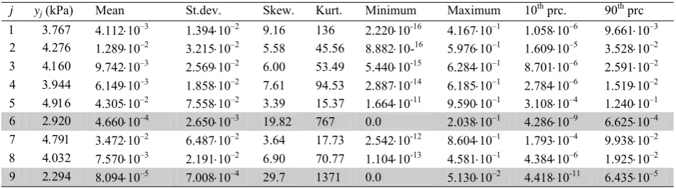
Table 7. Descriptive measures of the simulated samples pj′′ obtained with ns = 100 000 and computed for the elements yj of the initial sample y

j yj (kPa) Mean St.dev. Skew. Kurt. Minimum Maximum 10th prc. 90th prc

1 3.767 4.112⋅10–3 _1.394⋅10–2 _{9.16 136 2.220⋅10}-16 _4.167⋅10–1 _1.058⋅10–6 _9.661⋅10–3

2 4.276 1.289⋅10–2 _3.215⋅10–2 _{5.58 45.56 8.882⋅10-}16 _5.976⋅10–1 _1.609⋅10–5 _3.528⋅10–2

3 4.160 9.742⋅10–3 _2.569⋅10–2 6.00 53.49 _5.440⋅10-15 _6.284⋅10–1 _8.701⋅10–6 _2.591⋅10–2

4 3.944 6.149⋅10–3 _1.858⋅10–2 _{7.61 94.53 2.887⋅10}-14 _6.185⋅10–1 _2.784⋅10–6 _1.519⋅10–2

5 4.916 4.305⋅10–2 _7.558⋅10–2 _{3.39 15.37 1.664⋅10}-11 _9.590⋅10–1 _3.108⋅10–4 _1.240⋅10–1

6 2.920 4.660⋅10–4 _2.650⋅10–3 19.82 767 0.0 _2.038⋅10–1 _4.286⋅10–9 _6.625⋅10–4

7 4.791 3.472⋅10–2 _6.487⋅10–2 _{3.64 17.73 2.542⋅10}-12 _8.604⋅10–1 _1.793⋅10–4 _9.938⋅10–2

8 4.032 7.570⋅10–3 _2.191⋅10–2 6.90 70.77 _1.104⋅10-13 _4.581⋅10–1 _4.384⋅10–6 _1.925⋅10–2

9 2.294 8.094⋅10–5 _7.008⋅10–4 _{29.7 1371 0.0 5.130⋅10}–2 _4.418⋅10-11 _6.435⋅10–5

4.4.2. New information used for updating

The new information was represented by the sample p′ obtained by clustering the nine samples p′j

(j = 1, 2, … , 9; see Eqs (18) and (22)). The sample

j

p′ was computed by transforming the corresponding

sample pj by means of Eq (19). The linear trans-formation (17) was not applied because it produced negative elements p′jk of p′j in all nine cases. The

sample pj is a result of discretising the r.v. Pj with the

d.f. Fj(p) into a set of m quantiles pjk defined by Eq (14). As the d.f. Fj(p) is not known in the present case, the values pjk were estimated by the empirical quantiles pˆj,k/(m+1) computed for the samples pj′′,

Situations

0 1 2 3 4 5 6 7

-ln μ 0

50 100 150 200 250 300 350

N

u

mber

of

obs

er

v

a

ti

ons

Kolmogorov-Smirnov d = 0.02586, p = n.s.

Chi-Square test = 3.99308, df = 5 (adjusted) , p = 0.55041

Figure 5. Histogram of the sample {–lnμ1, –lnμ2, … , – lnμ1000} and density of the gamma distribution

Ga(0.1557, 17.4929) fitted to this sample

0.00 0.05 0.10 0.15 0.20 0.25 0.30

Failure probability μ 0

2 4 6 8 10 12 14

Pr

io

r den

s

it

y

Prior obtained with the aleatory f.f.F(y|θ) (mean of prior = 0.0756; c.o.v. of prior 55.6 %)

Prior obtained with the epistemic f.f.F(y|Θ) (mean of prior = 0.0796; c.o.v. of prior 61.5 %)

Figure 6. Lognormal prior density

π(μ | –2.71691, 0.519298) (dashed line) and transformed gamma prior density

π(μ | –0.1557, 17.4929) (solid line)

The simulated samples pj′′ were combined into the

sample p″ consisting of 900 000 elements (Eq (23)).

Descriptive measures of p″ and pj′′ are given in Tables

6 and 7, respectively.

The samples pj′′ can be used to control the results

of the discretisation expressed by the samples of quan-tiles, pj and p′j. For instance, descriptive measures of

the latter samples computed for the case m = 100 are

given in Tables 8 and 9. Descriptive measures of pj differ from the ones of pj′′ to a relatively large extend

(compare Tables 7 and 8). The transformation (19) produced the samples p′j which are closer to pj′′ in

terms of their mean values, standard deviations, and skewnesses (compare Tables 7 and 9). Larger diffe-rences in the descriptive measures were obtained only in the cases of j = 6 and j = 9, namely, in cases of a

relatively large skweness of the samples p6′′ and p9′′

(lines 6 and 9, Table 7). One can conclude that in case of highly skewed samples pj′′ the transformation (19)

should be replaced by a more sophisticated one which will yield better adjustment of the samples pj to the simulated samples pj′′.

Table 8. Descriptive measures of the samples pj obtained using the transformation (14) with m = 100

j yj (kPa) Mean St.dev. Skew. Kurt. Minimum Maximum 10th prc. 90th prc

1 3.767 3.415⋅10–3 _9.041⋅10–3 _{4.51 23.90 2.210⋅10}–9 _6.396⋅10–2 _1.026⋅10–6 _8.622⋅10–3

2 4.276 1.153⋅10–2 _2.505⋅10–2 _{3.73 16.43 7.397⋅10}–8 _1.624⋅10–1 _1.568⋅10–5 _3.203⋅10–2

3 4.160 8.606⋅10–3 _1.948⋅10–2 _{3.89 17.79 3.195⋅10}–8 _1.285⋅10–1 _8.488⋅10–6 _2.366⋅10–2

4 3.944 5.273⋅10–3 _1.309⋅10–2 _{4.28 21.57 7.107⋅10}–9 _9.057⋅10–2 _2.711⋅10–6 _1.365⋅10–2

5 4.916 4.069⋅10–2 _6.671⋅10–2 _{2.73 8.51 3.934⋅10}–6 _3.755⋅10–1 _3.054⋅10–4 _1.157⋅10–1

6 2.920 3.219⋅10–4 _1.165⋅10–3 _{5.95 40.74 1.638⋅10}-12 _9.409⋅10–3 _4.141⋅10–9 _5.742⋅10–4

7 4.791 3.258⋅10–2 _5.651⋅10–2 _{2.92 9.87 1.935⋅10}–6 _3.274⋅10–1 _1.752⋅10–4 _9.242⋅10–2

8 4.032 6.544⋅10–3 _1.572⋅10–2 _{4.11 19.85 1.347⋅10}–8 _1.064⋅10–1 _4.247⋅10–6 _1.750⋅10–2

9 2.294 4.403⋅10–5 _1.929⋅10–4 _{6.86 52.74 3.886⋅10}-15 _1.659⋅10–3 _4.219⋅10-11 _5.402⋅10–5

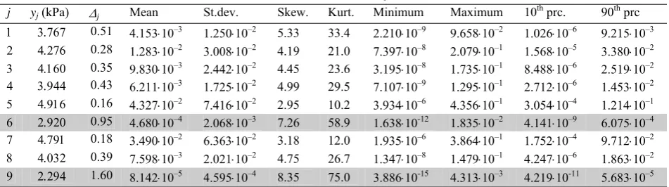
Table 9. Descriptive measures of the samples p′j obtained by transforming the samples pj by means of Eq (19) (the latter samples result from the discretisation of continuous distributions of r.v.s Pj at m = 100)

j yj (kPa) Δj Mean St.dev. Skew. Kurt. Minimum Maximum 10

th _{prc. 90}th _prc

1 3.767 0.51 4.153⋅10–3 _1.250⋅10–2 5.33 33.4 _2.210⋅10–9 _9.658⋅10–2 _1.026⋅10–6 _9.215⋅10–3

2 4.276 0.28 1.283⋅10–2 _3.008⋅10–2 _{4.19 21.0 7.397⋅10}–8 _2.079⋅10–1 _1.568⋅10–5 _3.380⋅10–2

3 4.160 0.35 9.830⋅10–3 _2.442⋅10–2 _{4.45 23.6 3.195⋅10}–8 _1.735⋅10–1 _8.488⋅10–6 _2.519⋅10–2

4 3.944 0.43 6.211⋅10–3 _1.725⋅10–2 _{4.99 29.5 7.107⋅10}–9 _1.295⋅10–1 _2.712⋅10–6 _1.453⋅10–2

5 4.916 0.16 4.327⋅10–2 _7.416⋅10–2 2.95 10.2 _3.934⋅10–6 _4.356⋅10–1 _3.054⋅10–4 _1.214⋅10–1

6 2.920 0.95 4.680⋅10–4 _2.068⋅10–3 7.26 58.9 _1.638⋅10-12 _1.835⋅10–2 _4.141⋅10–9 _6.075⋅10–4

7 4.791 0.18 3.490⋅10–2 _6.363⋅10–2 3.18 12.0 _1.935⋅10–6 _3.864⋅10–1 _1.752⋅10–4 _9.712⋅10–2

8 4.032 0.39 7.598⋅10–3 _2.021⋅10–2 _{4.75 26.7 1.347⋅10}–8 _1.479⋅10–1 _4.247⋅10–6 _1.863⋅10–2

For the case m = 100, clustering the nine samples

j

p′ resulted in a sample p′ containing 900 elements

and having descriptive measures presented in Table 6. This table contains also descriptive measures of the sample p′ obtained with m = 50 and consisting of 450

elements. Results presented in Table 6 indicate that the samples p′ are relatively close to the sample p″ as

regards their mean values, standard deviations and measures of skewness. Consequently, the samples p′

can be used for updating the prior p.d.f. π(μ).

4.4.3. Results of updating by means of Bayesian bootstrap

The samples p′ containing 450 and 900 elements

were used to calculate the respective likelihood function estimates L_B(μˆ₄₅₀|μ) and L_B(μˆ₉₀₀|μ) by

means of Eq (9). Then Eq (10) was used to obtain the approximations of posterior density, πˆ(μ|μˆ450) and

) | (μ μ₉₀₀

πˆ ˆ . The normalizing constants C(μˆ₄₅₀) and )

(μˆ900

C found by a numerical integration are equal to

3.08868 and 3.089694, respectively. As in the previous example, the number of bootstrap replications, B,

necessary to generate the sample {μˆn′1, μˆn′2, … ,

B n

μˆ′ } was taken to be equal to 1000 and the band-width w was chosen to be 0.1. Figure 7 shows the

graphs of the functions π(μ), L_B(μˆ₄₅₀|μ), and )

| (μ μ₄₅₀ πˆ ˆ .

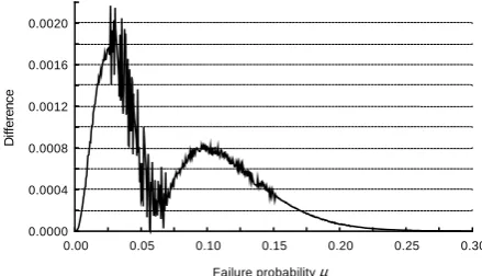
The difference between the likelihood function estimates L_B(μˆ₄₅₀|μ) and L_B(μˆ₉₀₀|μ) is slight

(Figure 8). This results in a slight difference between the posterior densities, πˆ(μ|μˆ₄₅₀) and πˆ(μ|μˆ₉₀₀)

(Figure 9). The random fluctuation of differences shown in Figures 8 and 9 is due to the application of the stochastic simulation to the sampling of bootstrap samples. The small difference between L_B(μˆ₄₅₀|μ)

and LB(μˆ900|μ) can be explained by looking at the

terms in the sum of Eq (9). The means values of the samples p′ consisting of 450 and 900 elements are

approximately equal, namely, μˆ₄₅₀ = 0.013234 and

900

μˆ = 0.013261 (Table 6). The mean values of the bootstrap samples μˆ450′ ,b and μˆ900′ ,b seem to be

relati-vely close, no matter what is the size of p′. An indirect

confirmation of this are the virtually equal mean values of the samples consisting of μˆ450′ ,b and μˆ900′ ,b:

0.0132398

1 450, 1

_∑

= − B

b b

B μˆ (st.dev. of μˆ450′ ,b=

0.00182),

0.0132397

1 900, 1

_∑

= − B

b b

B μˆ (st.dev. of μˆ900′ ,b=

0.00128). The results just mentioned allow us to conclude

that doubling the discretisation number m from 50 to

100 and so the size n×m of the sample p′ does not

tangibly influence the posterior density πˆ(μ|μˆn×m).

Thus the number m should be chosen mainly for

reasons of the best approximation of the continuous epistemic probability distribution by the sample p′.

0.00 0.05 0.10 0.15 0.20 0.25 0.30

Failure probabilityμ 0

2 4 6 8 10 12 14

De

n

s

it

y

Likelihood function estimate Prior density

Posterior densitie

Figure 7. Likelihood function estimate L(μˆ₄₅₀|μ) (solid line), prior density π(μ) (dash and line) and estimate of posterior density πˆ(μ|μˆ₄₅₀) (dotted line) obtained with the bandwidth w = 0.1

0.00 0.05 0.10 0.15 0.20 0.25 0.30

Failure probabilityμ 0.0000

0.0002 0.0004 0.0006 0.0008 0.0010 0.0012 0.0014

Dif

fe

re

n

ce

Figure 8. Values of the difference |L(μˆ450|μ)−L(μˆ900|μ)|

0.00 0.05 0.10 0.15 0.20 0.25 0.30

Failure probabilityμ 0.0000

0.0004 0.0008 0.0012 0.0016 0.0020

D

if

fe

renc

e

Figure 9. Values of the difference |πˆ(μ|μˆ450)−πˆ(μ|μˆ900)|

The approximation of the posterior density,

) | (μ μ₄₅₀

πˆ ˆ , expresses the updated epistemic

uncertainty in the failure probability P(F|AS).

Figu-re 7 indicates that πˆ(μ|μˆ₄₅₀) is more accurate that the prior density π(μ). The degree of “accuracy” can be expressed by the ranges of non-conservative and conservative percentiles given in Table 10. The new nine experimental records of the blast wave represented by the sample y decreased the uncertainty

Situations

anticipate that the conservative percentiles derived from πˆ(μ|μˆ₄₅₀)will be better understandable for the decision maker that the densities themselves. Thus the

decision concerning the potential failure event F can be made by applying these percentiles.

Table 10. Pairs of approximate percentiles derived from the prior densities π(μ) and the approximation of the posterior densities, )

| (μ μ9

πˆ ˆ and πˆ(μ|μˆ450), obtained using the crisp fragility function F(y| θ) and uncertain fragility function F(y | Θ)

Densities obtained with F(y| θ) Densities obtained with F(y| Θ)

Density characteristic _{Prior π(μ) Posterior estimate ( | )} 9

μ μ

πˆ ˆ Prior π(μ) Posterior estimate πˆ(μ|μˆ₄₅₀)

5th _{percentile 0.02813 0.0263 0.0205 0.0185}

95th _{percentile 0.1553 0.1218 0.174 0.134}

Range 0.1272 0.0955 0.1535 0.1155

1st _{percentile 0.0197 0.0186 0.0115 0.0105}

99th _{percentile 0.2012 0.1593 0.236 0.175}

Range 0.2015 0.1407 0.2245 0.1645

5. Conclusions

Estimating an imprecise failure probability by ap-plying scarce and uncertain information related to a potential failure in an abnormal situation has been considered. Two sources of information were applied to this estimating: (i) a small-size statistical sample consisting of experimental observations of characte-ristics of abnormal situation and (ii) fragility function used to express aleatory and epistemic uncertainty re-lated to the potential failure. Estimating the failure probability was formulated as a problem of Bayesian inference. Epistemic uncertainty in the failure prob-ability was expressed by means of Bayesian prior and posterior distributions. The central problem of estima-ting was Bayesian updaestima-ting with imprecise data. Such data were an intermediate result of probability estima-ting. The imprecise data were represented by a set of continuous epistemic probability distributions of the fragility function values related to elements of the small-size sample.

The Bayesian updating with the set of continuous epistemic distributions is possible by discretising these distributions. The discretisation yields a new sample which can be used for updating. This sample consists of fragility function values, each of which has equal epistemic weight. Such a discretisation can be ob-tained by dividing the range of the inverse distribution function of each epistemic distribution into equal intervals. In case where the continuous epistemic distributions are highly skewed, an additional transformation of the discrete distribution can improve the discretisation.

The proposed approach is also applicable to the case where the continuous epistemic distributions are not available in the explicit form and must be re-presented by simulated samples of fragility functions values. In this case, the discretisation can be obtained using percentiles of the simulated samples. Such a simulation will be possible for the fragility function, the values of which can be evaluated with a relatively small computational effort.

Estimating the failure probability using the sample resulting from the discretisation was illustrated by two

examples. The probability of failure due to an acciden-tal explosion was considered in these examples. The probability was estimated using a fragility function which expresses the aleatory uncertainty only and a fragility function which quantifies both aleatory and epistemic uncertainty.

References

[1] T. Aven. Perspectives on risk in a decision-making context – Review and discussion. Safety Science, Vol.

47, No.6, 2009, 798-806.

[2] E.R. Vaidogas, V. Juocevičius. Sustainable develop-ment and major industrial accidents: the beneficial role of risk-oriented structural engineering. Technological and Economic Development of Economy, Vol.14, No.4, 2008, 612-627.

[3] E.R. Vaidogas. First step towards preventing losses due to mechanical damage from abnormal actions: Knowledge-based forecasting the actions. Journal of Loss Prevention in the Process Industries, Vol.19, No.3, 2006, 375-385.

[4] E.R. Vaidogas. Explosive damage to industrial buil-dings: assessment by resampling limited experimental data on blast loading. Journal of Civil Engineering and Management, Vol.11, No.4, 2005, 251-266.

[5] E.R. Vaidogas, V. Juocevičius. Assessment of struc-tures subjected to accidental actions using crisp and uncertain fragility functions. Journal of Civil Enginee-ring and Management, Vol.15, No.1, 2009, 95-104.

[6] T. Aven, K. Pörn. Expressing and interpreting the results of quantitative risk analyses. Review and dis-cussion. Reliability Engineering & System Safety,

Vol.61, No.1, 1998, 3-10.

[7] N.D. Singpurwalla. Reliability and Risk. A Bayesian Perspective. Chichester, Wiley, 2006.

[8] E.R. Vaidogas. Handling uncertainties in structural fragility by means of the Bayesian bootstrap resamp-ling. Proceedings (CD-ROM) of Int. Conference ICASP 10, 1-3 August, 2007, Tokyo, Japan. London: Taylor & Francis, 2007.

[9] E.R. Vaidogas. Prediction of Accidental Actions Li-kely to Occur on Building Structures. An Approach Based on Stochastic Simulation, Vilnius, Technika,

[10] J. Čeponis, E. Kazanavičius, L. Čeponienė. Hand-ling multiple failures in process networks. Information Technology and Control, Vol.37, No.1, 2008, 19-25.

[11] A. Der Kiureghian. Bayesian framework for fragility assessment. Proc. of ICASP 8, ed by R.E. Melchers and M.G. Stewart. Rotterdam: Balkema, 1999,

1003-1010.

[12] B.R. Ellingwood. Earthquake risk assessment of buil-ding structures. Reliability Engineering & System Safety, Vol.74, No.3, 2001, 251-262.

[13] M. Sasani, A. Der Kiureghian, V.V. Bertero. Seis-mic fragility of short period reinforced concrete struc-tural walls under near source ground motions. Structu-ral Safety, Vol.24, No.2-4, 2002, 123-138.

[14] K.H. Lee, D.V. Rosowsky. Fragility analysis of woodframe buildings considering combined snow and earthquake loading. Structural Safety, Vol.28, No.3,

2006, 289-303.

[15] Y.Li, B.R. Ellingwood. Reliability of woodframe resi-dential construction subjected to earthquakes. Structu-ral Safety, Vol.29, No.4, 2007, 294-307.

[16] M.K. Ravindra. Extreme wind risk assessment.

Probabilistic Structural Mechanics Handbook. New York etc.: Chapman&Hall, 1995, 429-464.

[17] Y. Li, B.R. Ellingwood. Hurricane damage to residen-tial construction in the US: Importance of uncertainty modelling in risk assessment. Engineering Structures, Vol.28, No.7, 2006, 1009-1018.

[18] Th. Fetz, M. Oberguggenberger. Propagation of un-certainty through multivariate functions in the framework of sets of probability measures. Reliability Engineering & System Safety, Vol.85, No.1-3, 2004,

73-87.

[19] F. Tonon. Using random set theory to propagate epis-temic uncertainty through a mechanical system. Reli-ability Engineering & System Safety, Vol.85, No.1-3,

2004, 169-181.

[20] J.W. Hall, J. Lawry. Generation, combination and extention of random set approximations to coherent lower and upper probabilities. Reliability Engineering & System Safety, Vol.85, No.1-3, 2004, 89-101.

[21] C. Baudrit, D. Dubois, N. Perrot. Representing para-metric probabilistic models tainted with imprecision.

Fuzzy Sets and Systems, Vol.159, No.15, 2008,

1913-1928.

[22] M. Oberguggenberger, W. Fellin. Reliability bounds through random sets: Non-parametric methods and geotechnical applications. Computers & Structures, Vol.86, No.10, 2008, 1093-1101.

[23] P. Soundappan, E. Nikolaidis, R.T. Haftka, R. Grandhi, R. Canfield. Comparison of evidence theo-ry and Bayesian theotheo-ry for uncertainty modelling.

Reliability Engineering & System Safety, Vol.85, No

.1-3, 2004, 295-311.

[24] E.R. Vaidogas, V. Juocevičius. Assessment of struc-tures subjected to accidental actions using crisp and uncertain fragility functions. Journal of Civil Enginee-ring and Management, Vol.15, No.1, 2009, 95-104.

[25] N.O. Siu, D.L. Kelly. Bayesian parameter estimation in probabilistic risk assessment. Reliability Enginee-ring & System Safety, Vol.62, No.1-2, 1998, 89-116.

[26] Z. Tan, W. Xi. Bayesian analysis with consideration of data uncertainty in a specific scenario. Reliability Engineering & System Safety, Vol.79, No.1, 2003,

17-31.

[27] R. Viertl. Unvariate statistical analysis with fuzzy data. Computational Statistics & Data Analysis, Vol.

51, No.1, 2006, 133-147.

[28] D.L. Kelly, C.L. Smith. Bayesian inference in prob-abilistic risk assessment – The current state of the art.

Reliability Engineering & System Safety, Vol.94, No.2,

2009, 628-643.

[29] E.R. Vaidogas, V. Juocevičius. Reliability of a tim-ber structure exposed to fire: estimation using fragility function. Mechanika, Vol.73, No.5, 2008, 35-42.

[30] D.D. Boos, J.F. Monahan. Bootstrap methods using prior information. Biometrica, Vol.73, No.1, 1986,

77-83.

[31] J. Shao, D. Tu. The Jackknife and Bootstrap. New York etc.: Springer, 1995.

[32] R. Peek. Analysis of unanchored liquid storage tanks under lateral loads. Earthquake Engineeinrg & Sturc-tural Dynamics, Vol.16, No.7, 1988, 1087-1100.

[33] G. Landucci, G. Gubinelli, G. Antonioni, V. Cozan-ni. The assessment of the damage probability of sto-rage tanks in domino events triggered by fire. Accident analysis and Prevention, 2008 (Article in Press, doi:10.1016/j.aap.2008.05.006).

[34] E.Bareiša, V. Jusas, K. Motiejūnas, R. Šeinauskas.

The use of a software prototype for verification test generation. Information Technology and Control, Vol.

37, No.4, 2008, 265-274.

[35] V. A. Kotlerovskij et al. Shelters of Civil Defense.

Moscow, Stroijizdat, 1995. (in Russian)

[36] B. Efron, R.J. Tibshirani. An Introduction to the Bootstrap. New York: Chapman & Hall, 1993.

[37] A.C. Davison, D.V. Hinkley. Bootstrap Methods and their Application. Cambridge: Cambridge university press, 1998.

[38] V. Barnet. Sample Survey. Principles and Methods.

London etc., Edward Arnold, 1991.

[39] P. Congdon. Bayesian Statistical Modelling. Chiches-ter etc., Wiley, 2000.

[40] J.M. Bernardo, A.F.M. Smith. Bayesian Theory.

Chichester etc., Wiley, 1994.

[41] J. Kruopis. Mathematical Statistics. Vilnius, Mokslas,

1977, (in Lithuanian).