METAHEURISTIC APPROACHES FOR THE QUADRATIC MINIMUM SPANNING
TREE PROBLEM
Gintaras Palubeckis∗, Dalius Rubliauskas∗, Aleksandras Targamadz˙e∗∗ ∗Multimedia Engineering Department, Kaunas University of Technology
Studentu St. 50, LT-51368 Kaunas, Lithuania
∗∗Software Engineering Department, Kaunas University of Technology Studentu St. 50, LT-51368 Kaunas, Lithuania
e-mail: [email protected], [email protected], [email protected]
Abstract. Given an undirected graph with costs associated both with its edges and unordered pairs of edges, the quadratic minimum spanning tree problem asks to find a spanning tree that minimizes the sum of costs of all edges and pairs of edges in the tree. We present multistart simulated annealing, hybrid genetic and iterated tabu search algorithms for solving this problem. We report on computational experiments that compare these algorithms on random graphs of size up to 50 vertices. The results indicate that the iterated tabu search algorithm is superior to the other two approaches in terms of both solution quality and computation time.
Keywords:combinatorial optimization, quadratic minimum spanning tree, metaheuristics, simulated annealing, genetic algorithm, tabu search.
1. Introduction
Let G = (V, E) be an undirected graph with vertex set V and edge set E. The quadratic mini-mum spanning tree problem (QMSTP) is a general-ization of the classical minimum spanning tree prob-lem where we are given not only edge costsce >0, e ∈ E, as in the latter, but in addition also interac-tion costsceg between pairs of edgese, g,e ̸= g, in E. The quality of a spanning treeT = (V, E(T))in the case of the QMSTP is evaluated by the following objective function:
F(T) = ∑
e∈E(T)
ce+ ∑
(e,g)∈Ψ(T)
ceg, (1)
whereΨ(T)is the set of all unordered pairs of edges inE(T)(from now on we assume that the order of the subscripts does not matter, and bothceg andcge
refer to the same value). The QMSTP asks to find a spanning treeTthat minimizes the objective function given by (1). The problem was first introduced by Assad and Xu [1]. It arises in several contemporary application areas such as telecommunications, trans-portation and energy distribution.
The QMSTP can be regarded as a special case of the binary quadratic optimization problem (BQOP for short). Indeed, letS be a set of objects of some
i and byc′ij, i, j ∈ S,i < j, the cost incurred by selecting objectsiandj. Assuming thatP′is a fixed subset ofP, the BQOP can be stated as follows:
min (or max) ∑
i∈S′
c′i+ ∑
i,j∈S′,i<j
c′ij (2)
s.t. S′∈P′. (3) Perhaps the most widely studied case of (2), (3) is the one where P′ = P. This case is called an un-constrained binary quadratic optimization problem (UBQOP) (see [6], [11], [15]). As another example, for a fixed positive integerk, considerP′ consisting of all subsets ofSof sizek. Suppose that the objec-tive function in (2) is maximized. Then, for suchP′, (2), (3) is the formulation of the maximum diversity problem (see [4], [9]). The QMSTP can be recast into the form (2), (3) as well. This fact comes from the following observations:S=E;ceandcegin (1)
cor-respond to c′i andc′ij in (2), respectively; P′ is the collection of edge sets of all spanning trees ofG.
2 G. Palubeckis, D.Rubliauskas, A. Targamadz˙e
dealing with medium to large size graphs, efficient algorithms, which provide good, but not necessarily optimal solutions, are required. The first two heuris-tics for the QMSTP were given in [1]. These algo-rithms are constructive by nature and, therefore, are not able to provide good enough solutions for larger graphs. Zhou and Gen [21] presented a genetic algo-rithm (GA) in which the Prüfer number [16] to encode a spanning tree was adopted. They reported com-putational results for 17 test instances. Soak, Corne and Ahn [18] developed another genetic algorithm which employed a decoder-based redundant encod-ing strategy. They have shown that their GA imple-mentation outperforms genetic algorithm using the Prüfer number representation. More recently, Cor-done and Passeri [2] have applied a tabu search tech-nique to solve the QMSTP. At each iteration of their algorithm, the search is performed in the 1-exchange neighborhood, which consists of all spanning trees that can be obtained from the current spanning tree by replacing one of its edges with a non-tree edge. In [10], Öncan and Punnen have presented a local search algorithm with tabu thresholding. In this al-gorithm, the same neighborhood structure as in [2] is used. An artificial bee colony algorithm for solv-ing the QMSTP was proposed by Sundar and Ssolv-ingh [19]. In the last phase, the algorithm makes a call to a local search procedure. This algorithm compares favourably with earlier evolutionary approaches. Gao and Lu [5] introduced the fuzzy quadratic minimum spanning tree problem. It is formulated as expected value model, chance-constrained programming and dependent-chance programming according to differ-ent criteria. In [5], a genetic algorithm using Prüfer number representation for solving this problem was developed.
The purpose of the current paper is to investi-gate computationally the applicability of three quite different metaheuristics to the QMSTP, namely, sim-ulated annealing, genetic algorithm and tabu search. We compare two versions of the genetic algorithm. The first one is a pure GA, while the second is a GA hybridized with an effective local search procedure. The tabu search metaheuristic is represented by an it-erated tabu search algorithm. Such an approach ap-peared to be successful when applied to other combi-natorial optimization problems with quadratic objec-tive function, including the UBQOP [11], the max-imum diversity problem [12] and the Max-2-SAT problem [13], [14]. The empirical results summarized in this paper were obtained by testing the above listed algorithms on the QMSTP instances used by Cordone and Passeri [3].
The remainder of this paper is organized into five sections. In Sections 2 to 4, we describe our implementations of simulated annealing, genetic and tabu search algorithms, respectively. In Section 5, we present computational results. Finally, in Section 6, some concluding remarks are made.
To end this introduction, let us give a few no-tations used in the sequel of the paper. We denote by n andm the number of vertices and edges of a graph G = (V, E), respectively. Given a spanning tree T = (V, E(T)) of G and edges e ∈ E(T),
g ∈ E \E(T), we will write T(e, g)for the sub-graph of G obtained from T by replacing the edge
ewith the edge g. Trivially, the subgraph T(e, g)is connected if and only if it is a spanning tree. The set
N(T) = {T(e, g) | e ∈ E(T), g ∈ E\E(T)and
T(e, g)is connected} is called a neighborhood ofT. 2. Simulated annealing
In this section, we describe an implementation of the simulated annealing algorithm for solving the QMSTP. Simulated annealing (SA) is a general-purpose optimization method that attempts to exploit an analogy between the physical process of annealing and the process of obtaining a global extremum of a function. In physical annealing, a material, like metal or glass, is first heated up to a very high temperature and then slowly cooled down to reach the lowest en-ergy state. During the optimization process, each so-lution corresponds to a state of some physical system and the value of the objective function corresponds to the energy level. In our SA algorithm, the initial (high) temperature, denoted¯t, is obtained by evalu-ating a certain number of trees selected at random from the neighborhood N(T)of a randomly gener-ated spanning treeT = (V, E(T)). More precisely, suppose that the treeT′ ∈N(T)is obtained fromT
by replacing an edge e ∈ E(T)with an edge g ∈ E\E(T). We denote byδ(T, e, g) =F(T′)−F(T) the change in the objective function value when mov-ing from T to T′. Clearly, δ(T, e, g) = cg −ce+ ∑
h∈E(T)\{e}(cgh−ceh). The algorithm assigns to¯t
the largest absolute value ofδ(T, e, g)over a sample of 10000 spanning trees randomly drawn fromN(T). Other parameters of the algorithm are the cooling rate
α, minimum temperature t0, which should be very close to 0, and repetition factorR0.
ping rule, we execute the simulated annealing pro-cedure repetitively using randomly constructed span-ning trees as starting points. The steps of the main al-gorithm, named MSA (Multistart Simulated Anneal-ing), are as follows.
MSA
1. Randomly generate a spanning treeT. Initialize
T∗withT andF∗withF(T).
2. Compute¯t = max{|δ(T, e, g)| | (e, g) ∈ H}, where H is a set of randomly selected edge pairs (e, g) for which T(e, g) ∈ N(T). Set
K := ⌊(log(t0)−log(¯t))/logα⌋,R := R0n andstart:= 1.
3. Apply SA(T,T∗,F∗,t¯,K,R,α,start). Incre-mentstartby 1.
4. Check if the termination condition is satisfied. If so, then stop with the spanning treeT∗of value
F∗. Otherwise return to 3.
In the above description,T∗is used to denote the best spanning tree found so far. The corresponding value of the objective function is denoted byF∗. The algorithm starts with the treeT =T∗generated using the augmentation technique. Initially, the tree consists of a single vertex. At each ofn−1steps of the gen-eration routine, the treeT = (V(T), E(T))is aug-mented with a randomly selected edge having exactly one endpoint inV\V(T). At the end of this process, a tree spanning all the vertices inV is obtained. Step 2 of MSA prepares the parameters to be passed to the simulated annealing algorithm. The parameterK is the number of temperature reductions,Ris the num-ber of trees evaluated at a temperature level, andstart is the counter for the number of calls to the procedure SA given below.
SA(T, T∗, F∗,¯t, K, R, α,start)
1. Ifstart = 1, then initializef withF∗ (which equals F(T)). Otherwise, randomly generate a spanning treeT and setf :=F(T).
2. Initializetwith¯tandiwith 1. 3. Setj:= 1.
4. Randomly select edgeseandgsuch thatT(e, g)∈
N(T). Compute δ′ = δ(T, e, g). If δ′ 6 0, then go to 5. Otherwise, randomly draw a num-berξfrom the uniform distribution on[0,1]. If
ξ6exp(−δ′/t), then proceed to 5; else go to 6.
5. Update the treeT by substituting the edgeeby the edgeg. Setf :=f +δ′. Iff < F∗, then set
F∗ := f and storeT as the new best solution:
T∗←T.
6. Incrementjby 1. Ifj6R, then go to 4. 7. Incrementiby 1. Ifi6K, then sett:=αtand
go to 3. Otherwise return withT∗andF∗. As can be seen from the above description, sim-ulated annealing process is started from a random spanning tree. When SA is invoked for the first time, the same random tree as in MSA is used. The main body of SA consists of two nested loops. The outer one successively modifies the temperaturetby multi-plying it by the cooling factorα. The initial tempera-ture is set equal to¯t. Each iteration of the inner loop evaluates a tree selected at random from the neighbor-hoodN(T)of the current spanning treeT. If either the new tree T(e, g)is at least as good asT or the condition stated in Step 4 is satisfied, thenT(e, g)is accepted to replaceT. In the case where the current objective function valuef is smaller thanF∗, the up-dated treeTis saved as the best solution found so far. The time complexity of an iteration of the inner loop isO(m).
3. Genetic algorithm
A widely used approach for solving optimization problems is based on the idea of applying evolution-ary principles to problem solutions. The most famous technique in the area of evolutionary computation is the genetic algorithm. We have developed a GA to solve the QMSTP. In our algorithm, each individual of the population is a spanning tree represented by the list of its edges. Therefore, our approach differs from the genetic algorithm of Zhou and Gen [21], in which spanning trees are encoded using Prüfer num-bers. Our decision in choosing the tree representation was influenced by the fact that, according to several authors, including Raidl and Julstrom [17] and Got-tlieb et al. [7], the Prüfer encoding is not suitable for GA due to its low locality and heritability. More-over, Prüfer numbers can be used to represent span-ning trees only in the case where the QMSTP instance graph is complete. In this study, our aim is to develop algorithms for the QMSTP, including the genetic al-gorithm, which could deal with graphs of arbitrary density.
for-4 G. Palubeckis, D.Rubliauskas, A. Targamadz˙e
est(V, Esel) and chooses a subset of "best" candi-dates, that is, those feasible edgesefor which the sum
Qe = ce+∑g∈E
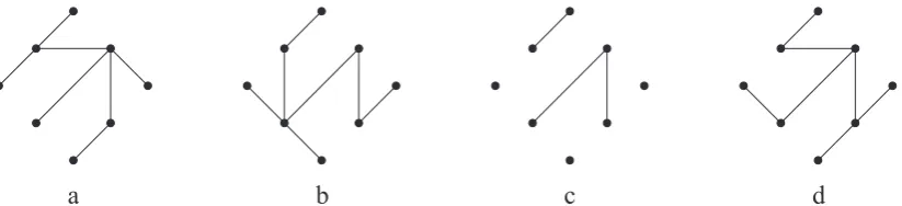
selceg is the smallest. One of the edges is randomly selected from this subset and added to the tree being built. If the resulting tree appears to be very similar to some of the individuals in the popu-lation, then it is rejected. Otherwise it is accepted as a new member of the population. Once the initial pop-ulation has been created, the algorithm enters into the evolution phase, which includes the following main steps: reproducing offspring, applying local search to offspring, and updating the current population. Let the latter be denoted byΠ. The crossover operation is performed on the two spanning trees randomly cho-sen fromΠ. It consists of two steps. In the first step, the algorithm identifies all edges that are common to both parents (for illustration, see Figure 1 where (c) displays the result of this step for parents shown in (a) and (b)). In the second step, the offspring is com-pleted by adding edges which belong to only one of the parents (Figure 1, (d)). This is done in the same way as in the above outlined randomized version of Kruskal’s algorithm. Afterwards, the offspring is sub-mitted to a local search procedure. Basically, this pro-cedure can be regarded as a kind of mutation opera-tor. To updateΠ, the algorithm employs a frequently used strategy of replacing the worst individual in the population with the generated offspring. Before do-ing this, the algorithm checks whether the offsprdo-ing is sufficiently different from each individual inΠ. If the answer is negative, then the offspring is simply discarded. The algorithm, named HGA (Hybrid Ge-netic Algorithm), can be described as follows.
HGA
1. (Initialization) SetΠ :=∅,l:= 0,F∗:=∞and
ρ:= 0. Whilel <pop_sizedo the following: 1.1. SetEsel :=∅,Ecand :=EandQe := ce
for each edgee∈E.
1.2. Form a set E′ of z = min(¯z1,|Ecand|) edgese ∈ Ecand such thatQe 6 Qg for eache ∈E′and eachg ∈ Ecand\E′ (in other words, pick thezsmallest valuesQe
among those with e ∈ Ecand). Select an edgeh∈E′at random.
1.3. Move the edge h from Ecand to Esel. If |Esel| =n−1, then proceed to 1.4. Oth-erwise, eliminate fromEcandall the edges that create a cycle when added toEsel. For the remaining edges e ∈ Ecand, increase
Qebyceh. Return to 1.2.
1.4. Ifl = 0, then go to 1.5. Otherwise, com-puteD = minT∈Π|Esel △E(T)|, where
△denotes the symmetric difference of two sets. If D > D1
min, then go to 1.5. Oth-erwise increment ρ by 1. Check whether
ρ < ρ¯. If so, then return to 1.1. If not, then setpop_size:=land escape from the loop 1.1–1.5.
1.5. Set ρ := 0. Add to Π the tree T = (V, Esel). Incrementlby 1.IfF(T)< F∗, then set T∗ := T and F∗ := F(T). If
l <pop_size, then repeat the loop. 2. (Parents selection) Randomly choose two trees,
say T1 = (V, E(T1)) and T2 = (V, E(T2)), from the populationΠ.
3. (Mating) Perform the following steps:
3.1. Initialize the setEselwith all edges that are common to both treesT1andT2.
3.2. SetEcand := E(T1)△E(T2)andQe := ce+
∑
g∈Eselceg for eache∈Ecand. 3.3. Form a set E′ of z = min(¯z2,|Ecand|)
edgese ∈ Ecand such thatQe 6 Qg for each e ∈ E′ and each g ∈ Ecand \E′. Select an edgeh∈E′at random.
3.4. Move the edge h from Ecand to Esel. If |Esel| = n−1, then go to 4. Otherwise, eliminate fromEcandall the edges that cre-ate a cycle when added toEsel. For the re-maining edgese∈ Ecand, increaseQeby
ceh. Return to 3.3.
4. (Local search) Apply the local search procedure LS(T) to the treeT = (V, Esel). LetT also de-note the tree returned by it.
5. (Offspring evaluation) Perform the following steps:
5.1. Check whetherF(T)< F∗. If so, then set
T∗:=T,F∗ :=F(T)and go to 5.3. Oth-erwise proceed to 5.2.
5.2. IfT = (V, E(T))is worse than the worst tree in the population, then go to 6. Oth-erwise, computeD = minT′∈Π|E(T)△
E(T′)|. IfD < D2min, then go to 6; else proceed to 5.3.
5.3. Replace the worst tree inΠbyT.
6. Check if the termination condition is satisfied. If so, then stop with the spanning treeT∗of value
F∗. Otherwise return to 2.
In the algorithm,pop_sizestands for the cardinal-ity ofΠ. The other parameters arez¯1,z¯2,D1min,D2min andρ¯. The first two of them are used to randomize the selection of edges during the construction of span-ning trees in the initialization and, respectively, off-spring generation steps. The role of D1minandD2min
a
b
c
d
Fig. 1. Illustration of crossover operation: (a)–(b) parents; (c) common edges; (d) offspring
is to identify those spanning trees which are too sim-ilar to at least one member of the population. Such spanning trees are not included inΠ. The parameter ¯
ρis used to stop the initialization process when it be-comes difficult to generate a diverse population of the required size. This may happen only if the graphGis very small and sparse. In the description of the algo-rithm, the best solution is denoted byT∗. Initially,T∗
is the best spanning tree in the population constructed in Step 1 of HGA. In the evolution phase,T∗ is up-dated each time a better spanning tree is found by the local search procedure LS. This procedure is an im-plementation of the 1-opt local improvement method. It goes as follows.
LS(T)
1. Initializeγ with 0. For each e ∈ E, compute
Qe = ce+∑g∈E(T)\{e}ceg, whereE(T) de-notes the edge set of the treeT as before. 2. Running through all pairs of edgese ∈ E(T)
andg ∈ E\E(T)such thatT(e, g) ∈ N(T), compute δ′ = Qg − Qe −ceg. If δ′ < 0, then perform the following actions. Exchange the edgeeinE(T)with the edgeg. Setγ:= 1,
Qe :=Qe+ceg,Qg :=Qg−ceg andQh :=
Qh−ceh+cghfor eachh∈E\ {e, g}. Go to 3. If howeverδ′>0, then repeat 2 for the next pair (e, g).
3. If γ = 0, then return with T. Otherwise, set
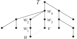
γ := 0 and go to 2 (thus, start the search for an improving exchange from the beginning). At each iteration of LS, the neighborhoodN(T) of the current treeT is explored. The algorithm tries to exchange each tree edge with each non-tree edge provided such an exchange does not create a cycle. Different ways to accomplish this are possible. Our strategy is to make the treeT rooted at any vertex and, for any edge(u, v)outsideT, using the obtained information to effectively enumerate the edges on the path fromutovinT. In order to describe this pro-cess more formally, we need a couple of notations.
For a non-root vertexi∈V, letΦibe the father ofi
in the rooted treeT. LetListand for the level of
ver-texiinT. The procedure, dubbed NS (Neighborhood Search), consists of the following two steps.
NS
1. Make the treeT rooted at any fixed vertex. 2. For each edgeg = (u, v) ∈ E \E(T)do the
following:
2.1. Initializeiwithuandjwithv.
2.2. Check whether Li > Lj. If so, then set
w := i,i := Φi ande := (i, w). If not,
then setw:=j,j:= Φjande:= (j, w).
2.3. Computeδ′for the edgeseandg. Ifi̸=j, then return to 2.2.
The described procedure is embedded in Step 2 of LS where, for each pair of edges(e, g)identified by NS, the value ofδ(T, e, g)is calculated and, depend-ing on the result, appropriate actions are taken. The behavior of NS is illustrated in Figure 2 where(u, v) is the edge to be added toT. Notice that the order of assignment statements in Step 2.2 of NS is fixed. It is not hard to see that Step 1 of NS (i.e., getting Φi
andLi for non-root vertices i ∈ V) requiresO(n)
time. The complexity of Step 2 of NS isO(nm). In the case of dense graphs, it amounts toO(n3). Thus the time of making the tree rooted is negligible com-pared with the overall time taken by NS. As it can be seen from the description of LS, exploration of the neighborhood is restarted after each update of the cur-rent spanning tree. This means that a new rooted tree needs to be built (or the existing one reconfigured). However, as just remarked, this operation is compu-tationally very cheap.
In closing this section, we note that the pure ge-netic algorithm can be obtained simply by removing Step 4 from HGA. Moreover, to keep a higher level of intensification in the search process it is useful to make the selection of an edge in Step 3.3 determin-istic. The modification is to choose an edge with the
6 G. Palubeckis, D.Rubliauskas, A. Targamadz˙e
v
w
w
w
u
w
3 4
1 2
T
Fig. 2. Illustration for Step 2 of LS: the edges for removal fromT are considered in the order
(u, w1),(w1, w2),(v, w3),(w2, w4),
(w3, w4)
smallest value ofQe. This can be done by settingz¯2 to 1 in Step 3.3 of HGA.
4. Iterated tabu search
At the core of our third algorithm is an adapta-tion of the tabu search technique to the quadratic min-imum spanning tree problem. In order to obtain better solutions, we apply the tabu search procedure repeat-edly. To get a starting spanning tree for the next itera-tion, a solution perturbation mechanism is used. The main procedure of the iterated tabu search algorithm can be stated as follows.
ITS
1. Randomly generate a spanning treeT = (V, E(T)). InitializeT∗withTandF∗withF(T). For each
e∈E, computeQe=ce+ ∑
g∈E(T)\{e}ceg.
2. Randomly draw an integerI betweenImin and
Imax. Execute the tabu search procedure TS(T,
T∗,F∗,I).
3. Check if the termination condition is satisfied. If so, then go to 5. Otherwise proceed to 4. 4. Randomly draw integers p¯ andq¯in {a1, a1 +
1, . . . , a2}and{b1, b1+1, . . . , b2}, respectively; herea1,b1 andb2are constants, whereasa2 is an integer chosen at random from the interval [nλ1, nλ2]. Apply GST(T,p¯,q¯). Return to 2. 5. Stop with the spanning treeT∗of valueF∗.
In Step 1 of ITS, an initial spanning tree is gener-ated. For this purpose, the same algorithm as in MSA is used. This step also initializes the variables Qe,
e ∈ E. They are needed to efficiently compute the decrease (or increase) in the objective function value that will result from exchanging an edge inE(T)with an edge inE\E(T). Step 2 of ITS invokes the tabu search procedure TS. The input to TS includes the number of iterations for a tabu search run, denoted by
I. This number is taken from the interval[Imin, Imax], whereIminandImaxare the parameters of ITS. Other
parameters are used in Step 4 to get the values of ¯
pandq¯. These values are submitted to the solution perturbation procedure, named GST (Get Start Tree). We shall discuss the meaning ofp¯andq¯later in this section. Making I,p¯andq¯variable strengthens the search diversification capabilities of the algorithm.
Next, we will present the main ingredients of ITS, namely, TS and GST. In the description of TS given below,τe,e ∈ E, are the tabu values and¯τis
the tabu tenure, which in our experiments was set to min(10, m/4).
TS(T, T∗, F∗, I)
1. Initializeiandτe,e∈E, with 0. Setf :=F(T). 2. Incrementiby 1. Setδ∗:=∞andµ:= 0. 3. Running through all pairs of edgese ∈ E(T)
andg ∈ E\E(T)such thatT(e, g) ∈ N(T), perform the following steps.
3.1. Computeδ′ =Qg−Qe−ceg. Ifδ′> δ∗, then go to 3.3. Otherwise check whether
f +δ′ < F∗. If so, then setδ∗ := δ′,
h := e, d := g,µ := 1and go to 4. If not, then proceed to 3.2.
3.2. If at least one ofτe,τgis positive, then go to 3.3. Otherwise check whetherδ′ < δ∗. If so, then setδ∗:=δ′,h:=e,d:=gand
k := 1. If not, then incrementkby 1 and seth:=e,d:=gwith probability1/k. 3.3. Repeat 3.1 and 3.2 for the next pair(e, g),
if any.
4. Exchange the edgehinE(T)with the edged. Setf :=f+δ∗. UpdateQe,e∈E(in the same way as it is done in Step 2 of the LS procedure). Ifµ= 1, then go to 5. Otherwise go to 6. 5. Apply the local search procedure LS to the tree
T. LetT also denote the tree returned by it. Set
T∗:=T,F∗:=F(T)andf :=F∗.
6. Ifi=I, then return. Otherwise, decrement each positiveτe,e ∈ E, by 1, setτh := ¯τ,τd := ¯τ
and go to 2.
As can be seen, TS consists of the initializa-tion part and the loop comprising Steps 2–6, which is generally executed I times. It is, however, possi-ble to terminate TS prematurely in Step 6 after the time allotted for the ITS run has expired. The most costly part of TS is Step 3 where the neighborhood of the current spanning treeTis explored. Like in the LS case, this is done using the procedure NS. For a treeT(e, g)obtained while running NS, the condition
F(T(e, g)) = f +δ(T, e, g)< F∗is checked. If it is satisfied, then the indicatorµis set to 1. Obviously, G. Palubeckis, D. Rubliauskas, A. Targamadzė
µ= 1means that a new best solution in the ITS run has been found. Only in this case the local search pro-cedure is applied. It is essentially the same as LS used in HGA. The only difference is that now the initial-ization ofQe,e∈E, in Step 1 of LS is not required.
Indeed, the values ofQeare computed in Step 1 of ITS and are maintained by both TS and GST.
The tabu search is restarted from a spanning tree produced by the procedure GST implementing a strat-egy for perturbation of the current spanning treeT. Besides T, the input to GST includes parameters p¯ andq¯. The parameterp¯is the number of edges to be removed fromT. The procedure is randomized. An edge for removal and a non-tree edge replacing it are picked at random from the candidate list of length at mostq¯. This list is constructed by including edge pairs (e, g)of type (tree edge, non-tree edge) for which the valuesδ(T, e, g)are smallest. An additional require-ment is that each edge can be chosen (to remove from
T or to add toT) at most once. The perturbation al-gorithm proceeds as follows.
GST(T,p,¯q¯) 1. Setp:= 0andE˜:=∅.
2. If B := {(e1, e2) | e1 ∈ E(T) \ E, e˜ 2 ∈
E\(E(T)∪E˜), T(e1, e2)∈N(T)}is empty, then return. Otherwise, form a set B′ of q = min(¯q,|B|) edge pairs(e1, e2) ∈ B such that
δ(T, e1, e2) 6 δ(T, g1, g2) for each(e1, e2) ∈
B′and each(g1, g2)∈B\B′. Randomly select (h1, h2)∈B′.
3. Exchange the edgeh1inE(T)with the edgeh2. Addh1andh2toE˜. UpdateQe,e∈E. 4. Incrementpby 1. Ifp <p¯, then go to 2.
Other-wise return.
In Step 2 of GST, the setB is searched in order to retrieve edge pairs with the smallestδvalues. For this purpose, we again use the procedure NS stated in the previous section.
5. Experimental results
In this section, we present some computational results in order to evaluate the performance of the al-gorithms we have described. All the alal-gorithms have been coded in the C programming language and all the tests have been carried out on a PC with an Intel Core 2 Duo CPU running at 3.0GHz. The sources are publicly available at http:
//www.soften.ktu.lt/˜gintaras/qmstp.html. As a testbed for the algorithms, the problem instances introduced by Cordone and Passeri [3] were considered. We will
provide results only for the largest instances in their test set. More specifically, in the main experiments, we used graphs ranging in size from 40 to 50 vertices. To compare HGA with the pure genetic algo-rithm, we performed tests also on a few of the graphs of order 30 and 35. The density of each graph in the testbed is one of the following:33%,67%and100%. Based on the results of preliminary computa-tional experiments with algorithms, we have fixed the values of their parameters: for MSA,α = 0.95,
t0 = 0.0001,R0 = 100; for HGA,pop_size=100, ¯
z1= 20,z¯2= 10,D1min=D 2
min= 6,ρ¯= 1000; for ITS,a1= 10,λ1 = 0.1,λ2 = 1,b1 = 5,b2= 300,
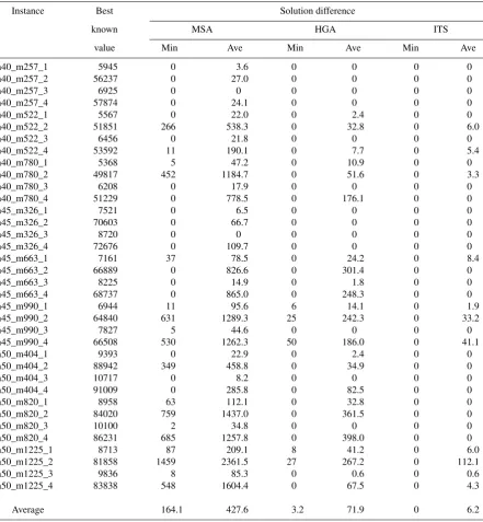
Imin = 100,Imax = 200. For the pure genetic algo-rithm, the same values as in the case of HGA were used, except that the parameterz¯2was fixed at 1. The results presented in this section were obtained by per-forming 10 runs of each algorithm on each problem instance in the test set. In the first experiment, the cut-off time for each run was 10 seconds. The results of MSA, HGA and ITS are summarized in Tables 1 and 2. The first column of these and subsequent tables represents the problem instances. In the name of an instance, the integer following "n" indicates the graph order (the number of its vertices), whereas the integer following "m" shows the number of its edges. For ex-ample, n40_m257_1 denotes the first instance whose graph has 40 vertices and 257 edges. The second col-umn of Table 1 gives the best objective function val-ues, which were reported by Cordone and Passeri [3]. The third (respectively, fourth) column shows the dif-ference between the value of the best solution out of 10 runs (respectively, the average value of 10 solu-tions) found by MSA and the value displayed in the second column. The rest of Table 1 gives these differ-ences for HGA and ITS. Table 2 includes the results for the 24 largest instances only. The second and third columns of this table, for each instance, provide the shortest (out of 10 runs) and, respectively, the aver-age CPU time taken by MSA to first find a solution that is best in the run. The remaining columns report the CPU time taken by HGA and ITS. The results, av-eraged over all tested instances, are presented in the last row of each table.
8 G. Palubeckis, D.Rubliauskas, A. Targamadz˙e
Table 1. Results of running MSA, HGA and ITS on the chosen dataset (time limit=10s)
Instance Best Solution difference
known MSA HGA ITS
value Min Ave Min Ave Min Ave
n40_m257_1 5945 0 3.6 0 0 0 0
n40_m257_2 56237 0 27.0 0 0 0 0
n40_m257_3 6925 0 0 0 0 0 0
n40_m257_4 57874 0 24.1 0 0 0 0
n40_m522_1 5567 0 22.0 0 2.4 0 0
n40_m522_2 51851 266 538.3 0 32.8 0 6.0
n40_m522_3 6456 0 21.8 0 0 0 0
n40_m522_4 53592 11 190.1 0 7.7 0 5.4
n40_m780_1 5368 5 47.2 0 10.9 0 0
n40_m780_2 49817 452 1184.7 0 51.6 0 3.3
n40_m780_3 6208 0 17.9 0 0 0 0
n40_m780_4 51229 0 778.5 0 176.1 0 0
n45_m326_1 7521 0 6.5 0 0 0 0
n45_m326_2 70603 0 66.7 0 0 0 0
n45_m326_3 8720 0 0 0 0 0 0
n45_m326_4 72676 0 109.7 0 0 0 0
n45_m663_1 7161 37 78.5 0 24.2 0 8.4
n45_m663_2 66889 0 826.6 0 301.4 0 0
n45_m663_3 8225 0 14.9 0 1.8 0 0
n45_m663_4 68737 0 865.0 0 248.3 0 0
n45_m990_1 6944 11 95.6 6 14.1 0 1.9
n45_m990_2 64840 631 1289.3 25 242.3 0 33.2
n45_m990_3 7827 5 44.6 0 0 0 0
n45_m990_4 66508 530 1262.3 50 186.0 0 41.1
n50_m404_1 9393 0 22.9 0 2.4 0 0
n50_m404_2 88942 349 458.8 0 34.9 0 0
n50_m404_3 10717 0 8.2 0 0 0 0
n50_m404_4 91009 0 285.8 0 82.5 0 0
n50_m820_1 8958 63 112.1 0 32.8 0 0
n50_m820_2 84020 759 1437.0 0 361.5 0 0
n50_m820_3 10100 2 34.8 0 0 0 0
n50_m820_4 86231 685 1257.8 0 398.0 0 0
n50_m1225_1 8713 87 209.1 8 41.2 0 6.0
n50_m1225_2 81858 1459 2361.5 27 267.2 0 112.1
n50_m1225_3 9836 8 85.3 0 0.6 0 0.6
n50_m1225_4 83838 548 1604.4 0 67.5 0 4.3
Average 164.1 427.6 3.2 71.9 0 6.2
MSA. In all cases, the average values ofF obtained by HGA are smaller than or equal to those obtained using MSA. Thus, HGA is the second best algorithm in our tests.
From Table 2, we see that, considering the CPU time required by the algorithms to find the best so-lution in the run, HGA is comparable to ITS. These algorithms are significantly faster than MSA.
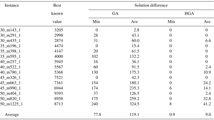
In Table 3, we compare the performance of the pure genetic algorithm, denoted as GA, with that of
Table 2. Time to the best solution in the run for graphs of order 45 and 50 (in seconds)
Instance MSA HGA ITS
Max Ave Max Ave Max Ave
n45_m326_1 9.0 4.3 0.3 0.2 0.2 0.1
n45_m326_2 7.2 1.7 0.3 0.2 0.5 0.2
n45_m326_3 3.6 1.0 0.4 0.2 <0.1 <0.1
n45_m326_4 7.5 3.0 1.1 0.5 1.0 0.4
n45_m663_1 6.4 3.3 8.1 2.8 9.1 4.0
n45_m663_2 7.3 3.7 9.2 2.8 1.9 0.6
n45_m663_3 6.2 3.3 5.5 2.7 0.6 0.2
n45_m663_4 7.1 6.4 5.0 2.8 1.8 0.7
n45_m990_1 9.6 4.9 8.2 2.5 9.3 3.9
n45_m990_2 10.0 6.7 8.2 3.4 7.1 2.3
n45_m990_3 9.4 7.0 0.6 0.4 0.9 0.4
n45_m990_4 9.8 5.1 9.2 3.2 9.7 5.2
n50_m404_1 4.7 2.0 4.5 0.8 0.7 0.2
n50_m404_2 9.6 4.5 5.3 1.9 0.5 0.2
n50_m404_3 8.6 4.3 0.1 0.1 0.2 <0.1
n50_m404_4 9.7 4.7 0.9 0.3 0.9 0.2
n50_m820_1 8.6 3.8 7.0 2.7 8.4 2.2
n50_m820_2 9.5 6.3 9.9 4.2 7.9 3.7
n50_m820_3 8.7 4.6 0.5 0.3 0.3 0.2
n50_m820_4 9.5 6.4 7.6 2.9 7.2 2.0
n50_m1225_1 3.1 2.8 8.0 3.6 9.4 5.0
n50_m1225_2 3.3 2.8 8.7 4.5 9.8 5.1
n50_m1225_3 3.5 3.0 9.0 4.3 8.2 3.9
n50_m1225_4 3.0 2.7 3.7 1.9 8.5 4.4
Average 7.3 4.1 5.1 2.0 4.3 1.9
Table 3. Comparison of GA and HGA (time limit=10s)
Instance Best Solution difference
known GA HGA
value Min Ave Min Ave
n30_m143_1 3205 0 2.8 0 0
n30_m291_1 2998 28 43.1 0 0
n30_m435_1 2874 31 60.0 0 6.6
n35_m196_1 4474 0 15.4 0 0
n35_m398_1 4147 20 61.5 0 0
n35_m595_1 4000 102 132.2 0 0
n40_m257_1 5945 16 36.1 0 0
n40_m522_1 5567 60 91.5 0 2.4
n40_m780_1 5368 130 175.3 0 10.9
n45_m326_1 7521 0 42.3 0 0
n45_m663_1 7161 154 180.1 0 24.2
n45_m990_1 6944 174 235.3 6 14.1
n50_m404_1 9393 37 126.5 0 2.4
n50_m820_1 8958 175 259.2 0 32.8
n50_m1225_1 8713 240 324.5 8 41.2
10 G. Palubeckis, D.Rubliauskas, A. Targamadz˙e
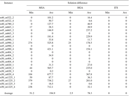
Table 4. Results of longer runs of MSA, HGA and ITS (time limit=180s)
Instance Solution difference
MSA HGA ITS
Min Ave Min Ave Min Ave
n40_m522_2 0 101.2 0 16.4 0 0
n40_m522_4 11 50.7 0 6.6 0 0
n40_m780_2 0 127.7 0 46.9 0 0
n45_m663_1 17 28.3 0 20.9 0 0
n45_m663_2 0 146.9 0 237.2 0 0
n45_m663_3 0 0 0 0 0 0
n45_m663_4 0 181.4 0 229.9 0 0
n45_m990_1 1 33.8 6 11.7 0 0
n45_m990_2 274 525.8 25 178.5 0 0
n45_m990_3 0 0 0 0 0 0
n45_m990_4 50 421.1 0 154.1 0 0
n50_m404_1 0 0 0 0 0 0
n50_m404_2 0 34.9 0 0 0 0
n50_m404_3 0 0 0 0 0 0
n50_m404_4 0 0 0 0 0 0
n50_m820_1 0 31.3 0 27.0 0 0
n50_m820_2 44 565.7 0 235.0 0 0
n50_m820_3 0 0.2 0 0 0 0
n50_m820_4 104 677.7 0 367.8 0 0
n50_m1225_1 59 87.7 0 36.3 0 0
n50_m1225_2 379 738.2 27 201.0 0 0
n50_m1225_3 0 18.5 0 0.6 0 0
n50_m1225_4 238 712.1 0 32.1 0 0
Average 51.2 194.9 2.5 78.3 0 0
(Min= 0,Ave= 994.6for GA) instances.
In our second experiment, we allowed the algo-rithms to run longer. We have limited the computation time to 3 minutes (180 seconds) per run. We tested MSA, HGA and ITS on all instances of size 50 as well as on 8 densest instances of size 45 and 3 in-stances of size 40 for which ITS failed to find the best solutions in at least one of the 10-second runs. The results are summarized in Tables 4 and 5. As Table 4 shows, ITS again outperforms HGA and again HGA is ranked ahead of MSA. We can notice that ITS suc-ceeded in finding the best solutions in all the runs. Meanwhile, the HGA implementation was still unable to reach the best known minima for 3 instances. In ad-dition, the average performance of HGA in a number of test cases was not good enough. It can be observed that the difference between the quality of solutions produced by HGA and those produced by MSA be-comes smaller as the amount of time allotted for each run of the algorithm increases. As seen in Table 4, MSA performed better than HGA for n45_m663_2 and n45_m663_4 and was not dominated by HGA in
the case of the n45_m990_1 instance.
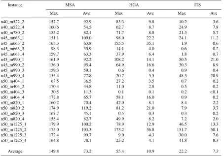
The results in Table 5 indicate that the CPU time taken to find the best solution is smaller for ITS than for the other two approaches. In fact, a time limit of 60 seconds was sufficient for ITS to deliver the best spanning trees in all the runs for each benchmark in-stance except n50_m1225_2. Again, as in the first ex-periment, MSA is the slowest of the examined algo-rithms.
6. Conclusions
Table 5. Time to the best solution in the run (in seconds)
Instance MSA HGA ITS
Max Ave Max Ave Max Ave
n40_m522_2 152.7 92.9 83.3 9.8 10.2 3.6
n40_m522_4 160.6 54.5 62.7 8.7 24.9 7.8
n40_m780_2 155.2 82.1 71.7 8.8 21.3 5.7
n45_m663_1 151.1 109.0 98.0 22.2 24.1 11.2
n45_m663_2 163.3 63.8 155.5 35.1 1.9 0.6
n45_m663_3 98.3 35.9 14.1 4.0 0.6 0.2
n45_m663_4 159.7 63.3 37.9 6.4 1.8 0.7
n45_m990_1 161.9 92.2 108.2 14.1 50.5 21.0
n45_m990_2 136.0 95.4 64.9 16.6 30.3 8.9
n45_m990_3 159.3 59.1 0.6 0.4 0.9 0.4
n45_m990_4 155.4 77.8 20.7 5.5 48.3 20.9
n50_m404_1 67.5 36.5 27.2 3.5 0.7 0.2
n50_m404_2 170.4 44.8 11.0 2.8 0.5 0.2
n50_m404_3 30.5 11.3 0.1 0.1 0.2 <0.1
n50_m404_4 172.8 65.7 58.1 16.0 0.9 0.2
n50_m820_1 160.2 70.4 42.0 8.1 8.4 2.2
n50_m820_2 174.9 119.2 81.2 21.0 7.9 3.7
n50_m820_3 167.7 45.1 0.5 0.3 0.3 0.2
n50_m820_4 155.4 82.7 49.9 8.2 7.2 2.0
n50_m1225_1 179.9 100.2 78.9 12.9 46.5 13.3
n50_m1225_2 175.0 103.3 173.2 36.8 151.7 50.1
n50_m1225_3 172.4 99.7 9.0 4.3 30.0 7.6
n50_m1225_4 164.8 78.1 25.2 4.1 41.8 8.3
Average 149.8 73.2 55.4 10.9 22.2 7.3
periments. However, the success of HGA strongly de-pends on the use of a local search procedure. The ge-netic algorithm without local search performed rather poorly. This version of GA is not competitive with the other algorithms (MSA, HGA and ITS) involved in the comparison. On the basis of our results, it may be speculated that also other approaches incorporat-ing local search could be promisincorporat-ing techniques for the QMSTP. Such approaches include VNS (Vari-able Neighborhood Search) and GRASP (Greedy Randomized Adaptive Search Procedure) with path-relinking.
References
[1] A. Assad, W. Xu. The quadratic minimum span-ning tree problem. Naval Research Logistics, 1992,
Vol.39, 399–417.
[2] R. Cordone, G. Passeri. Heuristic and exact ap-proaches to the quadratic minimum spanning tree problem. In: Seventh Cologne–Twente Workshop on Graphs and Combinatorial Optimization (CTW08), May 13–15, 2008, Gargnano, Italy, Università degli
Studi di Milano, 2008, pp. 52–55.
[3] R. Cordone, G. Passeri. The quadratic minimum spanning tree problem (QMSTP). http://homes.dsi.unimi.it/˜cordone/research/qmst.html. Accessed 27 October 2010
[4] A. Duarte, R. Martí. Tabu search and GRASP for the maximum diversity problem. European Journal
of Operational Research, 2007,Vol.178, 71–84.
[5] J. Gao, M. Lu. Fuzzy quadratic minimum spanning tree problem.Applied Mathematics and Computation, 2005,Vol.164, 773–788.
[6] F. Glover, Z. Lü, J.-K. Hao. Diversification-driven tabu search for unconstrained binary quadratic prob-lems. 4OR–A Quarterly Journal of Operations
Re-search, 2010,Vol.8, 239–253.
[7] J. Gottlieb, B.A. Julstrom, G.R. Raidl, F. Roth-lauf. Prüfer numbers: a poor representation of span-ning trees for evolutionary search. In: Proceedings of the Genetic and Evolutionary Computation Con-ference, San Francisco, CA, USA, Morgan Kaufmann
Publishers, 2001, pp. 343–350.
[8] J.B. Kruskal. On the shortest spanning subtree of a graph and the traveling salesman problem.
Proceed-ings of the American Mathematical Society, 1956,
Vol.7, 48–50.
[9] R. Martí, M. Gallego, A. Duarte. A branch and
12 G. Palubeckis, D.Rubliauskas, A. Targamadz˙e
bound algorithm for the maximum diversity
prob-lem. European Journal of Operational Research,
2010,Vol.200, 36–44.
[10] T. Öncan, A.P. Punnen. The quadratic minimum spanning tree problem: a lower bounding procedure and an efficient search algorithm.Computers and
Op-erations Research, 2010,Vol.37, 1762–1773.
[11] G. Palubeckis. Iterated tabu search for the uncon-strained binary quadratic optimization problem.
In-formatica, 2006,Vol.17, 279–296.
[12] G. Palubeckis. Iterated tabu search for the maximum diversity problem.Applied Mathematics and
Compu-tation, 2007,Vol.189, 371–383.
[13] G. Palubeckis. Solving the weighted Max-2-SAT problem with iterated tabu search. Information
Tech-nology and Control, 2008,Vol.37, 275–284.
[14] G. Palubeckis. A new bounding procedure and an improved exact algorithm for the Max-2-SAT
prob-lem. Applied Mathematics and Computation, 2009,
Vol.215, 1106–1117.
[15] P.M. Pardalos O.A. Prokopyev, O.V. Shylo, V.P. Shylo. Global equilibrium search applied to the unconstrained binary quadratic optimization
prob-lem. Optimization Methods and Software, 2008,
Vol.23, 129–140.
[16] H. Prüfer. Neuer beweis eines satzes über permu-tationen. Archiv für Mathematik und Physik, 1918,
Vol.27, 742–744.
[17] G.R. Raidl, B.A. Julstrom. Edge sets: an effective evolutionary coding of spanning trees.IEEE
Transac-tions on Evolutionary Computation, 2003,Vol.7, 225–
239.
[18] S.-M. Soak, D.W. Corne, B.-H. Ahn. The edge-window-decoder representation for tree-based prob-lems. IEEE Transactions on Evolutionary Computa-tion, 2006,Vol.10, 124–144.
[19] S. Sundar, A. Singh. A swarm intelligence approach to the quadratic minimum spanning tree problem.
In-formation Sciences, 2010,Vol.180, 3182–3191.
[20] W. Xu. On the quadratic minimum spanning tree problem. In: M. Gen, W. Xu (Eds.), Proceedings of 1995 Japan–China International Workshops on
Infor-mation Systems, Ashikaga, Japan, 1995, pp. 141–148.
[21] G. Zhou, M. Gen. An effective genetic algorithm ap-proach to the quadratic minimum spanning tree
prob-lem. Computers and Operations Research, 1998,
Vol.25, 229–237.
G. Palubeckis, D. Rubliauskas, A. Targamadzė