Algebraic Approach for Analysis and Control of a Water Tank System
Juri Belikov, Ülle Kotta
Institute of Cybernetics at Tallinn University of Technology, Akadeemia tee 21, 12618 Tallinn, Estonia,
e-mail: jbelikov@cc.ioc.ee, kotta@cc.ioc.ee
Aleksei Tepljakov
Department of Computer Control, Tallinn University of Technology, Ehitajate tee 5, 19086 Tallinn, Estonia,
e-mail: aleksei.tepljakov@ttu.ee
http://dx.doi.org/10.5755/j01.itc.45.2.13212
Abstract. Modern nonlinear control theory provides various powerful frameworks. Some of them are still either out of sight of the industry or too complex to be implemented. In this paper, we present and explain the key points of an algebraic framework of differential forms. Together with Mathematica based software package NLControl it forms a powerful basis toward the employment in analysis and control of various complex processes. The application is illustrated on the basis of the laboratory model of three serially connected water tanks, and comparison with the results obtained by using classical PID controller is presented.
Keywords: nonlinear control systems; algebraic methods; water tank system.
1. Introduction
Mathematical theory has formed a basis for imple-mentation of complex methods in industrial applica-tions. Though classical control techniques (such as PID controllers) are popular and widely used [1] in spite of existing drawbacks, the majority of automa-tion manufacturers realize the potential of advanced control techniques. These methods offer a compre-hensive analysis and more efficient control. At the same time they require specific knowledge and certain skills for the maintenance of corresponding control systems.
In this paper, we explain key points and expose the potential of the algebraic framework of differential forms. The key idea of the framework is working with differentials of system equations rather than with equations themselves. Then, vector spaces of differen-tial forms over suitable differendifferen-tial fields of nonlinear functions may be constructed [2]. Thus, the remaining part of the analysis is very similar to that of the linear case except that coefficients of the basis elements are now meromorphic functions in independent system variables and not numbers as in the linear case. The benefit of such a framework is that it suggests a wide range of rigorous mathematical tools and a systematic
way to handle different control problems from a unified viewpoint. The approach has been successfully applied so far to address a number of problems for nonlinear control systems, including system reduction [3], realization [4] of i/o differential or difference equations, accessibility and feedback linearization of state equations [2]. On one hand, the algebraic approach requires a lot of mathematical technicalities to be used to perform analysis and obtain a solution, making this way an artificial gap between theory and practice. On the other hand, it is more transparent (intuitively understandable) than, for example, the most popular differential geometrical methods [2]. Moreover, it suggests generic (that holds almost everywhere except on a set of measure zero) solution of the problem and not a local solution like most of the other approaches. This paper is intended to demonstrate and explain the difficult key aspects of the algebraic approach.
[6]. Common examples of industrial applications include chemical engineering, wastewater treatment, breweries, refineries and food processing [7] as well as different irrigation systems like dams, etc. Through the years, various techniques have been used to control the process. In many cases PID [7] or fractional-order PID [8] controllers provide acceptable solution. While such controllers are still popular choice in many industrial applications, they do not guarantee that system will work with the same level of accuracy in the entire operating range. Thus, more advanced control techniques can be used to increase the quality of control algorithms.
The rest of the paper is organized as follows. In Section 2 a brief exposition of the algebraic frame-work and the solution of the exact feedback lineariza-tion problem are presented. Next seclineariza-tion serves as a brief introduction to the software package for symb-olic computations—NLControl. Section 4 describes a mathematical model of the water tank system, accom-panied by explanatory comments. Next, precise analy-sis and controller syntheanaly-sis, using the algebraic forma-lism, are provided. Several possible configurations are presented together with experimental results. Conclu-ding remarks are given in the last section.
2. Algebraic framework
Note that throughout the paper we use the notation ( )
: d ( ) / d
k k k
t t
for the k th-order time derivative of the variable
. Sometimes, we also use notations: d ( ) / d ,t t
2 2: d ( ) / d .t t
In addition, for notational convenience, denote ( )
( ) ( )
: , ,
i n i k
for 0 i n, ik, where (0) stands for
.Consider a nonlinear multi-input multi-output (MIMO) continuous-time system, described by the state equations
, , x f x u y h x
(1)
where ( ) n
x t is the vector of state variables, ( ) m
u t is the vector of input signals, y p is the
vector of output signals, f and h are meromorphic functions.
Below we briefly recall the algebraic formalism, focused on generic system properties that hold on open and dense subsets of suitable domains of definition, provided that they hold at some points of such domains. The generic approach motivates the choice of meromorphic functions in the system description (1), see [2] for more details. Let denote the field of meromorphic functions in a finite number of independent system variables from the infinite set
, 1, , ; ( )k , 1, , , 0
i j
x i n u j m k
.
Define the time derivative operator d / d :t
as
( ) ( 1)
(0 ) 1 ( ) ( ) 1 0 d d , , , d d d d d . , d d d k k j j n k i i i m k j k
j k j
x f x u u u
t t
x u x
t x t
u t u
Observe that the field is defined by the system equations (1) since the application of the operator
d / dt to x results in x which, according to (1), is not an independent variable and has to be replaced by
( , ),
f x u whenever it occurs in some expression. The pair ( , d / d )t is the differential field, see [9]. Consider next the infinite set of differentials
( )
d d ,x ii 1, , ; dn ujk ,j 1, , ,m k0
and denote by the differential vector space spanned over the field by elements of d , namely
: span d . Any element of has the form ( )
,
1 1 0
d d ,
n m
k
i i j k j
i j k
x u
where i, j k, and only a finite number of coefficients j k, are nonzero. The elements of are called the differential one-forms. The differential operator d : is defined as
(0 )
( )( )
1 1 0
d , d d .
n m
k k
i k j
i i j k j
x u x u
x u
For the one-form id i,
i
where i and,
i
one can define the operator d / d :t as
d
d : d d .
dt l l l l l l l l
Proposition 1. Operators d and d / dt commute, i.e., for
d d
d d d .
dt dt
One says that is an exact one-form, if d
for some . A one-form for which
Theorem 1 ([10]). The subspace span
1,,
is integrable if and only if for all
1, , i
1
d i 0. A sequence of subspaces
0 N N1 N2 :
of is defined by
0 1 1
1 1
span d , , d , d , , d , , 1.
n m
k k k
x x u u
k
∣ (2)
This sequence plays a key role in the analysis of various structural properties of nonlinear systems including accessibility and exact feedback linearization. Next, we recall the algebraic definition of accessibility.
Definition 1. A function
const with argumentsin is said to be an autonomous variable for system (1) if there exist an integer 1 and a meromorphic function F such that
(1) ( ) ( , , , ) 0. F
Note that the existence of the function
represents the lack of controllability of the nonlinear system. If such
exists, then system (1) is not accessible. The latter means that there exists an autonomous subsystem, whose states cannot be influenced via any input signal. A practical condition for checking accessibility property of system (1) is formulated in the following theorem.Theorem 2 ([10]). System (1) is accessible iff
0 . If the system is accessible, then as the next step one is usually interested in designing of a suitable controller. A very powerful technique (when appli-cable) is the exact state feedback linearization, which relies on the regular static state feedback u( , )x v such that rank [( , ) /x v v] m and coordinate transformation ( ).x Note that ( ) m
v t is a vector of new inputs of the system. The application of the state feedback linearization technique to the state equations (1) leads to a linear closed-loop system in Brunovsky (controller) canonical form
1 1
1 1
1
1 2 1 2
1 1
1
m m
m m
m
k k
k k k k
k v k vm
with r1 rm n and km k2 k1, see [11]. Since the closed-loop system is linear, it is possible to apply all the standard linear control methods to modify the designed controller in order to meet the
required goals. Another benefit is that the stability property of the closed-loop system can be guaranteed via classical algorithms like pole placement. Note that accessibility is a necessary condition for feedback linearizability of a system.
Theorem 3 ([2]). System (1) is linearizable by regular static state feedback if and only if
0 and k, k 1, , ,N are
completely integrable.
Note that the new state coordinates
, necessary for the static state feedback linearization of system (1), can be found via integration of the basis vectors of,
k k 1, , ,N constructed in a specific way.
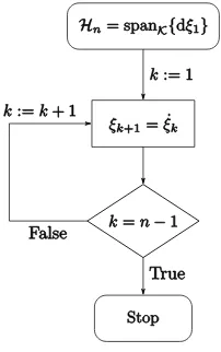
Figure 1 presents the summarized algorithm for computation of the coordinate transformation
( )x
in the case of single-input single-output (SISO) systems.
Figure 1. Computation of coordinate transformation The application of the coordinate transformation
( )x
, obtained using the algorithm from Figure 1, to system (1) yields
1 2
1 ,
, ,
n n
n u
for which it is easy to construct the static state feedback by equating the right-hand side of the last equation to new input .v Note that in the SISO case
1 span d , d1 1
n whereas in the MIMO case to
span n1 one may need an additional vector d .1 In such a case also 1 has to be considered as a state coordinate together with 1, etc. In general, at each step one has to check whether n j is spanned only
3. Symbolic computational tools
Application of advanced theories, in general, requires specific knowledge of certain mathematical technicalities that complicates testing of novel ideas. The algebraic approach, described in Section 2, is of no exception. Technical areas develop so rapidly that information technologies have become the simplest and reliable way to transfer new knowledge into prac-tice. In addition, since solutions of nonlinear control problems require a huge amount of symbolic compu-tations, additional software assistance is of high impo-rtance. Thus, the development of scientific software with a focus on possible practical applications becomes more important. This motivates different research groups to develop specific packages and even stand-alone applications.
Thus, to make a smooth transition of algebraic framework toward practical applications, Computer Algebra System Mathematica-based symbolic package NLControl was created in the Institute of Cybernetics at Tallinn University of Technology [13], [14]. The package encapsulates developed theory providing powerful though simple enough way to tackle a wide range of nonlinear control problems. NLControl has a modular structure and consists of, except assistant functions, the following most important modules depicted in Error! Reference source not found..
Figure 2. Basic structure of NLControl package There are several possibilities to classify the implemented functions, in particular, according to: (i) tasks to be solved, (ii) time domain, (iii) mathematical tools applied, etc. However, the most natural way is to separate functions with respect to modules. The reason is that the main functions are implemented in such a manner that they can solve the same problem for systems defined in different time domains making this way the code more compact, see [15] or visit the project's web page [16].
4. Analysis and control of a Multi-Tank system
The graphical representation of a Multi-Tank sys-tem is presented in Figure 3.From Figure 3 one can see that the overall system consists of three serially connected water reservoirs that have different geometry. The physical meaning of
parameters (omitted in Figure 3) are listed in Table 1, where i1, 2,3 indicates the number of a tank.
Figure 3. Model of the Multi-Tank system
Table 1. Nomenclature
Parameters Physical description
i
x fluid level in the ith tank
w width of a tank
i
C resistance of the output orifice of the ith tank
i
flow coefficient for the ith tank
Some parameters in Table 1 have constant values (units are given in meters): a0.25, b0.345,
0.1,
c R0.364, h0.35, and w0.035. Note that the maximal height of each tank is 0.35m. However, the maximal reachable height may vary with respect to safety requirements and experimental setup. The rest of parameters have to be identified experimentally. In addition, state variables and control signals have natural saturations due to the physical limitations of the system. Note that for the laminar flows the outflow rate from a tank is governed by the Bernoulli's law that corresponds to the case i 1 / 2. In fact, this is a typical assumption made in the academic research. However, in case of real process such issues like turbulence and acceleration of the liquid in the tube cannot be usually neglected. Therefore, in more general cases i(0, 0.5] has to be assumed.
The Multi-Tank system is equipped with valves and level sensors for each tank. The upper tank has a constant cross-sectional area. However, the middle and lower tanks have variable (conic and spheral) cross-sectional areas causing additional nonlinearities in the outflow. The system is equipped with direct current pump providing liquid transportation from the lowest water reservoir to the upper tank. The pump is supplied from the power interface by an appropriate pulse-width modulation control signal. The tank Core
Analysis Modeling
valves can be considered as flow resistors. Each pair (automatic and manual) of valves between tanks can be separately controlled changing this way the output flow and, if necessary, the number of inputs and outputs of the system. Thus, the system can be reconfigured with respect to the pre-specified requirements. Since the system has a flexible configuration, various models can be analyzed on the basis of this prototype. Furthermore, each tank has its own sensor for measuring water level. The plant is designed to operate with an external PC-based digital controller. The computer communicates with the level sensors, automatic valves and pump by a dedicated i/o board and the power interface. The i/o board is controlled by the real-time software which operates in Simulink on the basis of MATLAB Real-Time Windows Target environment.
Due to the flexible structure of the system, numerous different combinations are possible. In what follows, the most important cases are presented. All real-life experiments were performed on the equip-ment available in the laboratory at the Departequip-ment of Computer Control, Tallinn University of Technology, see [17]. For more specific details and assumptions made for the model see the manual available at [18]. 4.1. Pump-controlled scenario
In order to control water level in a tank, we use settings listed in Table 2 for our experiments.
Table 2. Pump-controlled scenario: configuration
Tank # Pump Manual valve Automatic valve
1
varies
fully opened closed
2 fully opened closed
3 fully opened closed
The configuration presented in Table 2 leads to the so-called pump-controlled version of the system in which pump is used as a generator of the control ac-tion (input signal). In this case, differential equaac-tions, describing the dynamics of the system, can be derived, assuming the laminar outflow rate of an ideal fluid from a tank, by means of mass balance as
1
1 2
3 2
1 1 1
2 1 1 2 2
2
3 2 2 2 3 3
2
3
1
1
. x u C x
aw h
x C x C x
cwh bwx
x C x C x
w R R x
(3)
In principle, such configuration allows simultane-ous control of water levels in several tanks. However, this type of control will barely be illustrative. There-fore, in this subsection we restrict our attention to the case of SISO version. Next, we present a detailed analysis of the system and controller synthesis.
Case 1: We start from the water level control in the upper tank, meaning that only the first equation of (3) is used
1
1 1
.
x u C x
aw
(4)
First, we verify the accessibility (controllability) property of the system, since it is a necessary condi-tion for a system to be linearizable. According to (2), the sequence k, k0 can be calculated as follows
0
1
2
span d , d , span d ,
0 .
x u
x
(5)
From (5), we get that : 2 {0}. Therefore, according to Theorem 2, system (4) is accessible. In fact, this conclusion is not surprising, since the chosen configuration is nothing else than the first-order SISO differential equation having input as a separate variable. Obviously, 1 in (5) is completely integrable. Therefore, the conditions of Theorem 2 are satisfied and the system is linearizable via the static state feedback 1
1
uawv C x and no coordinate transformation is necessary. Note that the feedback law is globally defined and does not bring any restric-tions. After applying the static state feedback, we get the following closed-loop system xv. Though this particular combination is relatively simple, we intended to demonstrate the possibilities of algebraic approach. In case of more complex configurations or systems this can significantly simplify analysis and controller synthesis.
Next, the flow coefficient and resistance of the output orifice of the first tank were identified experimentally as
1 0.3488
and 4 2
1 1.6809 10 m /s,
C
respectively, using MATLAB routine provided with the installation package. Note that the input signal is defined as u: 1 2, where
4
1 u t( ) 0 u t( ) 1.2394 10
∣
and
2 u t( ) ∣0u t( ) 1 .
The input signal is scaled to simplify numerical calculations.
of the EKF requires a discrete-time model of the tank system that, in general, can be derived, using Euler sampling method. Further, the EKF is applied to all tanks and used to improve the performance of the control algorithm.
The reference signal v was chosen as a piecewise constant function presented in Table 3.
Table 3. Set points
Value [m] Time interval [s]
0.20 0 t 95 0.05 95 t 180
0.1 180 t 260 0.15 260 t 350
Note that v was chosen intentionally this way to illustrate the ability of the proposed method to per-form in the whole region of set points. The quality of control algorithm is depicted in Figure 4.
Figure 4. Experimental results of the water level control in the first tank. The upper plot shows outputs
(water level). The lower plot reflects the corresponding input signals
Furthermore, the classical PID controller was chosen for comparison purposes. It was obtained using tools available in FOMCON package [19], which encompasses the main tuning functionality providing additional flexibility in terms of fractional-order modeling. The time-domain performance index ITAE (Integral Time Absolute Error) was used during the optimization based tuning procedure resulting in a compensator of the form
1( ) 10 0.28498 / 0.41735 .
Cp s s s
It can be seen from Figure 4 that both control methods are capable of tracking the reference signal v and react correctly to the changes in a set point. Finally, it is important to stress that the same analytic controller works accurately on the whole region of set points unlike the PID controller, which has to be retuned for each working point in order to provide comparable performance quality.
Case 2: Now, we proceed with analysis of the water level control in the second tank, meaning that the first and the second equations of (3) are used
1
1 2
1 1 1
2 1 1 2 2
2
1
. x u C x
aw h
x C x C x
cwh bwx
(6)
In the same manner as in Case 1 we start our analysis from the accessibility property of the system. According to (2), the sequence k, k0 can be calculated as
0 1 2
1 1 2
2 2
3
span d , d , d , span d , d ,
span d , 0 .
x x u
x x
x
Since
0 , the system (6) is accessible.Moreover, the subspace 2 is completely integrable. Therefore, the conditions of Theorem 3 are satisfied.
Now, using Algorithm presented in Section 2, we get the coordinate transformation, given as
1 2
1 22 2 1 1 2 2
2
x
h
x C x C x
cwh bwx
(7)
and the static state feedback as
1
1 1 1 1
1 1
1 1 1
1
1 1 2 1 1
2 1 1
1 1 1
1 2
1 1 2 1 1
1
2 3 1
2 2 1 1
1 1 2
2 2
1 2 1 1 1 2
1 1
1 1 2 2 1 1
1 2
2
2 2 2 2 2 1 1
2 2
( )( )
( ( ) ) ( ( )
( ( ( )
( ) ) ( )
(( 2) ) ( )
(( 1)
(
u aw C H bx cH C Hx
aw x bx cH H C Hx
C x x C H bx cH
abH C Hx aC x C Hx
bx cH aC Hx C Hx bx
2cH)))v
)
.(8)
From (7) and (8) one can find that the proposed control scheme is valid everywhere except when
2 0
x . Note that one can use NLControl website to calculate the corresponding expressions using the function Linearization, which returns the coordinate transformation and the static state feedback. After applying the change of variables (7) and the static state feedback (8), system (6) transforms into the controller canonical form given as
1 2
2
1
, , v y
Next, the flow coefficient and resistance of the output orifice of the second tank were determined experimentally as
2 0.3664
and 4 2
2 1.6184 10 m /s,
C
respectively. The control system was validated using the reference signal v presented in Table 4.
Table 4. Set points
Value [m] Time interval [s]
0.08 0 t 80 0.13 80 t 150 0.09 150 t 250
Experimental results are depicted in Figure 6. In the similar manner as in Case 1 the PID controller was tuned using FOMCON package resulting in
2( ) 47.529 0.35178 / 99.1 .
Cp s s s
One may see that the controller based on analytical approach provides a slightly better performance comp-ared to Cp s2( ) since the latter—the best conventional PID controller obtained for the problem—offers comparable performance qualities in terms of settling time and—to a lesser extent—set-point tracking at the expense of having an underdamped response.
Figure 5. Water level control in the middle tank 4.2. Valve-controlled scenario
It is hard to use only valve-controlled version of the system. This is because one has to predefine the constant power for the pump. The latter is not a simple task, since inappropriate value will result in poor control results (for example, too small value yields lack of water). However, there exists a configuration interesting from the analysis point of view. Note that in case of valve-controlled system differential equations are very similar to (3) except that u becomes a fixed constant q:u t( )
0,1 and,
i
C for i1, 2,3, can be used as control inputs instead. Consider settings (note that v:C3 is an input of the system) listed in Table 5.
Table 5. Valve-controlled scenario: configuration
Tank # Pump Manual valve Automatic valve
1
constant
fully opened closed
2 fully opened closed
3 closed varies
Configuration presented in Table 5 yields
1
1 2
3 2
1 1 1
2 1 1 2 2
2
3 2 2 3
2 2
3
1
1
. x q C x
aw h
x C x C x
cwh bwx
x C x vx
w R R x
(9)
The sequence k can be calculated as
0 1 2 3
1 1 2 3
2 1 2
3 1 2
span d , d , d , d , span d , d , d ,
d , d , d , d : .
x x x u
x x x
x x
x x
Though configuration presented in Table 5 at the first sight seems to be reasonable, according to Theorem 3, the system is not accessible. From 3 one can easily find the dynamics of autonomous subsystem, described by first two equations of (9), yielding that there is no possibility to influence x1 and
2
x via input signal, and the water in the lower tank is the only state that can be controlled. Though the same conclusion can be obtained from the physical meanings and description of the plant, the algebraic approach provides a compact way to understand the various properties of a system, in this particular case, accessibility.
4.3. Pump/valve-controlled scenario
Here, we want to cover the case of simultaneous control of water level in several tanks using pump and automatic valves. Consider settings listed in Table 6.
Table 6. Pump/valve-controlled scenario: configuration
Tank # Pump Manual valve Automatic valve
1
varies
fully opened varies
2 fully opened closed
3 fully opened closed
1 1
1 1 2
1 1 2 1 1 1
2 2 1 1 1 2 2
2
1
. x u u x C x
aw h
x u x C x C x
cwh bwx
(10)
The sequence k, k0 can be calculated as
0 1 2 1 2
1 1 2
2
span d , d , d , d , span d , d ,
0 : ,
x x u u
x x
yielding that system (10) is accessible. Moreover, the subspace 1 is completely integrable. Therefore, the conditions of Theorem 3 are satisfied. Observe that there is no need for coordinate transformation. Thus, we equate the right-hand sides of (10) to v1 and v2, respectively, and solve the corresponding equations with respect to u1 and u2, yielding the static state feedback given as
2
2 1
1
2
1 1 2 2 2
2 2 2 1 1 2 2
1 1
. bx
u awv C x wv c
h
u hC x hC x wv ch bx
hx
(11)
Note that control law (11) is valid in the region where x10 . Application of the feedback (11) transforms the state equations (10) into the form
1 1, 2 2.
x v x v The parameters 1, 2 and C C1, 2 were already identified in the previous experiments. Outputs are chosen to be water levels in the first and second tanks, respectively, i.e., y1x1 and y2 x2. Changes of set points are presented in Table 7.
Table 7. Reference signals changes
1
v [m] v2 [m] Time instance [s]
0.05 0.1 0
0.05 0.15 95
0.07 0.15 130
The experimental results are depicted in Figure 6. It can be seen that the outputs of the system are capable of tracking the reference signals.
5. Conclusions
In this paper, the algebraic framework, based on the theory of differential one-forms, has been applied to analyze the Multi-Tank system [17]. This frame-work allows one to study typical system properties, in particular, accessibility and feedback linearizability using the same mathematical tools. The intention was to illustrate the potential applicability of the frame-work to the real-life problems. The water tank system was used as an example due to several reasons. In par-ticular, this is a prototype of processes widely
occur-ring in chemical and food processing industry. More-over, the system is used in various educational courses in different universities to illustrate the main theore-tical and practheore-tical concepts of control theory.
Figure 6. The upper plot represents experimental results of water levels in the first and second tanks.
The lower plot depicts the corresponding control signals
Acknowledgments
We would like to present our thanks to anonymous reviewers for their helpful suggestions. Ü. Kotta was supported by the Estonian Research Council, personal research funding grant PUT481.
References
[1] K. J. Åström, T. Hägglund. The future of PID control. Control Engineering Practice, 2001, Vol. 9, No. 11, 1163–1175.
[2] G. Conte, C. H. Moog, A. M. Perdon. Algebraic Methods for Nonlinear Control Systems. Springer-Verlag, London, 2007.
[3] Ü. Kotta, P. Kotta, M. Halás. Reduction and transfer equivalence of nonlinear control systems: unification and extension via pseudo-linear algebra. Kybernetika, 2010, Vol. 46, No. 5, 831–849.
[4] J. Belikov, Ü. Kotta, M. Tõnso. Adjoint polynomial formulas for nonlinear state-space realization. IEEE Transactions on Automatic Control, 2014, Vol. 59, No. 1, 256–261.
[5] K. H. Johansson. The quadruple-tank process: A multivariable laboratory process with an adjustable zero. IEEE Transactions on Control Systems Techno-logy, 2000, Vol. 8, No. 3, 456–465.
[6] W. C. Dunn. Fundamentals of Industrial Instrumenta-tion and Process Control. McGraw-Hill Professional, 2005.
[7] C. Kern, M. Manness. PID controller tuning for mixed continuous/discrete event processes using dyna-mic simulation. In: Proceedings of Dynamic Modeling Control Applications for Industry Workshop, Vancou-ver, BC, Canada, 1997, pp. 37–43.
[8] A. Tepljakov, E. Petlenkov, J. Belikov, M. Halás.
the 32nd American Control Conference, Washington, DC, USA, 2013, pp. 1780–1785.
[9] E. Kolchin. Differential Algebra and Algebraic Groups. Academic Press, London, 1973.
[10] Y. Choquet-Bruhat, C. DeWitt-Morette, M. Dilla-rd-Bleick. Analysis, Manifolds and Physics, Part I: Basics. North-Holland, Amsterdam, The Netherlands, 2004.
[11] L. C. To, M. O. Tadé, M. Kraetzl. Robust Nonlinear Control of Industrial Evaporation Systems: Implemen-tation of Differential Geometric Techniques. World Scientific, Singapore, 1999.
[12] T. Mullari, Ü. Kotta, M. Tõnso. Static state feedback linearizability: relationship between two methods. Proceedings of the Estonian Academy of Sciences, 2011, Vol. 60, No. 2, 121–135.
[13] J. Belikov, Ü. Kotta, M. Tõnso. Symbolic polynomial tools for nonlinear control systems. In: Proceedings of the 7th Vienna International Conference on Mathema-tical Modelling, Vienna, Austria, 2012, pp. 1–6.
[14] J. Belikov, Ü. Kotta, M. Tõnso. NLControl: Symbolic package for study of nonlinear control systems. In: Proceedings of the Multi-Conference on Systems and Control, Hyderabad, India, 2013, pp. 322–327. [15] M. Tõnso, H. Rennik, Ü. Kotta. WebMathematica
based tools for discrete-time nonlinear control systems. Proceedings of the Estonian Academy of Sciences, 2009, Vol. 58, No. 4, 224–240.
[16] Institute of Cybernetics at Tallinn University of Technology. (2015). NLControl website, [Online]. Available: http://www.nlcontrol.ioc.ee.
[17] ALab. (2015). Alpha Control Laboratory, Tallinn University of Technology, [Online]. Available:
http://a-lab.ee/.
[18] INTECO Sp. z o. o. (2013). INTECO, [Online]. Available: http://www.inteco.com.pl.
[19] A. Tepljakov, E. Petlenkov, J. Belikov. FOMCON: A MATLAB toolbox for fractional-order system identifi-cation and control. International Journal of Microelec-tronics and Computer Science, 2011, Vol. 2, No. 2, 51–62.