A Two-Stage Taguchi Design Example-image Quality Promotioin Miniature Camera/Cell-Phone Lens

A Two-Stage Taguchi Design Example



Image Quality Promotion in

Miniature Camera/Cell-Phone Lens

Luke K. Wang

, Jen-Yu Shieh

, Kun-Hsien Lin

and Ken Huang

1

Department of Electrical Engineering, National Kaohsiung University of Applied Sciences, Kaohsiung, Taiwan

2

Department of Electro-optics Engineering, National Formosa University, Hue-Wei, Yue-Ling County 632, Taiwan

3

Arc Precision Technology Co., Ltd., Taichung, Taiwan

Received 11 April 2012; received in revised form 15 May 2012; accepted 20 June 2012

Abstract

A simple, practical manufacturing process, integrating manufacturing capability-oriented design (MCOD)

philosophy and Taguchi’s method, is presented to tackle the high resolution miniature camera/cell phone lens

issues at the manufacturing phase. Meanwhile, we also use optical software to create an analytical simulation model

to investigate the quality characteristics due to lens’ thickness, eccentricity, surface profile, and air lens’ gap; a single

quality characteristics expressed in terms of modulation transfer function (MTF) is defined. Optimal combination of

process parameters in experimental scenario using Taguchi’s method is performed, and the results are judged and

analyzed by the indices of signal-to-noise ratio (S/N) and the analysis of variance (ANOVA). The key idea of the

two-stage design is to utilize optical software to conduct the sensitivity analysis of MTF first; an analytical model,

dependent on actual process parameters at manufacturing stage, is constructed next; and finally by substituting these

outputs from the analytical model back to the optical software to verify the design criterion and do the modifications.

By minimizing both the theoretical errors at design stage and the complexity in the manufacturing process, we are

able to seeking for the most economical solution, simultaneously attain the optimal/suboptimal combination of

process parameters or control factors in lens manufacturing issue.

Keywords: Taguchi Method, MTF, Lens

1.

Introduction

Taguchi method [1-2] basically focuses on the design of experiments, determining the couplings between the quality

characteristics (output) and the control factors (input), possessing a certain number of levels. Taguchi method has been

popular in the fields of optical and lens designs/manufacturing. Use of both Taguchi method and principle component analysis

(PCA) to achieve multiple performance characteristics (MPC) (or multi-objective) for a U-type 2X zoom projection lens set

was presented in section 3. The system complexity was increasing, and the SPSS software was employed to generate the

outputs with the corresponding given inputs, i.e., the training procedure is unavoidable and necessary for obtaining principle

components. By combining fuzzy-logic with Taguchi method, a successful simulation was claimed, that is, eliminating

primary aberrations for U-type 2X zoom optics with freeform surface.[3-4]

*Corresponding author. E-mail address: [email protected]

A new concept for the optimization and optical design[5] of miniature digital zoom optics with liquid lens elements is

proposed in this research. It propose a newly developed digital zoom layout and optimization with a modified genetic algorism

(GA) method, in order to meet the demands of a certain specification. The results show that achieve a successful optical design

and the optimization of the digital zoom optics with liquid optics, whose performance is greatly improved up to 48.68%, from

the standpoint of onaxis spot size.From the photographer point of view, contrast and resolution are nevertheless in conflict.

One fair index for the quality analysis in photorgraphy is the modulation trasfer function (MTF), describing the complex

interaction between resolution and contrast. Eventually, MTF is adopted to be the quality characteristics here.

The ultimate goal of our design is to design an simple, alternative manufacturing process for lens manufacturing to

accelerate the time-to-market instead of using the aforementioned methods with high system complexity in software, hardware,

or manufacturing processes. In this analysis, an orthogonal array, consisting of a number of 18 experiments, 8 control factors

with each maintaining 3 levels except the first one, which is only containing 2 levels, is constructed to enhance the quality

characteristics, MTF, in our case. Interaction issue is hereafter not discussed and neglected herein.

2.

Design methodology

In Taguchi’s method, the quality characteristics are usually divided into (1) nominal-is-best, (2) smaller-the-better, and

(3) larger-the-better. The flow chart of a design of experiment for our case is shown in Fig. 1.

The magnitude of the optical transfer function (OTF), describing the spatial variation as a function of spatial frequency,

is known as the modulation transfer function (MTF). MTF may be used to evaluate the imaging quality as well as the contrast

issue in photography. The spatial frequency is expressed in lp/mm( line pairs per mm). Optical analysis stage is to determine

the degree of reliance of the MTF; we make use of the optical software to determine the degree of coupling of MTF with some

of the system/process parameters (control factors). At the stage of the construction of a simulation model, process parameters

of the manufacturing system come into the view. Therefore, the set of control factors can be selected, and the number of levels

for each control factor can be determined accordingly. The orthogonal array can be established. After the employment of

software simulation, analysis through both signal-noise-ratio (S/N) and analysis of variance (ANOVA) is applicable. Optimal

parametric combination of control factors with associated levels can be done by those dominant factors and levels summarized

in the S/N and ANOVA tabulations.

Fig. 1 The block diagram for the proposed scenario

Generally speaking, the performance of the quality characteristics can be evaluated through the three indices, defined by

Taguchi, namely, the smaller-the-better (SB), the nominal-the-best (NB), and the larger-the-better (LB), all expressed in db;

} 1 log{ 10

1 2



 n

i i

SB y

n

} 1 1 log{ 10

1 2



 

 n

i i

NB

y n



} log{

10 ₂

S y

LB 

 (3)

where

yi: quality characteristics

y: expectation of y

S2: sample variance.

3.

Experiment

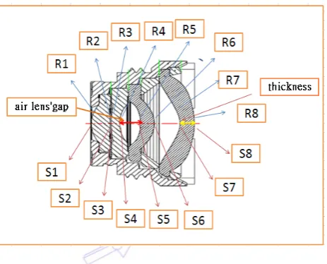
A prototype lens assembly with four aspherical lens mounted in a cascade manner is introduced for the experiment.[6-8]

Assignments of lens’ parameters are shown in Fig. 2, where R stands for radius while S means surface. Owing to the

requirements of light weight and miniature size for optical lens, plastic material is employed.

Fig. 2 The assignments of lens’ numbers

Speaking of the MTF values selected for this paper, spherical aberration, coma and astigmatic will affect the sharpness

of the image field curvature. Distortion will only result in a change of image position and shape had no effect on the resolution,

which is incorrect aberration. Distortion and field curvature repair very good but let MTF values can not meet the requirements,

because the aberration is not likely to be fully eliminated.

3.1. Sensitivity Analysis

We propose the use of optical software to accomplish the sensitivity analysis of lens manufacturing. Arbitrarily

choosing MTF equal to 80 lp/mm along tangential direction (sampling at 0.5F, 0.7F, and 0.9F) and setting object location at

infinity, we can easily visualize which control factor should be included in the degree of reliance (DOR) or sensitivity analysis.

The results are tabulated in Table 1. Those highlighted grids are so significant for the sensitivity analysis, and are therefore

recruited for analysis. For example, if the misplaced quantity is 0.003mm for L1R1 (radius of lens #1), the degradation of

Table 1 Sensitivity analysis of MTF

Ranking Description Tolerance

_MTF

0. 5F 0. 7F 0. 9F 6 8% 6 0% 5 5%

1 L1R1 misplaced 0.003mm 0% 0% -1%

0.003mm -13% -20% -23%

2 L1R1 tilt &

misplaced

0.003mm 0% 0% 0%

0.003mm -11% -17% -17%

3 L2R2 misplaced 0.003mm -10% -15% -16%

0.003mm 0% 0% 0%

4 L2R1 misplaced 0.003mm 0% 0% 0%

0.003mm -14% -15% -8%

5 L3R1 misplaced 0.003mm 0% 0% -6%

0.003mm 0% 0% 0%

6 L1 thickness 0.005mm -1% -1% 2%

0.005mm 1% 0% -2%

6 L1L2 air lens’ gap 0.005mm -1% -2% -2%

0.005mm -1% 1% 1%

6 L2L3 air lens’ gap 0.005mm -1% 1% 2%

0.005mm 1% -1% -2%

7 L2 thickness 0.005mm 0% 0% 1%

0.005mm 0% 0% -1%

7 L3 thickness 0.005mm 0% 0% 1%

0.005mm 0% 0% -1%

7 L3L4 air lens’ gap 0.005mm 0% 1% 1%

0.005mm 0% -1% -1%

3.2. Analytical Model

Table 2 The feasible process parameters in manufacturing system

L1 specification measured L2 specification Measured

Outer diameter 2.90.005 2.911 Outer diameter 3.50.005 3.511

thickness 0.750.005 0.753 thickness 0.330.005 0.336

Air lens’ gap (L1-L2)

0.050.005 0.061 Air lens’gap

(L2-L3)

0.830.005 0.8205

S1 absolute 00.003 0.00545 S3 absolute 00.003 0.01028

S2 absolute 00.003 0.00528 S4 absolute 0+0.003 0.00227

Total 00.003 0.00143 Total 00.003 0.01219

Best R1 -X N/A 1.6003 Best R3 -X N/A 9.9967

Best R1-Y N/A 1.6 Best R3 -Y N/A 10.035

Best R2-X N/A 7.475 Best R4 -X N/A 1.90401

Best R2-Y N/A 7.45 Best R4 -Y N/A 1.904802

L3 Specification Measured L4 specification Measured

Outer diameter 3.90.005 3.904 Outer diameter 5.40.005 5.397

thickness 0.550.003 0.552 thickness 0.570.005 0.571

Air lens’gap (L3-L4)

1.0210.005 1.0205 Air lens’gap (L4- )

N/A N/A

S5 absolute 00.003 0.0024 S7 absolute 00.003 0.0078

S6 absolute 00.003 0.0093 S8 absolute 00.003 0.0015

Total 00.003 0.0080 Total 00.003 0.0093

Best R5 -X N/A 2.5430 Best R7 -X N/A 1.2500

Best R5 -Y N/A 2.5430 Best R7 -Y N/A 1.2493

Best R6 -X N/A 1.4995 Best R8-X N/A 3.4910

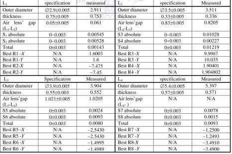
Experiment is performed after the sensitivity analysis with the help via optical software. Uncontrollable and unexpected

consequences associated with selected factors may come to the view when the output dataset from optical software analysis is

directed to the manufacturing phase. In order to simulate the lens’ manufacturing process as close as possible to the actual

scenario, we establish a process parameters-directed, analytical simulation model. By referring to the actual experimental

results, those factors having substantial degree of significance related to the MTF are back substituted to the optical software to

improve the quality characteristics. The manufacturing capability is characterized through the numeric summarized in Table 2

with all units in mm. The factors associated with the process parameters to be used in the manufacturing stage are thickness

(L1 to L4), eccentricity (lateral offset and tilt), surface profile (best R value), and the air lens’ gaps.

3.3. Orthogonal Array Selection

The relationship between lens’ optical parameters and actual manufacture tolerance for each lens’ component is

investigated. Our design philosophy is to wisely pick up those control factors/parameters. A variety of test-beds is making our

experiment scenario complicated.[9-11] For simplicity, the default values for the experiment issue are  finite location to

infinity for object, spatial frequency set to120 lp/mm, and the outputs are MTF values along tangential direction. The MTF test

point locations are illustrated in Fig. 3. Those three concentric circles are the locations for 50%, 70%, and 100% of image

heights.

Fig. 3 Illustration of MTF sampling locations

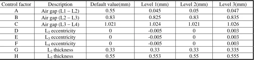
There are eight control factors in our experiment, and the number of experiments to be conducted is 6561 with three

levels for each control factor. Alternatively, a L18 orthogonal array is adopted to reduce the number of experiments down to

18, provided that one of these control factor’s levels needs to be adjusted to 2. We arbitrarily choose the first control factor, the

air gap between lens #1 and lens #2. A complete list of control factors and their associated levels is in Table 3, and the L18

orthogonal array is referred to Table 4. Noticed that the level 3 of control factor “A” is intentionally neglected due to the use

of L18 array instead of L27(313) array.

Table 3 List of the control factors and associated levels

Control factor Description Default value(mm) Level 1(mm) Level 2(mm) Level 3(mm)

A Air gap (L1  L2) 0.55 0.045 0.05 0.047

B Air gap (L2  L3) 0.83 0.825 0.83 0.835

C Air gap (L3  L4) 1.021 1.024 1.021 1.026

D L2 eccentricity 0 -0.005 0 0.003

E L3 eccentricity 0 -0.005 0 0.003

F L4 eccentricity 0 -0.005 0 0.003

G L2 thickness 0.33 0.33 0.33 0.335

Table 4 Simulation using L18 orthogonal array and its corresponding MTF and signal-to-noise ratios

After substituting the listed parameters shown in Table 3 and Table 4 and the entries in the orthogonal array L18(2137)

into optical software, the corresponding MTF values and their computed S/N ratios are listed in Table 4. The quality

characteristics chosen is the MTF, and the selected S/N ratio is the larger-the-better. It is expressed as

(S/N)larger-the-better = 



 n

i

i

n 1

) 2 MTF

1 1 log(

10 (4)

where n is the number of experiments being conducted. The impact of S/N versus control factors with designated levels

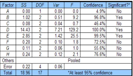
is drawn in Fig.4. The impact of quality characteristics, MTF, versus control factors is shown in Fig.5. ANOVA is therefore

performed to confirm the significances of those selected control factors, based on the setting of 95% confidence interval; the

results are illustrated in Table 5. The degree of significance is marked by either “yes” or “no.”

The degree of contribution of variance can be visualized via the column termed “F,” the F-ratio test. The ranking is as

follow  D, E, and B. The contribution of the optical system up to the greatest impact, which control factor D, confidence of

the highest 100% probability that can enhance the quality characteristics, followed by control factor E, respectively, 99.5%

probability, 96.8% probability.

Fig. 4 The impact of S/N versus control factors

Fig. 5 The impact of quality characteristics, MTF, versus control factors

3.4. Optimal Parameters Combination

In summary, we perform the optical analysis via software, the impacts of MTF with various control factors with levels,

and finally the ANOVA. The optimal combination/selection of control parameters becomes obvious. Initially, the decision is

made, and the optimal parameter set is {B3, D2, E1}. The degree-of-reliance (DOR) to the quality characteristics is further

categorized into three classes. The optimal parametric combination is therefore sought. For the purpose of analysis, Table 6

shows the classification of the control factors. In Table 6, Q.C. stands for quality characteristics. By adjusting the factors in

class #1 to maximize the S/N, we obtain the following combination, A*-B3-C*-D2-E1-F*-G*-H*, where ()* stands for that

user can select any of the corresponding levels (1-3); those factors belonging to class #2 are tuned next. Finally, the ultimate

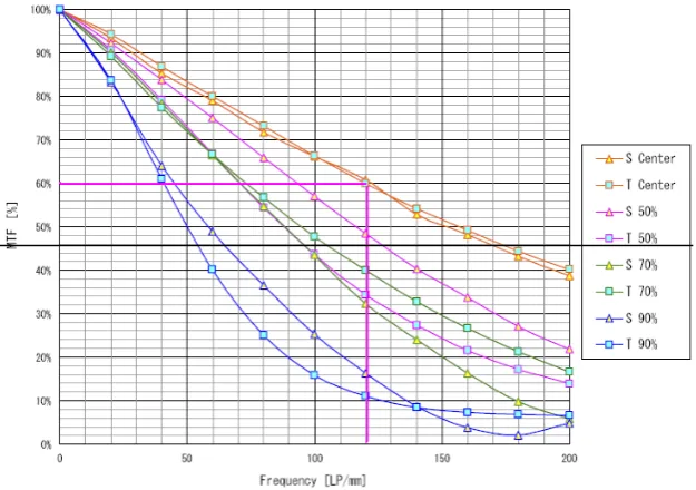
optimal combination is A1(orA2)-B3-C3-D2-E1-F3-G1-H3. The response curves of MTF before and after the introduction of

Taguchi design are plotted in Fig.7 and Fig.8, illustrating the increasing of MTF values from 55.6% to 60% at the spatial

frequency of 120 lp/mm. The preceding analysis and the choosing of optimal control factors with assigned level are directed to

the lens manufacturing. The manufactured high-resolution camera/cell-phone lenses are included in Fig.6. Multiple

performance characteristics (MPC) may be recruited to have further improvement in lens manufacturing issue, but the design

complexity and the computational load will be increased tremendously.The improvement of S/N comparing to the original

default/design specs, choosing {B3, D2, E1}, is

 (S/N) = 0.02 + 0.06 = 0.08. (5

) where ( ) stands for difference operation. Actually, the increment of S/N value confirms the effort in seeking the

optimal combination of control factors.

Table 6 Classification of control factors

class Coupled with S/N Coupled with Q.C. Control Factor Purpose

1 Yes Yes/No B,D,E Variation minimization

2 No Yes C,F,G,H Desired Q.C.

Fig. 6 The manufactured high-resolution camera/cell-phone lenses using the Taguchi design

Fig. 7 The impact of MTF vs. frequency before the introduction of Taguchi method (S:Sagital, T:Tangential)

4.

Conclusions

An effort to promote the image quality via the increasing of the value of modulation transfer function throughout the

generic two-stage design has been proposed and verified through software simulation with two key features, signal-to-noise

ratio and the analysis of variance, and may finally be directed to mass production process. With the help from the analysis

using optical software, a simulation model is constructed and incorporated with Taguchi’s method to fulfill the ultimate goal,

i.e., cost reduction and shortening developmental or enter-to-market time; meanwhile, the optimal/suboptimal combination of

the process parameters is obtained. Those most significant control factors relating to the quality characteristics, MTF, are

analyzed. The comparisons of responses (MTF) between the manufactured and the designed are conducted. Those crucial

control factors chosen are very common in lens manufacturing industries. Instead of employing trial-and-error strategy to

promote the quality of high resolution lens, the proposed analysis combing Taguchi method with analysis of variance is, for

sure, simple, practical, and applicable in a variety of applications. It also provides a guideline to the manufacturing of miniature

lens, exclusively with the manufacturing capability-oriented design criteria in a manufacturing process.

References

[1] Walia, R. S., H. S. Shan and P. Kumar, “Multi-response optimization of CFAAFM process through Taguchi method and utility concept. Materials and Manufacturing Processes,” vol. 21, pp. 907-914, 2006.

[2] Wikipedia, “Taguchi methods,” http://en.wikipedia.org/wiki/Taguchi_methods.

[3] N. Jin and Y. Rahmat-Samii, “A novel design methodology for aperiodic arrays using particle swarm optimization,” in 2006 Nat. Radio Sci. Meeting Dig., Boulder, CO, Jan. 2006, pp. 69–69.

[4] A. S. Hedayat, N. J. A. Sloane, and J. Stufken, Orthogonal Arrays: Theory and Applications. New York: Springer-Verlag, 1999.

[5] Yi Chin Fang, Tung-Kuan Liu, Cheng-Mu Tsai, Jyh-Horng Chou, Han-Ching Lin and Wei Teng Lin “Extended optimization ofchromatic aberrations via a hybrid Taguchi–genetic algorithm for zoom optics with a diffractive optical element,” J. Opt. A: Pure Appl. Opt. vol. 11, Apr. 2009.

[6] C. R. Rao, “Factorial experiments derivable from combinatorial arrangements of arrays,” J. Roy. Statist. Soc., vol. 9, pp. 128–139, 1947.

[7] Dongcheol Kim and Sehun Rhee, Ieee Trans. On System, Man, and Cybernetics, Part B, vol. 32, pp.157-162, Apr. 2002. [8] I.S. Kim, K.J. Son, Y.S. Yang, P.K.D.V. Yaragada, Int. J. Machine Tools & Manufacture, vol. 43, pp.763-769, June 2003. [9] Michael P. L., “Arbitrarily profiled 3D polymer MEMS through Si micro-moulding and bulk

micromachining,” Microelectronics Engineering, vol. 83, pp.1257-60, 2006.

[10]Su, C. T., Chiu, C. C. and Chang, H. H., “Parameter design optimization via neural network and genetic algorithm,” International Journal of Industrial Engineering, vol. 7, pp. 224-231, 2000.