Dynamic Hierarchical Markov Random Fields for Integrated Web
Data Extraction
Jun Zhu [email protected]
Department of Computer Science and Technology Tsinghua University
Beijing, 100084, China
Zaiqing Nie [email protected]
Web Search and Mining Group Microsoft Research Asia Beijing, 100080, China
Bo Zhang [email protected]
Department of Computer Science and Technology Tsinghua University
Beijing, 100084, China
Ji-Rong Wen [email protected]
Web Search and Mining Group Microsoft Research Asia Beijing, 100080, China
Editor: John Lafferty
Abstract
Existing template-independent web data extraction approaches adopt highly ineffective decoupled strategies—attempting to do data record detection and attribute labeling in two separate phases. In this paper, we propose an integrated web data extraction paradigm with hierarchical models. The proposed model is called Dynamic Hierarchical Markov Random Fields (DHMRFs). DHMRFs take structural uncertainty into consideration and define a joint distribution of both model structure and class labels. The joint distribution is an exponential family distribution. As a conditional model, DHMRFs relax the independence assumption as made in directed models. Since exact inference is intractable, a variational method is developed to learn the model’s parameters and to find the MAP model structure and label assignments. We apply DHMRFs to a real-world web data extraction task. Experimental results show that: (1) integrated web data extraction models can achieve significant improvements on both record detection and attribute labeling compared to decoupled models; (2) in diverse web data extraction DHMRFs can potentially address the blocky artifact issue which is suffered by fixed-structured hierarchical models.
Keywords: conditional random fields, dynamic hierarchical Markov random fields, integrated
web data extraction, statistical hierarchical modeling, blocky artifact issue
1. Introduction
Rexa (http://rexa.info). Recent work has shown that template-independent approaches to extracting meta-data for the same type of real-world objects are feasible and promising. However, existing approaches use highly ineffective decoupled strategies—attempting to do data record detection and attribute labeling in two separate phases. This paper is to first propose an integrated web data ex-traction paradigm with hierarchical Markov Random Fields, and then address the blocky artifact issue (Irving et al., 1997) with Dynamic Hierarchical Markov Random Fields.
A Motivating Example: we begin by illustrating the problem with an example, drawn from an actual application of product information extraction under our Windows Live Product Search project (http://products.live.com). The goal is to extract meta-data about real-world products from every product page on the Web. Specifically, for crawled webpages, we first use a classifier to select product pages and then extract the Name, Image, Price, and Description of each product from the identified product pages. Our statistical study on 51K randomly crawled webpages shows that about 12.6 percent are product pages. That is, there are about 1 billion product pages within a search index containing 9 billion crawled webpages. If only half of them are correctly extracted, we will have a huge collection of meta-data about real-world products that could be used for further knowledge discovery and data management tasks, such as comparison shopping and user intention detection.
However, how to extract product information from webpages generated by many (maybe tens of thousands of) different templates is non-trivial. One possible solution is that we first distinguish webpages generated by different templates, and then build an extractor for each template; this type of solution is template-dependent. Template-dependent methods are impractical for two reasons. First, accurately identifying webpages for each template is a far from trivial task because even webpages from the same website may be generated by dozens of templates. Second, even if we can distinguish webpages, the learning and maintenance of so many different extractors for different templates will require substantial efforts.
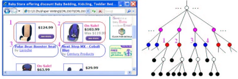
Fortunately, recent work (Lerman et al., 2004; Zhai and Liu, 2005; Zhu et al., 2005) has shown the feasibility and promise of template-independent meta-data extraction for the same type of ob-jects. We can simply combine the existing techniques to build a template-independent extractor for product pages. Specifically, two types of webpages—list pages and detail pages1—are needed to be treated by existing extraction methods. List pages are webpages containing several structured data records, and detail pages are webpages only containing detailed information about a single object. Figure 1 illustrates these two types of pages. For list pages, we can first use the methods by Zhai and Liu (2005) Lerman et al. (2004) to detect data records and then use the model by Zhu et al. (2005) to label the data elements within the detected records. Similarly, for detail pages we can first use the methods by Song et al. (2004) to identify a main data block of a detail page, and then use the same model from Zhu et al. (2005) to do attribute labeling for the elements in the main block.
However, it is highly ineffective to use decoupled strategies—attempting to do data record de-tection and attribute labeling in two separate phases. The reasons for this are:
Error Propagation: as record detection and attribute labeling are two separate phases, the errors in record detection will be propagated to attribute labeling. Thus, the overall performance is limited and upper-bounded by that of record detection.
Lack of Semantics in Record Detection: human readers always take into account semantics of the text to understand webpages. For instance, in Figure 1(a), when claiming a block is a data record, we use the evidence that it contains a product’s name, image, price, and description. Thus,
(a) A list page with two data records. The first record contains 7 elements and the second contains 8 elements.
(b) A detail page contains one product item.
Figure 1: A sample list page and a detail page.
more effective record detection algorithms should take into account the semantic labels of the text, but existing methods (Zhai and Liu, 2005; Lerman et al., 2004) do not consider them.
First-Order Markov Assumption: for webpages, especially detail pages, long-distance depen-dencies always exist between different attribute elements. This is because there are always many irrelevant elements or noise elements appearing between the attributes. For example, in Figure 1(b) there are several noise elements, such as “Add to Cart” and “Select Quantity”, appearing between the price and description. However, plat models like 2D CRFs (Zhu et al., 2005) cannot incorporate long-distance dependencies because of their first-order Markov assumption.
To address the above problems, the first part of this paper is to propose an integrated web data extraction paradigm. Specifically, we take a vision-tree representation of webpages and define both record detection and attribute labeling as assigning semantic labels to the nodes on the trees. Then, we can define the integrated web data extraction that performs record detection and attribute labeling simultaneously. Based on the tree representation, we define a simple integrated web data extraction model—Hierarchical Conditional Random Fields (HCRFs), whose structures are determined by vision-trees.
However, for HCRFs, their structures may not be the most appropriate for web data extraction. This is because when constructing the vision-tree of each webpage, it is unaware of semantic labels. Thus, they cannot resolve all ambiguities. This will lead to those cases in which some closely related nodes may be separated significantly and only connected through a remote ancestor node on the tree. Due to the model’s local Markov assumption, it will lose some useful dependencies and result in low accuracy. An extreme case is that the attributes of different objects are intertwined. Figure 2 shows an example where the two neighboring records on the webpage have their attributes intertwined on the corresponding tree. In this case, fixed-structured hierarchical models are incapable of re-organizing them correctly. This problem has been generally known as blocky artifact issue in image processing (Irving et al., 1997).
Figure 2: An intertwined example webpage. Blocks 1 and 3 present information of one product and blocks 2 and 4 present information of another product. But on the right tree, the information is not correctly grouped.
In undirected dynamic models, parameter estimation is generally intractable, especially when there are hidden variables—both structures and inner variables are hidden in our study. We develop a variational algorithm within the paradigm of contrastive divergence mean field learning (Welling and Hinton, 2001) to do parameter estimation and to find the MAP assignment of labels and the most likely model structures. The performance of our models is demonstrated on a web data extraction task—production information extraction. The results show that: (1) integrated web data extraction models can significantly improve the performance of both record detection and attribute labeling compared to decoupled methods; (2) Dynamic Hierarchical Markov Random Fields can (partially) avoid the blocky artifact issue and achieve high extraction accuracy without tedious manual label-ing of inner nodes, which is required in the learnlabel-ing of the fixed-structured models; (3) integrated extraction models can generalize well to unseen templates. Note that the model is general and could be applied to other fields. We leave further examinations as future work.
The rest of the paper is organized as follows. In the next section, we discuss some background knowledge on which this work is based. Section 3 presents an integrated web data extraction paradigm and fixed-structured Hierarchical Conditional Random Fields. Section 4 describes Dy-namic Hierarchical Markov Random Fields, including an approximate inference algorithm. Section 5 describes implementation details and experimental setup on the task of product information ex-traction. Section 6 and 7 presents evaluation results. Section 8 brings this paper to a conclusion and some future research directions are discussed. Finally, we give our acknowledgements.
2. Preliminary Background Knowledge
The background knowledge, on which the following work is based, is from web data extraction and statistical hierarchical modeling. We introduce these two fields in turn.
2.1 Web Data Extraction
structural dependencies between HTML elements exist. For example, the HTML tag tree is itself hierarchical and each webpage is displayed as a two-dimensional image to readers. Leveraging the two-dimensional spatial information to extract web data has been studied (Zhu et al., 2005; Gatterbauer et al., 2007). This paper is to explore both hierarchical and two-dimensional spatial information for more effective web data extraction.
Wrapper learning approaches (Muslea et al., 2001; Kushmerick, 2000) are template-dependent. They take in some manually labeled webpages and learn some extraction rules (or wrappers). Since the learned wrappers can only be used to extract data from similar pages, maintaining the wrappers as web sites change will require substantial efforts. Furthermore, in wrapper learning users must provide explicit information about each template. So it will be expensive to train a system that ex-tracts data from many web sites. The methods by Embley et al. (1999), Buttler et al. (2001), Chang and Lui (2001), Crescenzi et al. (2001) and Arasu and Garcia-Molina (2003) are also template-dependent, but they do not need labeled training data. They produce wrappers from a collection of similar webpages.
The methods by Zhai and Liu (2005), Lerman et al. (2004) and Gatterbauer et al. (2007) are template-independent. In work by Lerman et al. (2004), data on list pages are segmented using the information from their detail pages. The need of detail pages is a limitation because automatically identifying links that point to detail pages is non-trivial and there are also many pages that do not have detail pages behind them. Zhai and Liu (2005) proposed to detect data records using string matching and also some visual features to achieve better performance, but no semantics are consid-ered. Like the work by Zhu et al. (2005), a general 2D visual model was proposed by Gatterbauer et al. (2007) to extract web tables. The data extracted by the methods of Zhai and Liu (2005), Ler-man et al. (2004) and Gatterbauer et al. (2007) have no seLer-mantic labels. Our work (Zhu et al., 2005) is complementary to this and assigns semantic labels to the extracted data.
2.2 Statistical Hierarchical Modeling
Multi-scale or hierarchical statistical modeling has shown great promise in image labeling (Kato et al., 1993; Li et al., 2000; He et al., 2004; Kumar and Hebert, 2005) and human activity recognition (Liao et al., 2005). Based on whether data are observed at multiple scales, two scenarios exist in which hierarchical modeling is appropriate. First, data are observed at different spatial scales and a model is used to integrate information from the different scales. Second, data are observed only at the finest scale and a model is used to induce a particular process at that scale. The introduced intermediate processes or variables can incorporate more complex dependencies to help the target labeling. Another merit of hierarchical models is that they admit more efficient inference algorithms compared to flat models (Willsky, 2002).
intu-ition, Dynamic Trees (Williams and Adams, 1999) have been proposed, which also consist of two parts—model of structures and model of class labels. However, the difference between DHMRFs and Dynamic Trees is that DHMRFs are defined as exponential family distributions and thus admit several advantages as discussed in the introduction.
Incorporating evidence at various scales was examined in a generative manner by Todorovic and Nechyba (2005). But our model is discriminative and it can relax the independence assump-tion among evidence as made in generative models. This is the key idea underlying Condiassump-tional Random Fields (Lafferty et al., 2001), which have shown great promise in information extraction (Culotta et al., 2006; Zhu et al., 2005). Modeling structural uncertainty has also been studied in re-lational learning (Getoor et al., 2001). Here, we focus on modeling the structural uncertainty within independently and identically distributed samples.
Finally, the work has partially appeared in the conference papers Zhu et al. (2006) and Zhu et al. (2007b).
3. Integrated Web Data Extraction
In this section, we formally define the integrated web data extraction and also propose Hierarchical Conditional Random Fields (HCRFs) to perform that task.
3.1 Vision-Tree Representation
For web data extraction, the first thing is to find a good representation format for webpages. Good representation can make the extraction task easier and improve extraction accuracy. In most previous work, tag-tree, which is a natural representation of the tag structure, is commonly used to represent a webpage. However, as Cai et al. (2004) pointed out, tag-trees tend to reveal presentation structure rather than content structure, and are often not accurate enough to discriminate different semantic portions in a webpage. Moreover, since authors use different styles to compose webpages, tag-trees are often complex and diverse. To overcome these difficulties, Cai et al. (2004) proposed a vision-based page segmentation (VIPS) approach. VIPS makes use of page layout features such as font, color, and size to construct a vision-tree for a page. It first extracts all suitable nodes from the tag-tree and then finds separators between these nodes. Here, separators denote horizontal or vertical lines in a webpage that visually do not cross any node. Based on these separators, the vision-tree of the webpage is constructed. Each node on this tree represents a data region in the webpage, which is called a block. The root block represents the whole page. Each inner block is the aggregation of all its child blocks. All leaf blocks are atomic units (i.e., elements) and form a flat segmentation of the webpage. Since vision-tree can effectively keep related content together while separating semantically different blocks from one another, we use it as our data representation format. Figure 3(a) is a vision-tree for the page in Figure 1(a), where empty circles denote inner blocks and filled circles denote leaf blocks (elements). For simplicity, we only show a sub-tree which contains the two data records in Figure 1(a). A detailed example was provided by Cai et al. (2004).
3.2 Record Detection and Attribute Labeling
(a) (b) (c)
Figure 3: (a) Partial vision-tree of the webpage in Figure 1(a); (b) An HCRF model with linear-chain neighborhood between sibling nodes; (c) Another HCRF model with 2D neighbor-hood between sibling nodes and between nodes that share a grand-parent. Here, filled circles denote leaf blocks (elements) and the variables associated with them. Each filled circle corresponds to an element in the page in Figure 1(a) with the same number. Empty circles represent inner nodes and inner variables. The two gray nodes in each chart denote the roots of the sub-trees that correspond to the two data records in Figure 1(a).
Definition 3.1 (Record detection): Given a vision-tree, record detection is the task of locating the root of a minimal subtree that contains the content of a record. For a list page containing multiple records, all the records need to be identified.
For instance, for the vision-tree in Figure 3(a), the two blocks in gray are detected as data records. Note that as shown in Figure 2, given a particular vision-tree, we are not guaranteed to find the root nodes that correspond to data records. This is the very problem to be addressed by Dynamic Hierarchical Markov Random Fields.
Definition 3.2 (Attribute labeling): For each identified record, attribute labeling is the task of assigning attribute labels to the leaf blocks (elements) within the record.
We can build a complete model to extract both records and attributes by sequentially combining existing record detection and attribute labeling algorithms. However, as we have stated, this de-coupled strategy is highly ineffective. Therefore, we propose an integrated approach that conducts simultaneous record extraction and attribute labeling.
3.3 Integrated Web Data Extraction
Based on the above definitions, both record detection and attribute labeling are the task of assigning labels to blocks of the vision-tree for a webpage. Therefore, we can define one probabilistic model to deal with both tasks. Formally, we define the integrated web data extraction as:
3.4 Hierarchical Conditional Random Fields
In this section, we first introduce some basics of Conditional Random Fields and then propose Hierarchical Conditional Random Fields for integrated web data extraction.
3.4.1 CONDITIONALRANDOMFIELDS
Conditional Random Fields (CRFs) (Lafferty et al., 2001) are Markov Random Fields that are glob-ally conditioned on observations. Let G= (V,E) be an undirected model over a set of random variables X and Y. X are variables over the observations to be labeled and Y are variables over the corresponding labels. The random variables Y could have a non-trivial structure, such as a linear-chain (Lafferty et al., 2001) and a 2D grid (Zhu et al., 2005). Each component Yihas a label space or the set of possible labels
Y
i. The conditional distribution of the labels y (an instance of Y) given the observations x (an instance of X) has the formp(y|x) = 1
Z(x)c
∏
∈Cφ(y|c,x),where
C
is the set of cliques in G; y|c are the components of y associated with the clique c; φis a potential function taking non-negative real values; Z(x) =∑y∏c∈Cφ(y|c,x)is the normalizationfactor or partition function in physics. The potential functions are usually expressed in terms of feature functions fk(y|c,x)and their weightsλk:
φ(y|c,x) =exp
n
∑
k
λkfk(y|c,x)
o .
Although functions fkcan take any real value, here we assume they are boolean and take either true or false.
3.4.2 HIERARCHICALCONDITIONALRANDOMFIELDS
Based on the vision-tree representation of the data, a Hierarchical Conditional Random Field (HCRF) model can be easily constructed. For the page in Figure 1(a) and its corresponding tree in Figure 3(a), an HCRF model is shown in Figure 3(b), where we also use empty circles to denote inner nodes and use filled circles to denote leaf nodes. For simplicity, only part of the model graph is presented. Each node on the graph is associated with a random variable Yi. We will use nodes and variables exchangeably when there is no ambiguity. The observations that are globally conditioned on are omitted from this graph for simplicity. To make the model simple, we assume that the inner-layer interactions among sibling variables are sequential, that is, sibling variables are put into a sequence and only the relationships between neighboring variables are considered. Here, we use the position information and sequentialize the elements from left to right, top to bottom. For easy explanation and implementation, we assume that every inner node contains at least two children. Otherwise, we replace the parent with its single child. This assumption has no affect on the performance because the parent is identical to its child in this case.
adjacent to each other at the same layer. Then, T =∪L−1
d=1{(i,j,l): 0≤i,j<Nd,0≤l<Nd−1,ni j= 1,sil=1,and sjl=1}is the set of triangles in the graph G. Thus,
C
=V∪E∪T and the conditional probability isp(y|x) = 1
Z(x)exp n
∑
v∈V
∑
kµkgk(y|v,x) +
∑
e∈E∑
kλkfk(y|e,x) +
∑
t∈T∑
kγkhk(y|t,x)
o .
Note that we use the same notation Z to denote the normalization factor for both CRFs and HCRFs, although they are different. We will follow this notation when there is no ambiguity in the rest of the paper.
Figure 3(c) presents another slightly more complicated HCRF model. In this model, we consider the two-dimensional inner-layer dependency relationships between sibling nodes. Moreover, we also consider the two-dimensional interactions between nodes that share a common grant-parent on the tree. In Figure 3(c), dotted edges are introduced to encode additional dependencies compared to the model in Figure 3(b). The conditional probability p(y|x)is the same as that of the previous model but with the dotted edges included in E.
For the model in Figure 3(b), the graph is a chordal graph and its inference can be exactly and efficiently done with the junction tree algorithm (Cowell et al., 1999). In fact, the complexity of the junction tree algorithm is linear in terms of the number of maximum cliques (or triangles), which can be shown to be equivalent to the number of leaf nodes (or elements). For the model in Figure 3(c), however, no exact inference algorithm exists; we have to turn to approximate algorithms. Since the backbone (without dotted edges) of the model graph is the same as the previous model, whose inference can be exactly done, piecewise learning (Sutton and McCallum, 2005) should be a good method. The basic idea of piecewise learning is to partition the graph into a set of disjointed small pieces. For each piece, exact inference can be efficiently done. Then, a lower bound of the log-likelihood function can be derived as the combination of the local log-likelihoods on different pieces. To use piecewise learning, here, we take the backbone as one piece and take each additional edge (a dotted edge) as one piece. The method by Wainwright et al. (2002) could be another excellent approximate algorithm in our model. Unlike piecewise learning whose parameter estimation is still a maximization problem, the parameter estimation by Wainwright et al. (2002) becomes a constrained saddle point problem.
4. Dynamic Hierarchical Markov Random Fields
In this section, we present the detailed description of Dynamic Hierarchical Markov Random Fields. An approximate inference algorithm is developed to perform parameter estimation and to find the maximum a posterior model structure and label assignment.
4.1 Model Description
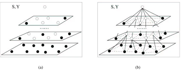
(a) (b)
Figure 4: (a) The initial setting of DHMRFs with a set of nodes that are arranged in multi-layers. Filled circles denote leaf nodes or elements and empty circles denote inner blocks of a webpage; (b) An instance of DHMRFs denoted by S and Y. Vertical edges are selected by posterior probabilities p(s|x). Dotted lines represent the 2D neighborhood system between nodes at the same layer.
values from a finite discrete label space
Y
i. Here, capitalized characters denote random variables and corresponding lower cases are their instances or configurations, for example, y is a label assignment and yi∈Y
iis one component label. A state of the system is the pairing of a model structure and a label assignment, that is,(s,y). Given observations x, Dynamic Hierarchical Markov Random Fields (DHMRFs) define a conditional probability distribution p(s,y|x)of structure s and label assignment y. An example is shown in Figure 4, where the left graph is the initial setting of DHMRFs with a set of nodes that are arranged in multi-layers and the right is an instance of the dynamic model. Let the energy of the system being at the state(s,y)be E(s,y,x), then the probability of the system being at this state isp(s,y|x) = 1
Z(x)exp{−E(s,y,x)}.
This is a Boltzmann distribution with the temperature T =1, and our model is one type of exponen-tial random graph model (Robins et al., 2006). Since the system consists of two parts, the energy is also from two parts. We explain them as follows:
Structure Model: Let sil be an indicator variable to denote the connectivity between node i and another node l, which is at the direct above level. sil equals to 1 if node i connects to node l; otherwise it is 0. Here, leaf nodes can be at any level except the root node that is taken as a default node for an entire page. For leaf nodes, no child is allowed. We call the parent-child connection vertical connection. To retain the computational advantage of tree-structured models, each node is allowed to have only one parent in a particular structure s. We will use sv to denote the set of vertical connections. With the aforementioned definitions of L and Nd, we get sv=∪Ld−=11{sil: 0≤ i<Ndand 0≤l<Nd−1}.
i connects to node j; otherwise, it is 0. Let’s denote the set of horizontal connections by sh, then sh=∪Ld−=01{ni j: 0≤i,j<Ndand i6= j}. Here, we assume that the variables ni jare independent of sil and can be determined using some spatial ordering method. This assumption holds in applications such as web data extraction and image processing. As position information is encoded in each node, deterministic spatial ordering can decide the neighborhood system among a set of nodes. In theory, the horizontal neighborhood system can be arbitrary. We consider the 2D cases (Zhu et al., 2005), that is, each node is horizontally connected to all the nearest surrounding nodes in a 2D plane.
With the structure model, the first part of the energy when the system is at the state(s,y)is
E1(s,y,x) =
∑
kµk
∑
i jlsilsjlni jgk(i,j,l,x),
where a triple(i,j,l)denotes a particular position in the dynamic model. A position can be a time interval in time series or a region of space in random fields. Here, i and j are two nodes at the same layer and l is a node at the direct above layer. gkare feature functions defined on the three nodes at position(i,j,l), and µkare their weights.
Class Label Model: A sample s from the structure model defines a Hierarchical Conditional Random Field, which has been defined in Section 3.4.2. Letαyi be an indicator variable to denote the variable Yitaking the class label y. Then, the second part of the energy when the system is at the state(s,y)is
E2(s,y,x) =
∑
k
λk
∑
i jlsilsjlni j
∑
yi,yj,ylαyi
i α yj
j α yl
l fk(yi,yj,yl,x),
where fk are feature functions defined on the labels yi, yj, and yl at position(i,j,l), andλkare their weights.
Although conditional models take observations as global conditions, when defining feature func-tions they need to know the “focused observafunc-tions” at a particular position. For example, in linear-chain CRFs (Lafferty et al., 2001) the observation at time t is among the focused observations when defining feature functions related to the label yt. In general, let t be a position and xt be the set of focused observations at that position. The mapping functionζ: t→xt defines the focused observa-tions for each position. In generative models (Todorovic and Nechyba, 2005), the mapping function is defined to determine the observations generated by the states at a particular position. Moreover, an additional constraint ∀t 6=s,xt∩xs= /0 is also set due to their independence assumption that observations at different positions are conditionally independent given the states at those positions. In conditional models, however, there is no such constraint. The mapping function can be determin-istic or stochastic. We assume it to be determindetermin-istic in this paper. Now, all feature functions take an additional argumentζ, that is, the feature functions are gk(i,j,l,x,ζ)and fk(yi,yj,yl,x,ζ).
Taking E1and E2together, we get the joint distribution of s and y
p(s,y|x) = 1
Z(x)exp
∑
kµk∑i jlsilsjlni jgk(i,j,l,x,ζ)+
∑kλk∑i jlsilsjlni j∑yi,yj,ylα
yi
i α yj
j α yl
l fk(yi,yj,yl,x,ζ)
,
4.2 Parameter Estimation and Labeling
Let Θ ={µ1,µ2, . . .;λ1,λ2, . . .} denote the whole set of the model’s parameters, and let D = {(xi,yie)}K
i=1denote the set of training data, where xi is a sample and yie are observed labels. We consider the general case with both hidden hierarchical structure s and hidden labels yh. For ex-ample, in web data extraction only the labels of leaf nodes are observable and both the hierarchical structures and the labels of inner nodes are hidden. So the log-likelihood of the data is incomplete
L(Θ) =
K
∑
i=1
log p(yie|xi) =
K
∑
i=1 log(
∑
s,yh
p(s,yh,yie|xi)).
This function does not have a closed-form solution because of the marginalization taking place within the logarithm. In the following, we derive a lower bound of the log-likelihood, or equivalently an upper bound of the negative log-likelihood. Then, contrastive divergence learning (Hinton, 2002) is applied as an approximation.
Let q(s,yh|ye,x) be an approximation of the true distribution p(s,yh|ye,x). With a little abuse of notations, we will use q(s,yh)to denote q(s,yh|ye,x). We also ignore the summation operator in the log-likelihood during the following derivations, as there is no essential difference between one sample and a set of independently and identically distributed (IID) samples. The optimal approxi-mation is the distribution that has the minimum Kullback-Leibler divergence between q(s,yh)and p(s,yh|ye,x). The KL divergence is defined as KL(q||p) =∑s,yhq(s,yh)log
q(s,yh)
p(s,yh|ye,x).
Take p(s,yh|ye,x) = p(s,yh,ye|x)/p(ye|x)into the above equation and use the non-negativity of KL divergence, we get a lower bound of the log-likelihood
log p(ye|x)≥
∑
s,yhq(s,yh)[log p(s,yh,ye|x)−log q(s,yh)].
Equivalently,
L
(Θ),∑s,yhq(s,yh)[log q(s,yh)−log p(s,yh,ye|x)]is an upper bound of theneg-ative log-likelihood−L(Θ). By analogy with statistical physics, the upper bound, which is actually a KL divergence, can be expressed as the difference of two free energies:
L
(Θ) =F0−F∞, where the first term is the free energy when we use data distribution with observable labels clamped to their values, and the second F∞=−log Z(x)is the free energy when we use model distribution with all variables free.Now, the problem is to minimize the upper bound. The derivatives of
L
(Θ)with respect toλk are∂
L
(Θ)∂λk
= ∂
∂λk
h−log p(s,yh,ye|x)iq(s,yh)
=−
∑
i jl
hsilsjlni jiq(s,yh)
∑
yi,yj,yl
hαyi
i α yj
j α yl
l iq(s,yh)fk(yi,yj,yl,x,ζ)−
∂F∞
∂λk
=−
∑
i jl
ni jhsilsjliq(s,yh)
∑
yi,yj,yl
hαyi
i α yj
j α yl
l iq(s,yh)fk(yi,yj,yl,x,ζ)−
∂F∞
∂λk
, (1)
Similarly, the derivatives of
L
(Θ)with respect to µk are∂
L
(Θ)∂µk
=−
∑
i jl
ni jhsilsjliq(s,y
h)gk(i,j,l,x,ζ)−
∂F∞ ∂µk
. (2)
In (1) and (2), the derivatives of the equilibrium free energy F∞ are intractable in the case of Dynamic Hierarchical Markov Random Fields. However, by viewing the equilibrium distribution as the distribution of a Markov chain at time t =∞starting with data distribution, Markov chain Monte Carlo (MCMC) method can be used to reconstruct an approximation distribution qi(s,yh,ye) within several steps. This is the basic idea of contrastive divergence learning (Hinton, 2002). Now, the upper bound is approximated by
L
(Θ)=F0−F∞≈F0−Fi=KL(q0||p)−KL(qi||p),CFiApp,
where q0=q(s,yh)is optimized with observable labels clamped to their values, and qi(s,yh,ye)is optimized with all variables free starting with q0. As shown by Hinton (2002), CFiApp, known as contrastive divergence, is non-negative. But since Fi≥F∞, there is no guarantee that it is still an upper bound. Some analyses of contrastive divergence learning (Yuille, 2004; Carreira-Perpinan and Hinton, 2005) have been carried out. In the sequel, we will set i=1.
Now, the derivatives of CF1Appwith respect to the model’s parameters are as in (1) and (2) but with the derivatives of F∞replaced by
−
∑
i jlni jhsilsjliq1
∑
yiyjylhαyi
i α yj
j α yl
l iq1fk(yi,yj,yl,x,ζ)and −
∑
i jl
ni jhsilsjliq1gk(i,j,l,x,ζ)
respectively.
Generally, stochastic sampling is quite time demanding in constructing q1. In contrast, the deterministic mean field variant (Welling and Hinton, 2001) is more efficient. An extension to the combination of a general deterministic variational approximation and contrastive divergence is studied by Welling and Sutton (2005). The learning procedure consists of two phases—wake phase and sleep phase. Wake phase is to optimize q0 and sleep phase is to optimize q1. We address the wake phase first.
Assume q0can be factorized as q0=q(s,yh) =q(s)q(yh), and we get
KL(q0||p) =−hlog p(s,yh,ye|x)iq0−H(q(s))−H(q(yh)), (3)
Let µil be the probability of node i being connected to node l, and myi be the probability of variable Yibeing at state y. As we assume variables ni j are determined independent of sil, the mean field distributions2are
q(s) =
∏
il
[µil]sil and q(y
h) =
∏
iy[myi]αyi.
Substitute the above distributions into (3) and keep q(yh)fixed, then we get
KL(q0||p) =−hlog p(s,yh,ye|x)iq0−H(q(s)) +c,
where c is a constant. Let the derivative over µilequal zero, and we get
µil∝exp
∑
kµksil∑jhsjliq(s)ni jgk(i,j,l,x)+
∑kλksil∑jhsjliq(s)ni j∑y1,y2,y3hα
y1
i α y2
j α y3
l iq(yh)fk(y1,y2,y3,x,ζ)
. (4)
Normalization will lead to the desired probabilities µil. Similarly, keep q(s)fixed and we get
KL(q0||p) =−hlog p(s,yh,ye|x)iq0−H(q(yh)) +c
0,
where c0is another constant. Let the derivative over myi equal zero, and we get
myi ∝exp
∑
kλk
∑
jly1y2
ni jhsilsjliq(s)hαyj1α y2
l iq(yh)fk(y,y1,y2,x,ζ)+
ni jhsjlsiliq(s)hαy1
j α y2
l iq(yh)fk(y1,y,y2,x,ζ)+
njlhsjisliiq(s)hαyj1α y2
l iq(yh)fk(y1,y2,y,x,ζ)
. (5)
Note that since sil andαyi are all indicator variables, their expectations are the marginal prob-abilities µil and myi respectively. Also, because of the na¨ıve mean field assumption of q(s) and q(yh), the expectations of the product of the indicator variables is the product of their corresponding marginal probabilities, that is,hsilsjliq(s)=µilµjl, hsjisliiq(s)=µjiµli, hαyj1α
y2
l iq(yh)=m
y1
j m y2
l , and hαy1
i α y2
j α y3
l iq(yh)=m
y1 i m y2 j m y3 l .
Equations (4) and (5) are a set of coupled equations, also known as mean field equations. These equations are iteratively solved for a fixed point solution. Intuitively, parameters µil are updated by expected contributions from possible parents and neighbors, and similar for myi. In (4) and (5), structure parameters µil depend on class label assignments, and myi depend on expected structure connectivity. Thus, model structure selection is integrated with label assignment during the infer-ence.
Now, we have presented a mean field approximation of the wake phase. To finish the sleep phase, the same mean field equations are enforced by coordinate descent alternating between ob-servable variables Ye and hidden variables S and Yh. When first optimizing (5) for Ye, the initial distribution of hidden variables are set as the optimal distribution at the end of wake phase. Then, take the optimal distribution of the former step as initial distribution of Yeand optimize (4) and (5) to get an approximate distribution of hidden variables. For wake phase, initial distributions can be random and convergence is arrived at. But for sleep phase, a few steps are required to guarantee the improvement of CF1App.
Thus, all the terms in (1), (2), (4), and (5) can be calculated. The whole parameter estimation algorithm is as follows. First, apply (4) and (5) to iteratively compute the marginal probabilities of both wake and sleep phases. With the marginal probabilities, CF1Appand its derivatives with respect to model parameters are calculated. Then, gradient-based optimization algorithms are applied to update model parameters. Here, we use the limited memory quasi-Newton method (Liu and No-cedal, 1989). The learning procedure is iterated until the relative change of CF1Appis below some threshold. Although no guarantee exists that global optimization will be achieved, empirical studies show that this algorithm performs well.
For labeling a testing example, Equations (4) and (5) are iteratively solved with all variables free for a fixed point solution. At the end of convergence, the maximum a posterior model structure (a tree) is constructed from the probabilities µilby dynamic programming, and the most likely label assignments are found from the marginal probabilities myi.
5. Implementation Details and Experimental Setup
Our experiments consist of two parts. The first part is to evaluate the performance of integrated web data extraction models compared with existing decoupled methods. The second part is to evaluate Dynamic Hierarchical Markov Random Fields (DHMRFs) compared with fixed-structured hierarchical models and Dynamic Trees (Williams and Adams, 1999). All the experiments are carried out on a real-world web data extraction task—production information extraction. In this section, we present the implementation details and the setup of our experiments. Results will be reported in the next two sections.
5.1 Features
As conditional models, DHMRFs and HCRFs can incorporate any useful feature for web data ex-traction. In this section, we present the types of features used in our experiments. As we shall note some of the features have been used in some existing extraction methods. However, they were mainly used as heuristic rules.
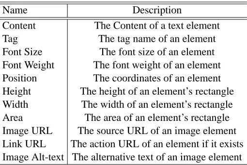
5.1.1 FEATURES OFELEMENTS
For each element, we extract both content and visual features as listed in Table 1. All the features can be obtained through rendering a page. Previous work (Zhai and Liu, 2005; Zhu et al., 2005; Zhao et al., 2005; Gatterbauer et al., 2007) has shown the effectiveness of visual features for webpage analysis and information extraction.
5.1.2 FEATURES OFBLOCKS
The features of inner blocks are aggregations of their children’s features. These features can be extracted via a bottom-up procedure starting from leaf nodes (or elements), such as the number of the children having a particular feature and the presence of a feature or a simultaneous presence of several features among the children. We also compute the following distances for each block to exploit the regularity of similar data records in a page.
sub-Name Description
Content The Content of a text element Tag The tag name of an element Font Size The font size of an element Font Weight The font weight of an element Position The coordinates of an element Height The height of an element’s rectangle Width The width of an element’s rectangle Area The area of an element’s rectangle Image URL The source URL of an image element Link URL The action URL of an element if it exists Image Alt-text The alternative text of an image element
Table 1: The content and visual features of each element.
trees. Although the time-complexity of computing this distance could be high, we can substantially reduce the computation with some heuristics. For example, if the depth difference of two sub-trees is too large, they are not likely to be similar and this computation is not necessary. Once we have computed the tree distances, we can use some thresholds to define boolean-valued feature functions. For example, if the tree distance of two adjacent blocks is not more than 0.2, they are both likely to be data records.
Shape Distance and Type Distance Features: we also compute the shape distance and type distance (Zhao et al., 2005) of two blocks to exploit their similarity. For shape distance, we use the same definition of shape codes and the same calculation method as in the work (Zhao et al., 2005). To compute the type distance of two blocks, we define the following types for each element:
IMAGE: the element is an image.
JPEG IMAGE: the image element that is also a jpeg picture.
CODED IMAGE: the image element whose source URL contains at least three succeeding numbers, such as “/products/s thumb/eb04iu 0190893 200t1.jpg”.
TEXT: the element has text content.
LINK TEXT: the text element that contains an action URL.
DOLLAR TEXT: the text element that contains at least one dollar sign. NOTE TEXT: the text element whose tag is “input”, “select” or “option”. NULL: the default type of each element.
After defining each element’s type code, a block’s type code is defined as a sequence of the type codes of its children. As in the work by Zhao et al. (2005), multiple consecutive occurrences of each type are compressed to one occurrence. The edit distance of type codes is the type distance of two blocks.
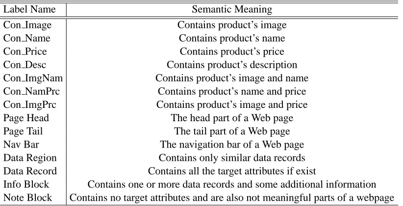
Label Name Semantic Meaning Con Image Contains product’s image
Con Name Contains product’s name
Con Price Contains product’s price Con Desc Contains product’s description Con ImgNam Contains product’s image and name Con NamPrc Contains product’s name and price Con ImgPrc Contains product’s image and price Page Head The head part of a Web page Page Tail The tail part of a Web page Nav Bar The navigation bar of a Web page Data Region Contains only similar data records Data Record Contains all the target attributes if exist
Info Block Contains one or more data records and some additional information Note Block Contains no target attributes and are also not meaningful parts of a webpage
Table 2: Label spaces of inner variables for product information extraction.
function appears sparsely in the training set, smoothing techniques can be used to avoid over-fitting. Here, we use the spherical Gaussian prior to penalize the log-likelihood function during learning.
5.1.3 GLOBALFEATURES
As described in the introduction, data records in the same webpage are always related. Based on work by Zhai and Liu (2005), we try to align the elements of two adjacent blocks in the same page and extract some global features to help attribute labeling.
For two neighboring blocks, we use the partial tree-alignment algorithm (Zhai and Liu, 2005) to align their elements. An alignment is discarded if most of the elements are not aligned. For successful alignments, the following feature is extracted.
Repeated elements are less informative: this feature is based on the observation that repeated elements in different records are more likely to be less useful, while important information such as the name of a product is not likely to repeat in the same webpage. For example, the “Add to cart” button appears in both data records as in Figure 1(a), but each record has a unique name. Currently, we just denote whether an element is repeated in different records. More complex measures like information entropy can be easily adopted. An example feature function can be defined as: if the element xi repeatedly appears in the aligned records, it will be more likely to be labeled as Note or noise.
5.2 Label Spaces
product information extraction, the leaf label space consists of Name, Image, Price, Description, and Note. Note is used to describe the data we are not interested in.
The inner label space can be partitioned into an object-type independent part and an object-type dependent part. We explain how to define these two parts in turn:
Object-type Independent Labels: Since we want to extract data from webpages, the labels Page Head, Page Tail, Nav Bar, and Info Block are naturally needed to denote different parts of a webpage. The labels Data Record and Data Region are also required for detecting data records. The label Note Block is also required to denote blocks that do not contain any meaningful information, such as the attributes to be extracted and the head, tail or navigation bar of a webpage. All these labels are general to any web data extraction problem, and they are independent of any specific object type.
Object-type Dependent Labels: Between data record blocks and leaf blocks, there are inter-mediate blocks on a vision-tree. So, we must define some interinter-mediate labels between Data Record and the labels in the leaf label space. These labels are object-type dependent because intermediate blocks contain some object specific attribute values. A natural method is to use the combinations of the attributes to define intermediate labels. Of course, if we use all the possible combinations, the label space could be too large. We can discard unimportant combinations by considering the co-occurrence frequencies of their corresponding attribute values in the training data. The object-type dependent labels in product information extraction are listed in Table 2 with the format Con *.
5.3 Data Sets
We set up two general data sets with randomly crawled product webpages. The list data set (LDST) contains 771 list pages and the detail data set (DDST) contains 450 detail pages. All the pages are parsed by VIPS and are hierarchically labeled, that is, every block in the parsed vision-trees is labeled. We use 200 list pages and 150 detail pages to learn the parameters of different models. The remaining pages (571 list pages and 300 detail pages) are used for testing. For each product item, we want to extract four attributes—Name, Image, Price, and Description.
For the training data, the detail pages are from 61 web sites and the list pages are from 81 web sites. The number of web sites that are found in both list and detail training data is 39. Thus, in total the training pages are taken from 103 different web sites. Totally, 58 unique templates are presented in the list training pages and 61 unique templates are presented in the detail training pages. For testing data, Table 3 shows the number of unique web sites where the pages come from and the number of different templates presented in these data. For example, the pages in LDST are from 167 web sites, of which 78 are found in list training data and 52 are found in detail training data. The number of web sites that are found in both list and detail training data is 34. Similar interpretation applies to other numbers in the table. Thus, totally 71 list page web sites and 263 detail page web sites are not seen in the training data. For templates, 83 list page templates and 208 detail page templates are not seen the training data. For different templates, the number of documents varies. In LDST, most of the templates have 2 to 5 documents. In DDST, pages from different web sites typically have different templates and thus most templates have 1 document.
5.4 Evaluation Metrics
Data Sets LDST DDST #Web Site 167 (78/52/34) 268 (2/3/0) #Template 140 (57/0/0) 212 (0/4/0)
Table 3: Statistics of the data sets.
attributes of one object, and does not contain any attributes of other objects. A correct data record could tolerate (miss or contain) some non-important information like “Add to Cart” button.
For attribute labeling, the performance on each attribute is evaluated by Precision (the per-centage of returned elements that are correct), Recall (the perper-centage of correct elements that are returned), and their harmonic mean F1. We also use two comprehensive evaluation criteria:
Block Instance Accuracy (Blk IA): the percentage of data records of which the key attributes (Name, Image, and Price) are all correctly labeled.
Average F1 (Avg F1): the average of F1 values of different attributes.
6. Evaluation of Integrated Web Data Extraction Models
In this section, we report the evaluation results of integrated web data extraction models compared with decoupled models. The results demonstrate that integrated extraction models can achieve significant improvements over decoupled models in both record detection and attribute labeling. We also show the generalization ability of the integrated extraction models.
6.1 Methods
We build the baseline methods by sequentially combining the record detection algorithm DEPTA (Zhai and Liu, 2005) and 2D CRFs (Zhu et al., 2005). For detail pages, which DEPTA cannot deal with, we first detect the main data block using the method by Song et al. (2004) and then use 2D CRFs to perform attribute labeling on the detected main block. For the integrated extraction model, a webpage is first segmented by VIPS to construct a vision-tree and then HCRFs are used to detect both records and attributes on the vision-tree. Note that all the HCRFs evaluated in this section are the model in Figure 3(b). The evaluation results of another HCRFs, which are slightly better, are presented in Section 7.
To see the effect of the global features in Section 5.1.3, we also evaluate an HCRF model that does not use these global features. We denote this model by H NG (without global features). Similarly, we evaluate two 2D CRF models in the baseline methods. As in the work of Zhu et al. (2005), a basic 2D CRF model is set up with only the basic features (see Table 1) when labeling each detected data record. Another 2D CRF model is set up with both the basic features and the global features. We denote the basic model by 2D CRF and denote the other model by 2D G. For 2D G, we first cache all the detected records from one webpage and then extract the global features. As there is no tree structure here, the alignments are based on the elements’ relative positions in each record.
attribute labeling, we also evaluate two HCRF models with and without the global features. These two models are denoted by H S and H SNG respectively.
For all the HCRF models, we use 200 list pages and 150 detail pages together to learn their parameters. We use the same 200 list pages to train a 2D CRF model for extraction on list pages, and use the same 150 detail pages to train another 2D CRF model for extraction on detail pages. The reason for training two models for list and detail pages separately is that, for a 2D CRF model, the features and parameters for list and detail pages are quite different and a uniform model cannot work well. In the training stage, all of the algorithms converge quickly, within 20 iterations.
6.2 Results and Discussions
We compare our approach with DEPTA (Zhai and Liu, 2005) on LDST for data record detection. The running results of DEPTA on our data set are kindly provided by its authors. DEPTA has a similarity threshold, and it is set at 60% in this experiment. Some simple heuristics are also used in DEPTA to remove some noise records. For example, a data region that is far from the center or contains neither image nor dollar sign is removed.
6.2.1 RECORDDETECTION
The results of record detection are shown in Table 4. We can see that both HCRF and H NG significantly outperform DEPTA in recall, improved by 8.1 points, and precision, improved by 7.5 points. The improvements come from two parts:
Advanced data representation and more features: in our model, we incorporate more features such as content features and shape distance and type distance features than DEPTA. We also adopt an advanced representation of webpages—vision-trees which have been shown to outperform tag-tree representation(Cai et al., 2004). As we can see from Table 4, H SNG and H S outperform DEPTA, and we gain about 2 points in precision, 7.3 points in recall, and 4.6 points in F1.
Incorporation of semantics during record detection: DEPTA just detects the blocks with reg-ular patterns (i.e., regreg-ular tree structures) and does not take semantics into account. Thus, although some heuristics are used to remove some noise blocks, the results still contain blocks that are not data records or just parts of data records. In contrast, our approach integrates attribute labeling into block detection and can consider semantics during detecting data records. So, the blocks de-tected are of better quality and are more likely to be data records. For instance, a block containing a product’s name, image, price and some descriptions is almost certain to be a data record, but a block containing only irrelevant information is unlikely to be a data record. The lower precisions of H SNG and H S demonstrate this. When not considering the semantics of the elements, H SNG and H S extract more noise blocks compared with H NG or HCRF, so the precisions of record detection decrease by 5.5 points and the overall F1 measures decrease by 3.2 points.
6.2.2 ATTRIBUTELABELING
Models H SNG H S H NG HCRF DEPTA P 0.904 0.904 0.959 0.959 0.884 R 0.921 0.921 0.930 0.930 0.849 F1 0.912 0.912 0.944 0.944 0.866
Table 4: Record detection results of different methods on LDST.
Data Sets LDST DDST
Models H SNG H S H NG HCRF 2D CRF 2D G HCRF 2D CRF Name 0.836 0.860 0.880 0.911 0.763 0.851 0.835 0.398 P Image 0.901 0.905 0.952 0.966 0.842 0.838 0.978 0.546 Price 0.906 0.903 0.959 0.963 0.913 0.915 0.986 0.809 Desc 0.783 0.766 0.792 0.788 0.769 0.779 0.663 0.588 Name 0.851 0.875 0.854 0.882 0.735 0.822 0.761 0.398 R Image 0.917 0.921 0.924 0.936 0.811 0.809 0.892 0.546 Price 0.922 0.919 0.930 0.933 0.879 0.883 0.899 0.809 Desc 0.797 0.780 0.768 0.764 0.741 0.752 0.604 0.395 Name 0.843 0.867 0.867 0.896 0.749 0.836 0.796 0.398 F1 Image 0.909 0.913 0.938 0.951 0.826 0.823 0.933 0.546 Price 0.914 0.911 0.944 0.948 0.896 0.899 0.940 0.809 Desc 0.790 0.773 0.780 0.776 0.755 0.765 0.632 0.473 Avg F1 0.864 0.866 0.882 0.893 0.807 0.831 0.825 0.556 Blk IA 0.789 0.816 0.856 0.890 0.669 0.751 0.817 0.231
Table 5: Attribute labeling results of different methods on both LDST and DDST, where Desc stands for Description.
Attribute labeling benefits from good quality records: one reason for this better performance is that attribute labeling can benefit from the good results of record detection. For example, if a detected record is not a data record or misses some important information such as Name, attribute labeling will fail to find the missed information or will find some incorrect information. So, H SNG outperforms 2D CRF and H S outperforms 2D G. Of course the achievements of H SNG and H S may also come from the incorporation of long distance dependencies, which will be discussed later. Global features help attribute labeling: another reason for the improvements in attribute la-beling is the incorporation of the global features as in Section 5.1.3. From the results, we can see that when considering global features, attribute labeling is more accurate. For example, 3.4 points are gained in block instance accuracy by HCRF compared with H NG, and H S achieves 2.7 points in block instance accuracy compared with H SNG. For the two baseline methods, compared with 2D CRF, which uses only the features of the elements in each detected record, more than 8 points are gained in block instance accuracy by 2D G, which incorporates the global features.
promising results while 2D CRFs perform poorly on detail pages. This is because, for a detected record, 2D CRFs put its elements in a two-dimensional grid and long distance interactions cannot be incorporated in the flat model, due to the first-order Markov assumption. In contrast, HCRF models can incorporate dependencies at various levels and thus incorporate long distance dependencies. For detail pages, as there is no record detection, H SNG and H S are not applicable here. There are no global features either, so we just list the results of HCRF and 2D CRF in Table 5.
The quite different performance of 2D CRFs on list and detail pages says the same thing about the effectiveness of long distance dependencies. For list pages, the inputs are data records, which always contain a small number of elements. In this case, 2D CRFs can effectively model the depen-dencies of the attributes and achieve reasonable accuracy. Note that the results on detail pages are achieved without any pre-processing to remove noise elements. Empirical studies show that some appropriate pre-processing can improve the performance significantly on detail pages.
6.3 Generalization Ability
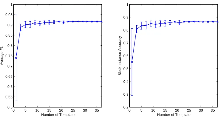
We report some empirical results to show the generalization ability of the integrated web data ex-traction models. We randomly pick 37 templates from LDST and for each template we collect 5 webpages for training and 10 webpages for testing. We randomly select N(N=1,2,3,· · ·,37)
templates together with their training pages as training data, and test the model on all the testing webpages of the 37 templates. For each N, we run the integrated HCRFs 10 times and take the average as the final results. Figure 5 shows the average F1 and block instance accuracy against different N. We can see that the integrated extraction models converge very quickly. As the number of templates increase in the training data, the extraction accuracy becomes higher and the variances become smaller. The strong generalization ability to unseen templates is mainly due to the very general and robust visual features we are using in our models. For different templates, although the low-level HTML codes or HTML tag trees are quite different, the visual layout and visual features they use are usually common. Thus, we can learn a robust model from a small set of templates and generalize well to unseen templates. Section 7.3 presents another set of results that show the generalization ability to unseen templates.
7. Evaluation of Dynamic Hierarchical Markov Random Fields
In this section, we report the evaluation results of Dynamic Hierarchical Markov Random Fields compared with fixed-structured hierarchical models and Dynamic Trees. Results show that DHM-RFs can (at least partially) overcome the blocky artifact issue in diverse web data extraction. We also present some empirical studies about the learning algorithm of DHMRFs.
7.1 Models
0 5 10 15 20 25 30 35 0.5
0.55 0.6 0.65 0.7 0.75 0.8 0.85 0.9 0.95 1
Number of Template
Average F1
0 5 10 15 20 25 30 35
0.2 0.3 0.4 0.5 0.6 0.7 0.8 0.9 1
Number of Template
Block Instance Accuracy
Figure 5: The left plot is the mean and variance of the Average F1 and the right plot is the mean and variance of the Block Instance Accuracy.
label assignment. We will use HCRF and HCRF+ to denote the two HCRF models in Figure 3(b) and 3(c) respectively.
To apply DHMRFs and D-Trees, initial configuration of the model structure must be carried out first. Basically, we need to initially set the number of layers and the number of nodes at each layer. It may be different for different application domains to set the initial configuration. For image processing, it can be done via sub-sampling or wavelet filtering. For web data extraction, the data are represented as texts, images, buttons, and so on. These atomic information units are more expressive compared to image pixels. There is definitely no benefit to view a webpage as a collection of image pixels and then apply the methods in image processing. Here, we use the same number of layers (and the same number of nodes at each layer) in dynamic models as in the vision-trees. Note that additional nodes can be introduced. For DHMRFs feature functions can be easily defined to consider these nodes, and for D-Trees the part-time-node-employment prior (Adams and Williams, 1999) can be applied to get a sparse structure.
7.2 Extraction Accuracy
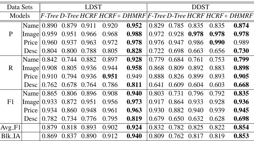
Table 6 shows the extraction accuracy of different models. From the results, we can see that DHM-RFs achieve the highest performance on both data sets. Compared to the fixed HCRF, on LDST about 3 points in Average F1 and about 5 points in Block Instance Accuracy are gained. Compared to the more complex HCRF+, more than 2 points in Average F1 and about 3 points in Block Instance Accuracy are achieved. More specifically, compared to HCRF+, more than 3 points are achieved in both precision and recall on Name, and more than 2 points are achieved on Desc. For Image and Price the improvements are smaller. This is because Image and Price are usually more distinctive than the other attributes. So both models perform quite well. On DDST, the improvements in Name are about 4 points in both precision and recall, and for Description the improvements are about 7 points in both precision and recall. Small improvements are achieved in Image and Price due to the same reason as in list pages.
The improvements demonstrate the merits of DHMRFs. First, DHMRFs can incorporate the two-dimensional neighborhood dependencies among the nodes at the same level, which have been shown to be useful (Zhu et al., 2005). The better performance of HCRF+ compared to HCRF also shows the usefulness of two-dimensional neighborhood dependencies. By dynamically selecting connections between different nodes, DHMRFs can bring together the attributes of the same ob-ject (here, an obob-ject is a product item), and thus the correlation between these attributes can be strengthened. Second, DHMRFs can deal with webpages with intertwined attributes (Zhai and Liu, 2005). For these webpages, the attributes of different objects are intertwined in HTML tag trees. Unaware of semantic labels, the constructed vision-trees also have intertwined attributes. In these cases, fixed-structured HCRFs (both HCRF and HCRF+) cannot correctly detect data records by simply assigning labels to the nodes of a vision-tree. Instead, as structure selection is integrated with labeling in DHMRFs, the dynamic model can properly group the attributes of the same object, and at the same time separate the attributes of different objects with the help of semantic labels. The semantic labels have been shown to be helpful in detecting data records (i.e., groups of attributes) in previous experiments. Note that although intertwined cases are usually fewer than non-intertwined cases, they are not sparse samples in our model. This is because although their edge connections in HTML tag trees are somewhat different from non-intertwined ones, the visual features they share are almost the same. Thus, training samples with or without intertwined cases can teach a good model. In fact, to keep it fair for both dynamic models and fix-structured models, we only provide non-intertwined samples during training.
non-Data Sets LDST DDST
Models F-Tree D-Tree HCRF HCRF+ DHMRF F-Tree D-Tree HCRF HCRF+ DHMRF Name 0.890 0.879 0.911 0.920 0.952 0.829 0.785 0.835 0.835 0.874 P Image 0.959 0.951 0.966 0.968 0.988 0.972 0.928 0.978 0.978 0.978 Price 0.960 0.937 0.963 0.972 0.978 0.976 0.947 0.986 0.990 0.989 Desc 0.804 0.800 0.788 0.805 0.828 0.722 0.698 0.663 0.656 0.730 Name 0.842 0.744 0.882 0.897 0.928 0.779 0.684 0.761 0.753 0.799 R Image 0.908 0.805 0.936 0.944 0.958 0.868 0.809 0.892 0.883 0.898 Price 0.910 0.794 0.936 0.951 0.949 0.888 0.826 0.899 0.893 0.905 Desc 0.762 0.678 0.764 0.786 0.811 0.641 0.609 0.604 0.603 0.668 Name 0.865 0.806 0.896 0.908 0.940 0.803 0.731 0.796 0.792 0.835 F1 Image 0.933 0.872 0.951 0.956 0.973 0.917 0.864 0.933 0.928 0.936 Price 0.934 0.860 0.948 0.961 0.963 0.930 0.882 0.940 0.939 0.945 Desc 0.782 0.734 0.776 0.795 0.819 0.679 0.650 0.632 0.628 0.698 Avg F1 0.879 0.818 0.893 0.902 0.924 0.832 0.782 0.825 0.822 0.854 Blk IA 0.869 0.837 0.890 0.912 0.940 0.809 0.762 0.817 0.819 0.853
Table 6: Extraction accuracy on LDST and DDST, where Desc stands for Description.
intertwined cases well. The results also show that the directed tree models can perform well on our data sets, but are inferior to HCRFs.
7.3 Extraction Accuracy on Unseen Templates
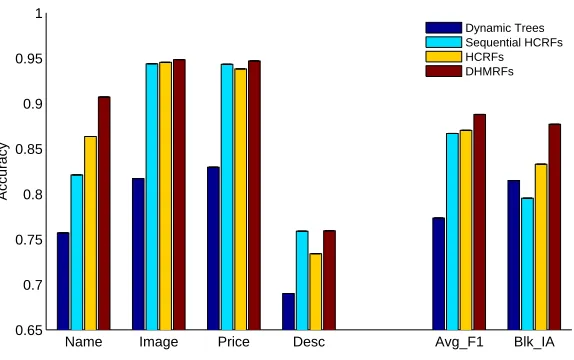
For detail pages, since only a small number (i.e., 4) of templates in the testing data are seen in the training data, the results on webpages generated from unseen templates do not change much. Here, we only report the results on list pages. In total, LDST has 83 templates that are not seen in the training data. We select out all the pages with unseen templates, the total number being 190. Figure 6 shows the results of our models on these webpages. The overall performance is still very promising although it is lower than that on the whole set of webpages. Generally, the Dynamic Hierarchical Markov Random Fields always outperform all the other models. The integrated HCRFs outperform the sequential HCRFs, which take record detection and attribute labeling as two separate steps as described in Section 6.1. Dynamic Trees achieved the worst results due to the same reason of a less discriminative power in structure selection.
7.4 Fitness of Model Structure
Name Image Price Desc Avg_F1 Blk_IA 0.65
0.7 0.75 0.8 0.85 0.9 0.95 1
Accuracy
Dynamic Trees Sequential HCRFs HCRFs DHMRFs
Figure 6: The performance of Dynamic Trees, Sequential HCRFs, HCRFs, and DHMRFs on the webpages whose templates are not presented in the training data. From left to right, the first four groups of the columns are the F1 of different attributes.
model have higher posterior probabilities. Another observation is that the distribution of samples from DDST is more disperse than that of the samples from LDST. The reason is that in list pages the attributes of an object always concentrate into small clusters, while they can scatter anywhere in detail pages.
7.5 Study about the Inference Algorithm
Figure 7(b) shows the change of average contrastive divergence with respect to iteration numbers in the learning of DHMRFs. To initialize the algorithm, at the wake phrase myi are set to a uniform distribution plus a Gaussian noise with zero mean and variance 0.01, and µil are set to a random distribution. The model weights are initialized to zero. We can see that before 7 iterations average contrastive divergence decreases stably. And after 7, slight disturbances appear. But as for extraction accuracy, marginal changes occur (no more than 0.5 point in Block Instance Accuracy). Thus, the learning algorithm is quite stable. All the above results are achieved at iteration 7. The same initialization is used in labeling, and by running both learning and labeling many times, we observe that the algorithm is insensitive to the random initialization. Since the mean field equations are locally calculated and their update can typically converge within 5 iterations, both the learning and labeling are efficient.
8. Conclusions and Future Work
−200 −180 −160 −140 −120 −100 −80 −60 −40 −20 0 −200
−180 −160 −140 −120 −100 −80 −60 −40 −20 0
Fixed Structure
MAP Dynamic Structure
(a)
0 2 4 6 8 10 12 14
40 60 80 100 120 140 160 180 200 220
Epoch Number
Average Contrastive Divergence
(b)