Minimal Nonlinear Distortion Principle for Nonlinear Independent Component Analysis

Minimal Nonlinear Distortion Principle for Nonlinear Independent

Component Analysis

Kun Zhang KZHANG@CSE.CUHK.EDU.HK

Laiwan Chan LWCHAN@CSE.CUHK.EDU.HK

Department of Computer Science and Engineering The Chinese University of Hongkong

Hong Kong

Editor: Aapo Hyv¨arinen

Abstract

It is well known that solutions to the nonlinear independent component analysis (ICA) problem are highly non-unique. In this paper we propose the “minimal nonlinear distortion” (MND) principle for tackling the ill-posedness of nonlinear ICA problems. MND prefers the nonlinear ICA solution with the estimated mixing procedure as close as possible to linear, among all possible solutions. It also helps to avoid local optima in the solutions. To achieve MND, we exploit a regularization term to minimize the mean square error between the nonlinear mixing mapping and the best-fitting linear one. The effect of MND on the inherent trivial and non-trivial indeterminacies in nonlinear ICA solutions is investigated. Moreover, we show that local MND is closely related to the smooth-ness regularizer penalizing large curvature, which provides another useful regularization condition for nonlinear ICA. Experiments on synthetic data show the usefulness of the MND principle for separating various nonlinear mixtures. Finally, as an application, we use nonlinear ICA with MND to separate daily returns of a set of stocks in Hong Kong, and the linear causal relations among them are successfully discovered. The resulting causal relations give some interesting insights into the stock market. Such a result can not be achieved by linear ICA. Simulation studies also verify that when doing causality discovery, sometimes one should not ignore the nonlinear distortion in the data generation procedure, even if it is weak.

Keywords: nonlinear ICA, regularization, minimal nonlinear distortion, mean square error, best

linear reconstruction

1. Introduction

Independent component analysis (ICA) is a popular statistical technique aiming to recover indepen-dent sources from their observed mixtures, without knowing the mixing procedure or any specific knowledge of the sources (Hyv¨arinen et al., 2001; Cardoso, 1998; Cichocki and Amari, 2003). In the case that the observed mixtures are a linear transformation of the sources, under weak assump-tions, ICA can recover the original sources with the trivial permutation and scaling indeterminacies. Linear ICA is currently a popular method for blind source separation (BSS) of linear mixtures.

However, nonlinear ICA does not necessarily lead to nonlinear BSS. In Hyv ¨arinen and Pa-junen (1999), it was shown that solutions to nonlinear ICA always exist and that they are highly non-unique. Actually, one can easily construct a nonlinear transformation of some non-Gaussian independent variables to produce independent outputs. Below are a few examples. Let y1, ...,yn be

indepen-dent. If we use Gaussianization (Chen and Gopinath, 2001) to transform yiinto Gaussian variables ui, any component-wise nonlinear function of U·u, where u= (u1, ...,un)T and U is an orthogonal

matrix, still has mutually independent components. Taleb and Jutten (1999) also gave an example in which nonlinear mixtures of independent variables are still independent. One can see that nonlinear BSS is impossible without additional prior knowledge on the mixing model, since the independence assumption is not strong enough in the general nonlinear mixing case (Jutten and Taleb, 2000; Taleb, 2002).

If we constrain the nonlinear mixing mapping to have some specific forms, the indeterminacies in the results of nonlinear ICA can be reduced dramatically, and as a consequence, nonlinear ICA may lead to nonlinear BSS. For example, in Burel (1992), a parametric form of the mixing trans-formation is assumed known and one just needs to adjust the unknown parameters. The learning algorithms were improved in Yang et al. (1998). By exploiting the extensions of the Darmois-Skitovich theorem (Kagan et al., 1973) to nonlinear functions, a particular class of nonlinear mixing mappings, which satisfy an addition theorem in the sense of the theory of functional equations, were considered in Eriksson and Koivunen (2002). In particular, the post-nonlinear (PNL) mixing model (Taleb and Jutten, 1999), which assumes that the mixing mapping is a linear transformation followed by a component-wise nonlinear one, has drawn much attention.

In practice, the exact form of the nonlinear mixing procedure is probably unknown. Conse-quently, in order to model arbitrary nonlinear mappings, one may need to resort to a flexible non-linear function approximator, such as the multi-layer perceptron (MLP) or the radial basis function (RBF) network, to represent the nonlinear separation system. Almeida (2003) uses the MLP to model the separation system and trains the MLP by information-maximization (Infomax). More-over, the smoothness constraint,1which is implicitly provided by MLP’s with small initial weights and with a relatively small number of hidden units, was believed to be a suitable regularization condition to achieve nonlinear BSS. In Tan et al. (2001), a RBF network is adopted to represent the separation system, and partial moments of the outputs of the separation system are used for regularization. The matching between the relevant moments of the outputs and those of the original sources was expected to guarantee a unique solution. But the moments of the original sources may be unknown. In addition, if the transformation from the original sources to the recovered sources is non-trivial,2this regularization could not help to recover the original sources. Variational Bayesian nonlinear ICA (Lappalainen and Honkela, 2000; Valpola, 2000) uses the MLP to model the non-linear mixing transformation. By resorting to the variational Bayesian inference technique, this method can do model selection and avoid overfitting. If we can have some additional knowledge about the nonlinear mixing transformation and incorporate it efficiently, the results of nonlinear ICA will be much more meaningful and reliable.

Although we may not know the form of the nonlinearity in the data generation procedure, for-tunately, in many cases the nonlinearity for generating natural signals we deal with is not strong. Hence, provided that the nonlinear ICA outputs are mutually independent, we would prefer the so-lution with the estimated data generation procedure of minimal nonlinear distortion (MND). This

1. Following Tikhonov and Arsenin (1977), here we use the term “smoothness” in a very general sense. Often it means that that the function does not change abruptly and/or that it does not oscillate too much.

information can help to reduce the indeterminacies in nonlinear ICA greatly, and moreover, to avoid local optima in the solutions to nonlinear ICA. The minimal nonlinear distortion of the mixing sys-tem is achieved by the technique of regularization. The objective function of nonlinear ICA with MND is the mutual information between outputs penalized by some terms measuring the level of “closeness to linear” of the mixing system. The mean square error (MSE) between the nonlinear mixing system and its best-fitting linear one provides such a regularization term. To ensure that nonlinear ICA results in nonlinear BSS, one may also need to enforce the local MND of the non-linear mapping averaged at every point, which turns out to be the smoothness regularizer exploiting second-order partial derivatives.

MND, as well as the smoothness regularizer, can be incorporated in various nonlinear ICA methods to improve the results. Here we consider two nonlinear ICA methods. The first one is the MISEP method (Almeida, 2003), where the MLP is used to represent the separation system. As regularization is powerful for complexity control in neural networks (Bishop, 1995), the structure of the MLP is not optimized during the learning process, that is, it is fixed. The second one is non-linear ICA based on kernels (Zhang and Chan, 2007a), in which the nonnon-linear separation system is modeled using some kernel methods. We then explain why MND helps to alleviate the ill-posedness in nonlinear ICA solutions, by investigating the effect of MND on trivial and non-trivial indetermi-nacies in nonlinear ICA solutions systematically. Next, we conduct experiments using synthetic data to compare the performance of several nonlinear ICA methods. The results confirm the effec-tiveness of the proposed MND principle to avoid unwanted solutions and to improve the separation performance. Finally, nonlinear ICA with MND is used to discover linear causal relations in the Hong Kong stock market and give encouraging results. We also give experimental results on syn-thetic data, which illustrate that when performing ICA-based causality discovery on the data whose generation procedure involves nonlinear distortion, one should take into account the nonlinear effect in the ICA separation system, even if it is mild.3

2. Nonlinear ICA with Minimal Nonlinear Distortion

In this section we first briefly review the general nonlinear ICA problem, and then propose the minimal nonlinear distortion (MND) principle for regularization of nonlinear ICA.

2.1 Nonlinear ICA

In the nonlinear ICA model, the observed data x= (x1, ...,xn)T are assumed to be generated from a

vector of independent variables s= (s1, ...,sn)T by a nonlinear transformation:

x=

F

(s), (1)

where

F

is an unknown real-valued n-component mixing function. Here for simplicity, we have assumed that the number of observed variables equals that of the original independent variables. The general nonlinear ICA problem is to find a mapping

G

:Rn→Rnsuch that

y=

G

(x)

has statistically independent components. As mentioned in Section 1, the results of nonlinear ICA are highly non-unique. In order to achieve nonlinear BSS, which aims at recovering the original sources si, we should resort to additional prior information or suitable regularization constraints.

2.2 With Minimum Nonlinear Distortion

We now propose the MND principle to restrict the space of nonlinear ICA solutions. As a conse-quence, the ill-posedness of the nonlinear ICA problem is alleviated. Under the condition that the separation outputs yiare mutually independent, this principle prefers the solution with the estimated

mixing transformation ˆ

F

as close as possible to linear.

Now we need a measure of “closeness to linear” of a mapping. Given a nonlinear mapping ˆ

F

, its deviation from the affine mapping A∗, which fits ˆ

F

best among all affine mappings A, is an indicator of its “closeness to linear”, or the level of its nonlinear distortion. The deviation can be measured in various ways. The MSE is adopted here, as it greatly facilitates subsequent analysis. Consequently, the “closeness to linear” of ˆ

F

=

G

−1 _{can be measured by the MSE between}

G

−1

and A∗. We denote this measure by RMSE(θ), whereθdenotes the set of unknown parameters in the

nonlinear ICA system. Let x∗= (x∗

1,···,x∗n)T be the output of the affine transformation from y by

A∗. Let ˜y= [y; 1]. RMSE(θ)can then be written as the MSE between xiand x∗i:

RMSE(θ) = E{(x−x∗)T(x−x∗)}, where (2)

x∗ = A∗˜y,and A∗=arg_Amin E_{(x₋Ay)T(x₋Ay)_}.

Here A∗is a n×(n+1)matrix.4 Figure 1 shows the separation system

G

together with the genera-tion process of RMSE.

(

θ

)

x

1

x

n

y

1

y

n .

. .

. . .

. . . .

.

.

A

*

x

1*

x

n*

v

1

v

n

Figure 1: The separation system

G

(solid line) and the generation of the regularization term RMSE

(dashed line). RMSE=∑ni=1vi2, where vi=xi−x∗i.

With RMSEmeasuring the level of nonlinear distortion, nonlinear ICA with MND can be

formu-lated as the following constrained optimization problem. It aims to minimize the mutual information between outputs, that is, I(y), subject to RMSE(θ)≤t, where t is a pre-assigned parameter. The

La-grangian for this optimization problem is L(θ,λ) =I(y) +λ[RMSE(θ)−t]withλ≥0. To findθ, we

need to minimize

J=I(y) +λRMSE(θ). (3)

The non-negative constantλdepends on the pre-assigned parameter t.

Another advantage of the MND principle is that it tends to make the mapping

G

invertible. In the general nonlinear ICA problem, it is assumed that both

F

and

G

are invertible. But in practice

it is not easy to guarantee the invertibility of the mapping provided by a flexible nonlinear function approximator, like the MLP. MND pushes

G

to be close to a linear invertible transformation. Hence when nonlinearity in

F

is not too strong, MND helps to guarantee the invertibility of the nonlinear ICA separation system

G

.

2.2.1 SIMPLIFICATION OFRMSE

RMSE, given in Eq. 2, can be further simplified. According to Eq. 2, the derivative of RMSE w.r.t.

A∗ is ∂RMSE

∂A∗ =−2E{(x−A∗˜y)˜yT}. Setting the derivative to 0 gives E{(x−A∗˜y)˜yT}=0, which implies

A∗=E_{x˜yT_}[E_{˜y˜yT_}]−1. (4)

We can see that due to the adoption of the MSE, A∗ can be obtained in closed form. This greatly simplifies the derivation of learning rules.

Due to Eq. 4, we have E_{A∗˜y˜yTA∗T_}=E_{x˜yT_}A∗T ,and RMSE then becomes

RMSE = Tr E{(x−A∗˜y)(x−A∗˜y)T}

= Tr E_{xxT₋A∗˜yxT₋x˜yTA∗T+A∗˜y˜yTA∗T_}

= Tr E{xxT−A∗˜yxT₋x˜yTA∗T+x˜yTA∗T} = ₋Tr E_{A∗˜yxT_}+Tr E_{xxT_}

= ₋Tr E_{x˜yT_}[E_{˜y˜yT_}]−1E_{˜yxT_}+const. (5) Since yi are independent from each other, they are uncorrelated. We can also easily make yi

zero-mean. Consequently, E_{˜y˜yT_}=diag_{E(y2

1),E(y22), ...,E(y2n),1}, and RMSEbecomes RMSE = −Tr E{x˜yT} ·[diag{E(y21), ...,E(y2n),1}]−1·E{˜yxT}

+const

= ₋ n

∑

j=1 n

∑

i=1

E2(xjyi) E(y2

i)

+const. (6)

RMSE depends only on the inputs and the outputs of the nonlinear ICA system

G

(θ). Given a form

for

G

, the learning rule for nonlinear ICA with MND is derived by minimizing Eq. 3. Note that

RMSE, given in Eq. 2, is inconsistent with certain scaling properties of the observations x. To avoid

this, one needs to normalize the variance of the observations xithrough preprocessing, if necessary.

2.2.2 DETERMINATION OF THEREGULARIZATIONPARAMETERλ

We suggest initializingλwith a large value λ0 at the beginning of training and decreasing it to a

small constantλcduring the learning process. A large value forλat the beginning reduces the

pos-sibility of getting into unwanted solutions, which may be non-trivial transformations of the original sources si or local optima. As training goes on, the influence of the regularization term is relaxed,

and

G

gains more freedom. Hopefully, nonlinearity will be introduced, if necessary. The choice of

λc depends on the level of nonlinear distortion in the mixing procedure. If the nonlinear distortion

is considerable, we should use a very small value forλcto give the

G

network enough flexibility. In

our experiments, we found that the separation performance of nonlinear ICA with MND is robust to the value ofλcin a certain range. If the variance of the observations xiis normalized, typical values

2.3 Relation to Previous Works

The MISEP method has been reported to solve some nonlinear BSS problems successfully, includ-ing separatinclud-ing a real-life nonlinear image mixture (Almeida, 2005, 2003). Almeida (2003) claimed that the MLP itself may provide suitable regularization for nonlinear ICA. Some means were also used for regularization in the experiments there. For example, first, direct connections between in-puts and output units were incorporated in the

G

network. Direct connections can quickly adapt the linear part of the mapping

G

. Second, in Almeida (2005), the

G

network was initialized with an identity mapping, and during the first 100 epochs, it was constrained to be linear (by keeping the output weights of the hidden layer equal to zero). After that, the

G

network began learning the nonlinear distortion.

G

is therefore expected to be not far from linear, and MND is achieved to some extent. Accordingly, nice experimental results reported there could support the usefulness of the MND principle. We should mention that the MND principle formulated here, as well as the corresponding regularizer, provides a way to control the nonlinearity of the mixing mapping. It can be incorporated by any nonlinear ICA method, including MISEP. Later, we will investigate the effect of MND on nonlinear ICA solutions theoretically, and compare various related nonlinear ICA methods empirically.

In the kernel-based nonlinear BSS method (Harmeling et al., 2003), the data are first mapped to a high-dimensional kernel feature space. Next, a BSS method based on second order temporal decorrelation is performed. In this way a large number of components are extracted. When the nonlinearity in data generation is not too strong, the MND principle provides a way to select a subset of output components corresponding to the original sources. Assume that the outputs yi are

made zero-mean and of unit variance. From Eq. 6 we can see that one can select yi with large

∑n j=1

E2_(x

jyi)

E(y2

i)

=∑n

j=1E2(xjyi) =∑nj=1var(xj)·corr2(xj,yi).

It is worth mention that the principle of least mean square error reconstruction has been used for training a class of neural networks and gives some interesting results (Xu, 1993). For one-layer net-works with linear/nonlinear units, this principle leads to principal component analysis (PCA)/ICA. We should address that the reconstruction in their work is quite different from that discussed in Section 2.2 in this paper. In their work, the forward process and the reconstruction process share the same weights; in this paper, reconstructed signals are an affine mapping of the outputs, and parameters in the affine mapping are determined by minimizing the reconstruction error.

Smoothness provides a constraint to prevent a neural network from overfitting noisy data. It is also useful to ensure nonlinear ICA to result in nonlinear BSS (Almeida, 2003). In fact, the smoothness regularizer exploiting second-order derivatives (Tikhonov and Arsenin, 1977; Poggio et al., 1985) is also related to the MND principle, as shown below.

2.4 Local Minimal Nonlinear Distortion: Smoothness

RMSE, given in Eq. 2, indicates the deviation of the mapping ˆ

F

from the affine mapping which fits

ˆ

F

globally best. In contrast, one may enforce the local MND of the nonlinear mapping averaged at

For a one-dimensional sufficiently smooth function g(x), we can use the second-order Taylor expansion to approximate its function value in the vicinity of x in terms of g(x):

g(x+ε)_≈g(x) +∂g

∂x T

·ε+1

2ε

T_H

xε,

whereεis a small variation of x and Hxdenotes the Hessian matrix of g. Let5i j= ∂ 2_g

∂xi∂xj. If we use

the first-order Taylor expansion of g, which is a linear function, to approximate g(x+ε), the square error is

g(x+ε)₋g(x)₋∂g

∂x T

·ε

2≈1₄εTHxε

2 =1 4 n

∑

i,j=1 5i jεiεj

2

≤ 1

4 n

∑

i,j=1 52

i j

n

∑

i,j=1

ε2 iε2j

=1

4 n

∑

i,j=1 52

i j

n

∑

i=1

ε2 i

2 =1

4||ε||

4_·

∑

n i,j=1

52 i j.

The above inequality holds due to the Cauchy’s inequality. Now we can see that in order to achieve the local MND of g averaged in the domain of x, we just need to minimize the following

Z

Dx

n

∑

i,j=1 52

i jdx=

Z

Dx

n

∑

i=1 52

ii+2 n

∑

i,j=1,

i<j

52 i j

dx. (7)

This regularizer has been used for achieving the smoothness constraint (see, e.g., Grimson 1982 for its application in computer vision). When the mapping is vector-valued, we need to apply the above regularizer to each component of the mapping.

Originally we intended to do regularization on the mixing mapping ˆ

F

, but it is difficult to do since it is hard to evaluate ∂2xl

∂yi∂yj. Instead, we do regularization on

G

, the inverse of ˆ

F

. The

regularization term in Eq. 3 then becomes

Rlocal(θ) =

Z

Dx

n

∑

l=1 n

∑

i=1 n

∑

j=1

_∂2_y l

∂xi∂xj

2 dx= Z Dx n

∑

i=1 n

∑

j=1

Pi jdx, (8)

where Pi j,∑nl=1

_∂2_y

l

∂xi∂xj

2

. Nonlinear ICA with a smooth de-mixing mapping can be achieved by minimizing the mutual information between yi, with Rlocal, given by Eq. 8, as the regularization

term. There are totally n2(n₂+1) different terms _∂2_y

l

∂xi∂xj

2

in the integrand of Rlocal. For

simplic-ity and computational reasons, sometimes one may drop the cross derivatives in Eq. 8, that is, _∂2_y

l

∂xi∂xj

2

with i₆= j, and consequently obtain the curvature-driven smoothing regularizer proposed

in Bishop (1993), with the number of different terms in the integrand being n2.

3. Incorporation of MND in Different Nonlinear ICA Methods

3.1 MISEP with MND

Before incorporating MND into the MISEP method (Almeida, 2003) for nonlinear ICA, we give an overview of this method.

3.1.1 MISEP FORNONLINEAR ICA

MISEP adopts the MLP to model the separation function

G

in the nonlinear ICA problem. Figure 2 shows the structure used in this method. This method extends the original Infomax method for linear ICA (Bell and Sejnowski, 1995) in two aspects. First, the separation system is a nonlinear transformation, which is modeled by the MLP. Second, the nonlinearitiesψiare not fixed in advance,

but tuned by the Infomax principle, together with

G

.

ψ

1

ψ

n

x

1

xn

y

1

yn

u

1

un

.

. .

. . .

. . .

Figure 2: The network structure used in Infomax and MISEP.

G

is the separation system, andψi

are the nonlinearities applied to the separated signals. In MISEP,

G

is a nonlinear trans-formation, and both

G

andψi are learned by the Infomax principle.

With the Infomax principle, parameters in

G

andψiare learned by maximizing the joint entropy

of the outputs of the structure in Figure 2, which can be written as H(u) =H(x) +E_{log_|det J_|}, where J=∂u

∂x is the Jacobian of the nonlinear transformation from x to u. As H(x)does not

de-pend on the parameters in

G

andψi, it can be considered as a constant. Maximizing H(u) is thus

equivalent to minimizing

J1(θ) =−E{log|det J|}, (9)

whereθdenotes the set of unknown parameters. The learning rules forθwere derived by Almeida (2003), in a manner similar to the back-propagation algorithm.

The MLP adopted in this paper has linear output units and a single hidden layer. For the hidden units, the activation function l(_·) may be the logistic sigmoid function, the arctan function, etc. Direct connections between the inputs and output units are also allowed. Let a= [a1, ...,aM]T be

the inputs to the hidden units, z= [z1, ...,zM]T be the output of the hidden units, and W and b

denote the weights and biases, respectively. We use superscripts to distinguish the locations of these parameters: W(d)denotes the weights from the inputs to output units, W(1) those from the inputs to the hidden layer, and W(2)those from the hidden layer to the output units. b(1)and b(2)are the bias vectors in the hidden layer and in the output units, respectively. The output of the

G

network represented by this MLP takes the form:

y = W(2)_·z+W(d)x+b(2), where (10)

3.1.2 MISEP WITHMND

For MISEP with MND, the objective function to be minimized is Eq. 9 regularized by RMSE given

in Eq. 6. The learning rule forθto minimize Eq. 9 has been considered in Almeida (2003). Hence here we only give the gradient of RMSEw.r.t.θ.

Using the chain rule, also noting Eq. 10, the gradient of RMSE(θ)w.r.t. W(2)can be obtained:

∂RMSE

∂W(2) =E

n n

∑

i=1

2hE

2_(x jyi) E2_(y2

i) yi−

E(xjyi) E(y2

i) xi

i

·_∂∂yi

W(2)

o

=E_{K_·zT_}, (11)

where K,[K1, ...,Kn]T with its i-th element being Ki=2∑j

h_E2_(x

jyi)

E2_(y2

i)

yi−E_E(₍x_yj2yi)

i)

xj

i

, and z= [z1,z2,

...,zM]T is the output of the hidden layer of the MLP. For the gradient of RMSE w.r.t. W(1), W(d),

b(2), and b(1), see Appendix A.

3.1.3 MISEP WITHSMOOTHNESSCONSTRAINT ON

G

The mapping provided by a MLP may not be smooth enough to make nonlinear ICA result in nonlinear BSS. So here we also implement MISEP with the smoothness constraint on

G

. The objective function to be minimized becomes Eq. 9 regularized by Rlocal given in Eq. 8. Pi j appears

in the expression of Rlocal. We first derive its gradient w.r.t. θin a way analogous to that in Bishop

(1993); see Appendix B. In calculation of ∂Rlocal

∂θ , the integral in Eq. 8 is difficult to evaluate. Below are two ways to tackle

this problem. A very simple way to approximate Eq. 7 is to use the average of the integrand over all observations instead of the integral (ignoring a constant scaling factor), just as Bishop (1993) does:

R(_local1) (θ) =En n

∑

i=1 n

∑

j=1 Pi j

o

. (12)

This approximation actually assumes that the distribution of x is close to uniform, as seen from below. Eq. 8 can be rewritten as

Rlocal(θ) =

Z

Dx

p(x)_· 1 p(x)

n

∑

i=1 n

∑

j=1

Pi jdx=E

n ₁

p(x) n

∑

i=1 n

∑

j=1 Pi j

o

. (13)

If p(x)is a constant in the domainDx, Eq. 12 is equivalent to Eq. 13; otherwise, the approximation

using Eq. 12 may result in large error, and we may need another way to approximate the integral in Eq. 8.

When the nonlinear ICA algorithm has run for a certain number of epochs, u, the output of the system in Figure 2, has approximately independent components and is approximately uni-formly distributed in [0,1]n_{. This means that p(u) is approximately 1. As p(x) =p(u)· |det J|,}

one can see that p(x)is approximately equal to_|det J_|. Consequently Eq. 13 becomes Rlocal(θ)≈ En_{|det J}1 _|∑n_i=1∑n_j=1Pi j

o

. The gradient of Rlocal(θ)is

∂Rlocal(θ)

∂θ ≈E

n ₁

|det J_|

n

∑

i=1 n

∑

j=1

∂Pi j

∂θ

o

. (14)

3.2 MND for Nonlinear ICA Based on Kernels

Nonlinear ICA based on kernels (Zhang and Chan, 2007a) exploits kernel methods to construct the separation system

G

, and unknown parameters are adjusted by minimizing the mutual information between outputs yi.5 We have applied the MND principle and the smoothness regularizer to

nonlin-ear ICA based on kernels; for details, see Zhang and Chan (2007a). Note that unlike the mapping provided by a MLP, which is comparatively smooth, the mapping constructed by kernel methods may not be smooth. So it is quite necessary to explicitly enforce the smoothness constraint for nonlinear ICA based on kernels.

4. Investigation of the Effect of MND

In this section we intend to explain why the MND principle, including the smoothness regulariza-tion, helps to alleviate the ill-posedness of nonlinear ICA from a mathematical viewpoint. There are two types of indeterminacies in solutions to nonlinear ICA, namely trivial indeterminacies and non-trivial indeterminacies. Trivial indeterminacies mean that the estimate of sj produced by

non-linear ICA may be any nonnon-linear function of sj; non-trivial indeterminacies mean that the outputs

of nonlinear ICA, although mutually independent, are still a mixing of the original sources. Let us begin with the effect of MND on trivial indeterminacies.

4.1 For Trivial Indeterminacies

Let us assume in this section that, in the solutions of nonlinear ICA, each component depends only on one of the sources. Before presenting the main result, let us first give the following lemma.

Lemma 1 Suppose that we are given the random vector d= (d1,d2,_···,dn)T. Let Rybe the mean square error of reconstructing d from the variable y with the best-fitting linear transformation, that is, Ry=minaE{||d−a·y||2}, where a= (a1,a2,···,an)T. The variable y which gives the minimum Ryis the first non-centered principal component of d multiplied by a constant, and if y is constrained to be zero-mean, it is the first principal component of d multiplied by a constant.

See Appendix C for a proof. Now let us consider a particular kind of nonlinear mixtures, in which each observed nonlinear mixture xiis assumed to be generated by

xi=fi1(s1) +fi2(s2) +···+fin(sn), (15)

where fi jare invertible functions. We call such nonlinear mixtures distorted source (DS) mixtures,

since each observation is a linear mixture of nonlinearly distorted sources. For this nonlinear mix-ing model, we have the followmix-ing theorem on the effect of MND on trivial indeterminacies in its nonlinear ICA solutions. Here the following assumptions are made:

A1: In the output of nonlinear ICA, each component depends only on one of the sources and is zero-mean.

A2: The nonlinear ICA system has enough flexibility to reach the minimum of the MND regular-ization term RMSEdefined by Eq. 2.

Theorem 1 Suppose that each observed nonlinear mixture xi is generated according to Eq. 15. Under assumptions A1 & A2, the estimate of sj produced by nonlinear ICA with MND is the first principal component of f_∗j(sj) = [f1 j(sj),···,fn j(sj)]T, multiplied by a constant.

See Appendix D for a proof. The DS mixing model Eq. 15 may be restrictive. Now let us consider the case where nonlinearity in

F

is mild such that

F

can be well approximated by its Maclaurin expansion of degree 3. Let

O_i,j=∂xi

∂sj

sj=0

,O_i,jk= ∂2xi

∂sj∂sk

sj,sk=0

, andOi,jkl=

∂3_x i

∂sj∂sk∂sl

sj,sk,sl=0

.

The following theorem discusses the effect of MND on trivial indeterminacies of nonlinear ICA solutions in this case. In particular, it states that by incorporating MND into the nonlinear ICA system, trivial indeterminacies in nonlinear ICA solutions are overcome; it shows how the outputs of the nonlinear ICA system, as the estimate of the sources, are related to the original sources siand

the mixing system

F

.

Theorem 2 Suppose that each component of the mixing mapping

F

= (f1,···,fn)T in Eq. 1 is generated by the following Maclaurin series of degree 3:

xi= fi(s) = fi(0) +

∑

j

O_i,jsj+1

2

∑

_j,kOi,jk·sjsk+ 1

6_j

∑

_,k,lOi,jkl·sjsksl,

where E_{sj}=0 and E{s2j}=1, for j=1,···,n. Let Di j(sj),

O_i,j+1

2_k

∑

_6=jOi,jkk

·sj+

1 2Oi,j j·s

2 j+

1

6Oi,j j j·s

3 j.

And let ˜Di j(sj) be the centered version of Di(sj), that is, ˜Di j(sj) =Di j(sj)−Ei{Di j(sj)}. Under assumptions A1 & A2, the estimate of sjproduced by nonlinear ICA with MND is the first principal component of ˜D_∗j(sj) = [D˜1 j(sj),···,D˜n j(sj),]T, multiplied by a constant.

See Appendix E for a proof. Under the condition that nonlinear distortion in the mixing mapping

F

is not strong, ˜Di j(sj) would not be far from linear. Moreover, if the nonlinear part of ˜Di j(sj)

varies for different i, the estimate of sj is expected to be closer to linear than ˜Di j(sj), because it is

the first principal component (PC) of ˜D_∗j(sj). To summarize, Theorems 1 and 2 show that trivial

indeterminacies in nonlinear ICA solutions can be overcome by the MND principle; and when the mixing mapping is not strong, the nonlinear distortion in the nonlinear ICA outputs w.r.t. the original sources is weak.

4.1.1 REMARK

In the proof of Theorems 1 and 2, we have made use of the fact that mutual information is invariant to any component-wise strictly monotonic nonlinear transformation of the variables. Consequently, trivial transformations do not affect the first term in Eq. 3, and they can be determined by minimizing

RMSE only, as claimed in the theorems. However, in practical implementations of nonlinear ICA

gradient of the mutual information I(y1,_···,yn)may be sensitive to the distribution of yi, or it may

be slightly affected by trivial transformations. This may cause the results of Theorems 1 and 2 to be violated slightly.

Fortunately, this phenomenon can be avoided easily. To model the trivial transformations, we apply a separate nonlinear function approximator (such as a MLP) to each output of nonlinear ICA to generate the final nonlinear ICA result. These nonlinear function approximators are then learned by minimizing RMSE(Eq. 6). This provides a way to tackle the trivial indeterminacies; after

performing nonlinear ICA with any nonlinear ICA method, if we know that there only exist trivial indeterminacies, we can adopt the above technique to determine the trivial transformations.

4.2 For Non-Trivial Indeterminacies

Now let us investigate the effect of MND on non-trivial indeterminacies in nonlinear ICA solutions. Generally speaking, there exist an infinite number of ways in which non-trivial indeterminacies occur, and it is impossible to formulate all of them. Hyv¨arinen and Pajunen (1999) gave some families of non-trivial transformations preserving mutual independence.

4.2.1 A PARTICULARCLASS OFNON-TRIVIALINDETERMINACIES

For the convenience of analysis, here we consider the following manner to construct non-trivial transformations preserving mutual independence. First, using the Gaussianization technique (Chen and Gopinath, 2001), we transform each of the independent variables si to a standard Gaussian

variable ui with an strictly increasing function qi, that is, ui=qi(si). Clearly ui are mutually

inde-pendent. Second, we can apply an orthogonal transformation U to u= (u1,···,un)T. The

compo-nents of e=Uu are still jointly Gaussian and mutually independent.6 Finally, let y=r(e), where r= (r1,_···,rn)Tis a component-wise function with each ristrictly increasing. Components of y are

still mutually independent. That is, y is always a solution to nonlinear ICA of the nonlinear mixture x=

F

(s). The procedure transforming s to y can be described as r_◦U_◦q, as shown in Figure 3. When U is a permutation matrix, this transformation is trivial; otherwise it is not.

. . .

. . .

Figure 3: A non-trivial transformation from s to y preserving independence, that is, r_◦U_◦q.

4.2.2 EFFECT OFMND

To see the effect of MND on y in Figure 3 (recall that y is a solution to nonlinear ICA of x=

F

(s)), we need to find how MND affects U, as well as ri. First, let us consider the case where

the outputs yi are Gaussian, meaning that each component of ˜r is a linear mapping. Without loss

of generality, we further assume that yi are zero-mean and of unit variance, that is, E{yyT}=I.

Consequently, ri are identity mappings and y=e=Uu. Assuming xi are zero-mean, according

to Eq. 5, We have RMSE=−Tr E{xyT}E{yxT}

+const=₋Tr E_{xuT_}UTUE_{uxT_}+const= −Tr E_{xuT_}E_{uxT_}+const. In this case RMSE is not affected by U, and the MND principle

could not help to avoid such non-trivial indeterminacies. We have empirically found that in general, when yi are close to Gaussian, the separation performance tends to be bad. To make sure that

the separation result is reliable, one should check the non-Gaussianity of yi after the algorithm

converges.

Next, suppose that that both sl and yj are non-Gaussian. ri are then nonlinear. Consider the

extreme case that the mixing mapping

F

is linear; in order to minimize RMSE (Eq. 2), U in Figure 3

must be a permutation matrix. One can then image that if nonlinearity in

F

is weak enough, U in Figure 3 should be approximately a permutation matrix, meaning that the original sources s could be recovered.

However, if nonlinearity in

F

is strong, U may not be a permutation matrix, and non-trivial transformations from s to y may occur. This is actually quite natural. Consider the mixing mapping x=

F

(s)which can be decomposed as a non-trivial transformation of s shown in Figure 3 (denote by z its output), followed by a nonlinear transformation x=

F

L(z)which is close enough to linear. In

this situation, the output of nonlinear ICA with MND would be an estimate of z, and if no additional knowledge of the mixing mapping is given, it is impossible to recover the original sources si.

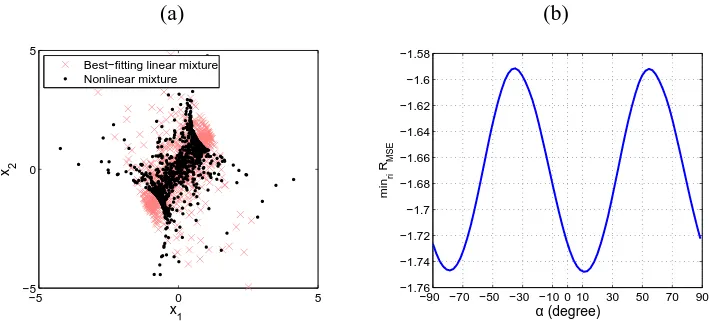
Below we give an two-channel example to illustrate the relationship between RMSE and the

orthogonal matrix U when nonlinearity in F is strong. The two independent sources are a uni-formly distributed signal and a super-Gaussian signal, and their scatter plot is given in Figure 9(a). The observations xi, whose scatter plot is shown in Figure 4(a), are generated by applying a

2-3-2 MLP to the source signals. From this figure we can see that nonlinearity in the mixing pro-cedure is comparatively strong. The orthogonal matrix U in Figure 3 is parameterized as U= [cos(α),₋sin(α); sin(α),cos(α)]. From Eq. 6 and Figure 3, one can see that RMSE depends on α

and ri. For each value of α, ri (i=1,2) are modelled by a 1-6-1 MLP and they are learned by

minimizing RMSE. Finally, minriRMSE is a function of α, with a period of 90 degrees, as plotted

in Figure 4(b). In this example,αdetermined by the MND principle is about 11 degrees. It is not that close to zero, but it is still comparatively small and consequently the sources si are recovered

approximately.

(a) (b)

−5 0 5

−5 0 5

x

1

x 2

Best−fitting linear mixture Nonlinear mixture

−90 −70 −50 −30 −10 0 10 30 50 70 90 −1.76

−1.74 −1.72 −1.7 −1.68 −1.66 −1.64 −1.62 −1.6 −1.58

α (degree)

min

ri

R

MSE

Figure 4: (a) Nonlinear mixtures of a sinusoid source signal and a super-Gaussian source signal (whose scatter plot is given in Figure 9.a) generated by a 2-3-2 MLP. x-mark points show linear mixtures of the sources which fit the nonlinear mixtures best. (b) minriRMSE as a

5. Simulations

In this section we investigate the performance of the proposed principle for solving nonlinear ICA using synthetic data. The experiments in Zhang and Chan (2007a) have empirically shown that both MND and the smoothness constraint are useful to ensure nonlinear ICA based on kernels to result in nonlinear BSS, when nonlinear distortion in the mixing procedure is not very strong. As its performance depends somewhat crucially on the choice of the kernel function, nonlinear ICA based on kernels is not used for comparison here. The following six methods (schemes) were used to separate various nonlinear mixtures:

1. MISEP: The MISEP method (Almeida, 2003) with parametersθrandomly initialized.7 Note that in this method, the smoothness constraint has been implicitly incorporated to some extent, due to the property of the adopted MLP.

2. Linear init.: The MISEP method with

G

initialized as a linear mapping. This was achieved by adopting the regularization term Eq. 2 withλ=5 (which is very large) in the first 50 epochs.

3. MND: The MISEP method incorporating MND, with RMSE, the mean square error of the best

linear reconstruction, as the regularization term (Section 2.2). The regularization parameterλ decayed fromλ0=5 toλc=0.01 in the first 350 epochs. After thatλwas fixed asλc.

4. Smooth (I): The MISEP method with the smoothness regularizer (Section 2.4) explicitly in-corporated.λdecayed from 1 to 0.004 in the first 350 epochs.

5. Smooth (II): Same as Smooth (I), butλwas fixed to 0.007.

6. VB-NICA: Bayesian variational nonlinear ICA (Lappalainen and Honkela, 2000; Valpola, 2000).8 PCA was used for initialization. After obtaining nonlinear factor analysis solutions using the package, we applied linear ICA (FastICA by Hyv¨arinen 1999 was used) to achieve nonlinear BSS.

In addition, in order to show the necessity of nonlinear ICA methods for separating nonlinear mix-tures, linear ICA (FastICA was adopted) was also used to separate the nonlinear mixtures.

It was addressed in Section 2.3 that the incorporation of direct connections between inputs and output units in the MLP representing

G

implicitly and roughly implements the MND principle. To check that, in our experiments, the MLP without direct connections and that with direct connections were both adopted to represent

G

, for comparison reasons. Like in Almeida (2003), the MLP has 20 arctan hidden units, 10 of which are connected to each of the output units of

G

.

We use the signal to noise ratio (SNR) of yi relative to si, denoted by SNR(yi), to assess the

separation performance of si. Besides, we apply a flexible nonlinear transformation h to yi to

mini-mize the MSE between h(yi)and si, and use the SNR of h(yi)relative to sias another performance

measure. In this way possible trivial transformations between siand yiare eliminated. In our

exper-iments h was implemented by a two-layer MLP with eight hidden units with the hyperbolic tangent activation function and a linear output unit. This MLP was trained using the MATLAB neural network toolbox.

7. Source code is available at http ://www.lx.it.pt/∼lbalmeida/ica/mitoolbox.html.

Three kinds of nonlinear mixtures were investigated. They are distorted source (DS) mixtures, post-nonlinear (PNL) mixtures, and generic nonlinear (GN) mixtures which are generated by a MLP. Both super-Gaussian and sub-Gaussian sources were used.

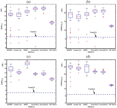
5.1 For Distorted Source Mixtures

We first considered the DS mixtures defined in Eq. 15. Specifically, in the experiments the two-channel mixtures xi were generated according to x1=a11s1+f12(s2), x2= f21(s1) +a22s2, where a11=a22=1, and f12(si) = f21(si) =3 tanh(si/4) +0.1si. We used two super-Gaussian source

signals, which are generated by si =3₅ni+2₅n3i, where ni are independent Gaussian signals. Each

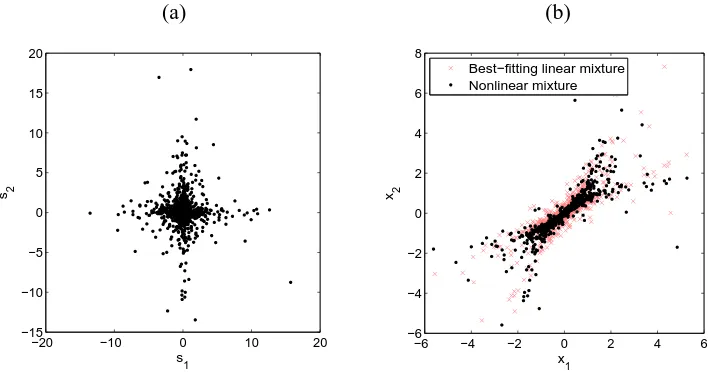
signal has 1000 samples. Figure 5 shows the scatter plot of the sources siand that of the observations xi. To see the level of nonlinear distortion in the mixing transformation, we also give the scatter plot

of the affine transformation of siwhich fits xithe best.

(a) (b)

−20 −10 0 10 20

−15 −10 −5 0 5 10 15 20

s2

s

1

−6 −4 −2 0 2 4 6

−6 −4 −2 0 2 4 6 8

x

1

x2

Best−fitting linear mixture Nonlinear mixture

Figure 5: (a) Scatter plot of the sources si generating the DS mixtures. (b) Scatter plot of the DS

mixtures xi. x-mark points are linear mixtures of siwhich fit xibest.

(a) (b)

MISEP Linear init. MND Smooth(I) Smooth(II) VB−NICA 0

2 4 6 8 10 12 14 16 18

SNR(y

1

)

Method FastICA

(dB )

MISEP Linear init. MND Smooth(I) Smooth(II) VB−NICA 0

5 10 15 20

SNR(h(y

1

))

Method FastICA

(dB )

(c) (d)

MISEP Linear init. MND Smooth(I) Smooth(II) VB−NICA 0

2 4 6 8 10 12 14 16 18 20

SNR(y

1

)

Method FastICA

(dB )

MISEP Linear init. MND Smooth(I) Smooth(II) VB−NICA 0

5 10 15 20 25 30

SNR(h(y

1

))

Method FastICA

(dB )

Figure 6: Boxplot of the SNR of separating the DS mixtures by the MLP without or with direct connections between inputs and output units. Top: Without direct connections. Bottom: With direct connections. (a, c) SNR(y1). (b, d) SNR(h(y1)).

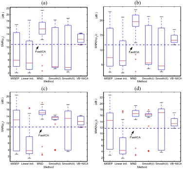
5.2 For Post-Nonlinear Mixtures

The second experiment is to separate PNL mixtures. We used two sub-Gaussian source signals, which are a uniformly distributed white signal and a sinusoid waveform. The sources were first mixed with the mixing matrix A=[-0.2261, -0.1189; -0.1706, -0.2836], producing linear mixtures z. The observations were then generated as x1=z1/2.5+tanh(3z1)and x2=z2+z32/1.5. Figure 7

shows the scatter plot of the sources and that of the PNL mixtures (after standardization). Figure 8 gives the separation performance of s1 by various methods.9 In this case, the proposed nonlinear

ICA with MND (labelled by MND) also gives almost the best results; especially for the MLP with-out direct connections, the result of nonlinear ICA with MND is clearly the best. Again, the MLP with direct connections produces better results. Moreover, one can see that compared to the DS

mixtures in Section 5.1, the PNL mixtures considered here are comparatively hard to be separated by the MLP structure.

(a) (b)

−2 −1 0 1 2

−1.5 −1 −0.5 0 0.5 1 1.5

s

1

s2

−2 −1 0 1 2

−2.5 −2 −1.5 −1 −0.5 0 0.5 1 1.5 2 2.5

x

1

x 2

Best−fitting linear mixture Nonlinear mixture

Figure 7: (a) Scatter plot of the sources si generating PNL mixtures. (b) Scatter plot of the PNL

mixtures xi.

5.3 For Generic Nonlinear Mixtures

We used a 2-2-2 MLP to generate nonlinear mixtures from sources. Hidden units have the arctan activation function. The weights between the input layer and the hidden layer are random numbers between -1 and 1. They are not large such that the mixing mapping is invertible and the nonlinear distortion produced by the MLP would not be very strong. The sources used here were the first source in Experiment 1 (super-Gaussian) and the second one in Experiment 2 (sub-Gaussian). Fig-ure 9 shows the scatter plot of the sources and that of the GN mixtFig-ures. The performance of various methods for separating such mixtures is given in Figures 10. Apparently nonlinear ICA with MND gives the best separation results in this case.

Summed over all the three cases discussed above, we can see that MISEP with MND produces promising results for the general nonlinear ICA problem, provided that nonlinearity in the mixing mapping is not very strong. Specifically, it gives the fewest unwanted solutions, and its separation performance is very good. Moreover, the MLP with direct connections usually performs better than that without direct connections, but we also found that in some cases it got stuck into unwanted solutions more easily.

5.4 On Trivial Indeterminacies

(a) (b)

MISEP Linear init. MND Smooth(I) Smooth(II) VB−NICA 2

4 6 8 10 12 14 16 18 20 22

SNR(y

1

)

Method FastICA

(dB )

MISEP Linear init. MND Smooth(I) Smooth(II) VB−NICA 5

10 15 20

SNR(h(y

1

))

Method FastICA

(dB )

(c) (d)

MISEP Linear init. MND Smooth(I) Smooth(II) VB−NICA 2

4 6 8 10 12 14 16 18 20

SNR(y

1

)

Method FastICA

(dB )

MISEP Linear init. MND Smooth(I) Smooth(II) VB−NICA 2

4 6 8 10 12 14 16 18 20 22

SNR(h(y

1

))

Method FastICA

(dB )

Figure 8: Boxplot of the SNR of separating the PNL mixtures by the MLP without or with direct connections between inputs and output units. Top: Without direct connections. Bottom: With direct connections. (a, c) SNR(y1). (b, d) SNR(h(y1)).

Figure 11 shows the relationship between yi obtained by MISEP with MND in one run and the

PC of f_∗i(si) = [f1i(si),f2i(si)]T. We can see that each yi is actually not very close to the

corre-sponding PC, which may be caused by two reasons. First, there may exist some weak non-trivial transformation in the solution, as seen from the points close to the origin in Figure 11(b); y2 is not

solely dependent on s2, but also slightly affected by s1. The other reason is the error in estimating

the density of yi or its variation involved in the MISEP method, as explained in Section 4.1.1. We

use the method proposed there to avoid the effect of the estimation error: a 1-8-1 MLP, denoted by

τi, is applied to each yi, andτi(yi)is taken as the final nonlinear ICA output. Eachτi is learned by

minimizing RMSE (Eq. 6). The resultingτi(yi)is almost identical to the corresponding PC of f∗i(si),

(a) (b)

−2 −1 0 1 2

−8 −6 −4 −2 0 2 4 6 8

s

1 s2

−5 0 5

−6 −4 −2 0 2 4 6

x

1

x2

Best−fitting linear mixture Generic nonlinear mixture

Figure 9: (a) Scatter plot of the sources si. (b) Scatter plot of the GN mixtures xi.

6. Application to Causality Discovery in the Hong Kong Stock Market

In this section we give a real-life application of nonlinear ICA with MND. Specifically, we use this method to discover linear causal relations among the daily returns of a set of stocks. The empirical results were ever reported in Zhang and Chan (2006), without much detail of the method.

6.1 Introduction

It is well known that financial assets are not independent of each other, and that there may be some relations among them. Such relations can be described in different ways. In risk management, correlations are used to describe them and help to construct portfolios. The business group, which is a collection of firms bound together in some formal and/or informal ways, focuses on ties between financial assets and has attracted a lot of interest (Khanna and Rivkin, 2006). But these descriptions cannot tell us the causal relations among the financial assets.

The return of a particular stock may be influenced by those of other stocks, for many reasons, such as the ownership relations and financial interlinkages (Khanna and Rivkin, 2006). According to the efficient market hypothesis, such influence should be reflected in the stock returns immediately. In this part we aim to discover the causal relations among selected stocks by analyzing their daily returns.10

Traditionally, causality discovery algorithms for continuous variables usually assume that the dependencies are of a linear form and that the variables are Gaussian distributed (Pearl, 2000). Under the Gaussianity assumption, only the correlation structure of variables is considered and all higher-order information is neglected. As a consequence, one obtains some possible causal

(a) (b)

MISEP Linear init. MND Smooth(I) Smooth(II) VB−NICA 0

2 4 6 8 10 12 14 16 18

SNR(y

1

)

Method FastICA

(dB )

MISEP Linear init. MND Smooth(I) Smooth(II) VB−NICA 0

2 4 6 8 10 12 14 16 18 20

SNR(h(y

1

))

Method FastICA

(dB )

(c) (d)

MISEP Linear init. MND Smooth(I) Smooth(II) VB−NICA 2

4 6 8 10 12 14 16 18

SNR(y

1

)

Method FastICA

(dB )

MISEP Linear init. MND Smooth(I) Smooth(II) VB−NICA 2

4 6 8 10 12 14 16 18

SNR(h(y

1

))

Method FastICA

(dB )

Figure 10: Boxplot of the SNR of separating the GN mixtures by the MLP without or with direct connections between inputs and output units. Top: Without direct connections. Bottom: With direct connections. (a, c) SNR(y1). (b, d) SNR(h(y1)).

grams which are equivalent in their correlation structure, and cannot find the true causal directions. Recently, it has been shown that the non-Gaussianity distribution of the variables allows us to dis-tinguish the explanatory variable from the response variable, and consequently, to identify the full causal model (Dodge and Rousson, 2001; Shimizu et al., 2006).

(a) (b)

−10 −5 0 5 10

−10 −5 0 5 10 15

Principal component of f

i1(s1)

y1

−10 −5 0 5 10

−10 −8 −6 −4 −2 0 2 4 6 8 10

Principal component of f

i2(s2)

y2

Figure 11: (a) y1recovered by MISEP with MND versus the PC of the contributions of s1to the DS

mixtures used in Section 5.1. The SNR of y1 w.r.t. the PC of the contributions of s1is

13.48dB. The dashed line is the linear function fitting the points best. (b) y2versus the

PC of the contributions of s2to the DS mixtures. The SNR is 9.12dB.

(a) (b)

−5 0 5 10

−5 0 5 10 15

Principal component of f

i1(s1) τ1

(y1

)

−10 −5 0 5 10

−10 −8 −6 −4 −2 0 2 4 6 8 10

Principal component of f

i2(s2) τ 2

(y 2

)

Figure 12: (a)τ1(y1)versus the PC of the contributions of s1to xi. τ1is modelled by a 1-8-1 MLP

and is learned by minimizing RMSE (Eq. 6). The SNR is 20.99dB. (b)τ2(y2)versus the

PC of the contributions of s2to xi. The SNR is 18.64dB.

6.2 Causality Discovery by ICA: Basic Idea

The LiNGAM model assumes that the generation procedure of the observed data follows the follow-ing properties (Shimizu et al., 2006). 1. It is recursive. This is, the observed variables xi, i=1, ...,n,

can be arranged in a causal order, such that no later variable causes any earlier variable. This causal order is denoted by k(i). 2. The value of xi is a linear function of the values assigned to the earlier

ei are independent continuous-valued variables with non-Gaussian distributions (or at most one is

Gaussian).

After centering of the variables, the causal relations among xi can be written in the matrix

form: x=Bx+e, where x= (x1, ...,xn)T, e= (e1, ...,en)T, and the matrix B can be permuted (by

simultaneous equal row and column permutations) to strict lower triangularity if one knows the causal order k(i)of xi. We then have e=Wx, where W=I−B. This is exactly the ICA separation

procedure (Hyv¨arinen et al., 2001). Therefore, the LiNGAM model can be estimated by ICA. We can permute the rows of the ICA de-mixing matrix W such that it produces a matrix fW without any zero on its diagonal (or in practice, ∑i|fWii|is maximized). Dividing each row offW by the

corresponding diagonal entry gives a new matrix fW0 with all entries on its diagonal equal to 1. Finally, by applying equal row and column permutations on B=I₋fW0, we can find the matrixBe which is as close as possible to strictly lower triangularity.B contains the causal relations of xe i. For

details, see Shimizu et al. (2006).

6.3 With Nonlinear ICA with Minimal Nonlinear Distortion

We now consider a general case of the nonlinear distortion often encountered in the data generation procedure, provided that the nonlinear distortion is smooth and mild. We use the MLP structure de-scribed in Section 3.1.1, which is a linear transformation coupled with an ordinary MLP, as shown in Figure 13, to model the nonlinear transformation from the the observed variables xito the

distur-bance variables ei.

According to Figure 13, we have e=Wx+h(x), and consequently x= (I₋W)x₋h(x) +

e, where h(x) denotes the output of the MLP. As it is difficult to analyze the relations among xi

implied by the nonlinear transformation h(x), we expect that h(x)is weak such that its effect can be neglected. The linear causal relations among xican then be discovered by analyzing W.

x _W e

MLP _h(x)

Figure 13: Structure used to model the transformation from the observed data xi to independent

disturbances ei. h(x)accounts for nonlinear distortion if necessary.

In order to do causality discovery, the separation system in Figure 13 is expected to exhibit the following properties. 1. The outputs ei are mutually independent, since independence of ei is a

crucial assumption in LiNGAM. This can be achieved since nonlinear ICA always has solutions.

2. The matrix W is sparse enough such that it can be permuted to lower triangularity. This can be

enforced by incorporating the L1 (Hyv¨arinen and Karthikesh, 2000) or smoothly clipped absolute

deviation (SCAD) penalty (Fan and Li, 2001) on the entries of W. 3. The nonlinear mapping mod-eled by the MLP is weak enough such that we just care about the linear causal relations indicated by W. To achieve that, we use MISEP with MND given in Section 3.1. In addition, we initialize the system with linear ICA results. That is, W is initialized by the linear ICA de-mixing matrix, and the initial values for weights in the MLP h(x)are very close to 0. The training process is terminated once the LiNGAM property holds for W. After the algorithm terminates, var(hi(x))

var(ei) can be used to

6.4 Simulation Study

We examined the performance of the scheme discussed in Section 6.3 for identifying linear causal relations using simulated data. To make the nonlinear distortion in the data generation procedure weak, we used the structure in Figure 13 to generate the 8-dimensional observed data xi from some

independent and non-Gaussian variables ei, that is, xi are generated by a linear transformation

cou-pled with a MLP.

The linear transformation in the data generation procedure was generated by A= (I₋B)−1_{. It}

satisfies the LiNGAM property since B was made strict lower triangular. The magnitude of non-zero entries of B is uniformly distributed between 0.05 and 0.5, and the sign is random. To examine if spurious causal relations would be caused, we also randomly selected 9 entries in the strict lower triangular part of B and set them to zero. The disturbance variables were obtained by passing independent Gaussian variables through power non-linearities with the exponent between 1.5 and 2. The variances of eiwere randomly chosen between 0.2 and 1. These settings are similar to those

in the simulation studies by Shimizu et al. (2006). The sample size is 1000. The nonlinear part is a 8-10-8 MLP with the arctan activation function in the hidden layer. The weights from the inputs to the hidden layer are between -3 and 3, that is, they are comparatively large, while those from the hidden layer to the outputs are small, such that the nonlinear distortion is weak. The nonlinear distortion level in the generation procedure is measured by the ratio of the variance of the MLP output to that of the linear output. We considered two cases where the nonlinear distortion level is 0.01 and 0.03, respectively.

We used the scheme detailed in Section 6.3 to identify the linear causal relations among xi. The

SCAD penalty was used, and there are 10 arctan hidden units connected to each output of the MLP. We repeated the simulation for 100 trials. In each trial the maximum iteration number was set to 800. The results are given in Table 1 (numbers in parentheses are corresponding standard errors). The failure rate (the chance that LiNGAM does not hold for W within 800 iterations), the percentages of correctly identified non-zero edges, correctly identified large edges (with the magnitude larger than 0.2), and spurious edges in the successful cases, and the resulting nonlinear distortion level var(hi(x))

var(ei)

in the separation system are reported. We can see that W almost always satisfies the LiNGAM property, and that most causal relations (especially large ones) are successfully identified. The settingλ=0.12, meaning that MND is explicitly incorporated, gives better results thanλ=0 does, although the difference is not large. This is not surprising because even withλ=0, nonlinear ICA with the separation structure of Figure 13 and with W initialized by linear ICA could achieve MND to some extent. However, whenλ=0.12, the nonlinear distortion in the separation system is much weaker, and we found that estimated values of the entries of B are closer to the true ones. The penalization parameter for SCAD,λSCAD, plays an important role. A largerλSCADwould make W

satisfy the LiNGAM property more easily, but as a price, in the result more causal relations tend to disappear or be weaker.

For comparison, we also used linear ICA with the de-mixing matrix penalized by SCAD11for causality discovery. The result is reported in Table 2. Even whenλSCADis very large, which causes

many causal relations to disappear, as seen from the table, there is still a high probability that the resulting de-mixing matrix fails to satisfy the LiNGAM property. These results show that for

Nonl. level inF

Settings (λ,λSCAD)

Fail. in 800 iter.

Edges iden-tified

Large edges identified

Spurious edges

Nonl. level var(hi(x))

var(ei)

0.01 (0.12,0.06) 3% 88% (11%) 99% (3%) 7% (10%) ∼0.03 (0,0.06) 3% 87% (12%) 97% (4%) 7% (9%) _∼0.06

0.03 (0.12,0.10) 1% 79% (14%) 92% (7%) 9% (11%) ∼0.08 (0,0.10) 1% 76% (12%) 89% (8%) 8% (10%) _∼0.13

Table 1: Simulation results of identifying linear causal relations among xi with the nonlinear ICA

structure Figure 13 and the SCAD penalty (100 trials). Numbers in parentheses are corre-sponding standard errors.

Nonl. level inF

Settings Fail. rate Edges iden-tified

Large edges identified

Spurious edges

0.01 λSCAD=0.2 41% 67% (13%) 79% (15%) 4% (5%)

0.03 λSCAD=0.25 54% 52% (12%) 58% (17%) 4% (7%)

Table 2: Simulation results of identifying linear causal relations among xiby linear ICA with SCAD

penalized de-mixing matrix (100 trials).

the data whose generation procedure has weak nonlinear distortion and approximately satisfies the LiNGAM property, nonlinear ICA with MND, together with the SCAD penalty, is useful to identify their linear causal relations.

6.5 Empirical Results

The Hong Kong stock market has some structural features different from the US and UK markets (Ho et al., 2004). One typical feature is the concentration of market activities and equity ownership in relatively small group of stocks, which probably makes causal relations in the Hong Kong stock market more obvious.

6.5.1 DATA

Here we aim at discovering the causality network among 14 stocks selected from the Hong Kong stock market.12 The selected 14 stocks are constituents of Hang Seng Index (HSI).13 They are almost the largest companies of the Hong Kong stock market. We used the daily dividend/split adjusted closing prices from Jan. 4, 2000 to Jun. 17, 2005, obtained from the Yahoo finance database. For the few days when the stock price is not available, we used simple linear interpolation to estimate the price. Denoting the closing price of the ith stock on day t by Pit, the corresponding

return is calculated by xit =Pit_P−_i,tP₋i,t₁−1. The observed data are xt= (x1t, ...,x14,t)T. Each return series

contains 1331 samples.

Recently ICA has been exploited as a possible way to explain the driving forces for financial returns (Back, 1997; Kiviluoto and Oja, 1998; Chan and Cha, 2001). We conjecture that nonlinear ICA would be more suitable than linear ICA to serve this task, since it seems reasonable that the

12. For saving space, they are not listed here; see the legend in Figure 15.