Data Mining and Statistical Analysis for Available Budget Allocation Pre-procurement of Manufacturing Equipment

(1)

_____________________________________________________________________________________________________

Data Mining and Statistical Analysis for Available

Budget Allocation Pre-procurement of

Manufacturing Equipment

O. O. Ojo

1*

, B. O. Akinnuli

2

and P. K. Farayibi

2

1_{Department of Mechanical Engineering, Adeleke University, P.M.B. 250, Ede, Osun State, Nigeria.}

2_{Department of Industrial and Production Engineering, Federal University of Technology, P.M.B. 704,}

Akure, Ondo State, Nigeria.

Authors’ contributions

This work was carried out in collaboration among all authors. Author OOO designed the study, performed the statistical analysis, wrote the protocol and wrote the first draft of the manuscript. Authors BOA and PKF managed the analyses of the study. Author PKF managed the literature searches. All authors read and approved the final manuscript.

Article Information

DOI: 10.9734/JERR/2019/v5i316926 Editor(s): (1) Dr. Guang Yih Sheu, Associate Professor, Chang-Jung Christian University, Taiwan. Reviewers: (1) Srinivasa Rao Kasisomayajula, Jawaharlal Nehru Technological University, India. (2)M. Bhanu Sridhar, GVP College of Engineering for Women, India. (3)Choon Sen Seah, Universiti Tun Hussein Onn, Malaysia. (4)Kholil, Sahid University Jakarta, Indonesia. Complete Peer review History:http://www.sdiarticle3.com/review-history/49157

Received 02 March 2019 Accepted 15 May 2019 Published 28 May 2019

ABSTRACT

In a situation where a decision maker faces problems of allotting the available budget on the strategic decisions in a manufacturing industry, data information plays an important role to maintain long run profit in the industry. Statistical analysis was incorporated to determine the correlational strength between the number of years and each of the strategic decisions, their confidence level, and the predicted values. This study identified the strategic areas of addressing the issues which are machine ( ), accessory ( ), spare part ( ) and miscellaneous ( ), exploring the hidden data of the selected strategic decisions from International Brewery Plc, Ilesha and statistical analysis between the number of years and each of the selected strategic decisions. The model used in this work is simple linear regression while Statistical Analysis Software “SAS” was used for its applications. After exploring the hidden data from a case study, the suggested cost of

(2)

procurement for machines, accessories, spare-parts and miscellaneous are: ₦119,975,000.00; ₦127,968,000.00; ₦134,965,000.00 and ₦33,491,500.00 respectively. From appendix, the probability of each of the strategic decision is less than 0.05 which implies that the Null-Hypothesis is rejected. The number of years has significant effect on Machines, Accessories, Spare-parts and Miscellaneous. As the number of years increases, the cost of procurement of the strategic decisions increases due to high rate of demand and consumption of their products. However, the cost of procurement may fall depending on the level of demand and maintenance culture. Besides, management of the company may ask decision maker to maintain the cost before procurement. This result may be used for further research on optimization of the available budget for equipment procurement.

Keywords: Data mining; statistical analysis; pre-procurement; budget allocation; manufacturing equipment.

1. INTRODUCTION

Allocation of limited available budget on the strategic decisions has been a major problem in industry. However, information plays an important role to maintain long run profit in the industry. Thus, data Mining (DM) and Statistics are the two disciplines which are commonly used in data analysis and knowledge extraction. Though Statistics is a traditional branch that has evolved from applied Mathematics while Data Mining is a multidisciplinary branch that has evolved from computer science, but both are used for the same purpose [1]. The growth of data mining has been massive in past decade. Its application has increased with the increase of data generation as more and more data being captured through various means of Information Technology like internet. There is a growing research in the area of databases with the help of data mining. Since data mining can be used in advance data research analysis and is capable of extracting valuable knowledge from large data sets [2].

It has emerged as a new scientific and

engineering discipline to meet such

requirements. Data Mining is commonly quoted as “solving problems by analysing data that already exists in databases”. In addition to the mining of structured and numeric data stored in data warehouses, more and more interest is now being experienced in the mining of unstructured and non-numeric data such as text and web in recent times [3].

DM is a combination of computational and statistical techniques to perform exploratory data analysis (EDA) on rather large and mostly not very well cleaned data sets (or data bases). In recent times, the issue of capturing data is not considered to be a major issue but since a huge

amount of data does not convey any information, screening of useful and non-useful data has become a major challenge. Most modern problems can electronically deal with the cumulative data from many years ago [4]. This leads to a requirement for training the data miners in statistics or statistics graduates in data mining [5].

1.1 Major Goals of Data Mining

There are different goals of data mining method for statistical analysis, but [6] identified the two types as follows:

a. Verification of user’s hypothesis

b. Discovery of new patterns that can be used for prediction and description

Data mining methods seek to discover unexpected and interesting regularities, called patterns, in presented data sets. Statistical significance testing also called as Hypothesis testing can be applied in these scenarios to select the surprising patterns that do not appear as clearly in random data. As each pattern is tested for significance, a set of statistical hypotheses are considered simultaneously. The multiple comparisons of several hypotheses simultaneously are often used in Data Mining [7].

Jure Leskovec [8] added that prediction involves using some variables or fields in the database to forecast unknown or future values of other variables of interest. Description focuses on finding human-interpretable patterns describing the data.

(3)

discovery-driven data mining. Furthermore, in the context of Data Mining, description tends to be more important than prediction. This is contrast to pattern recognition and machine learning applications where prediction is often the primary goal [9,10].

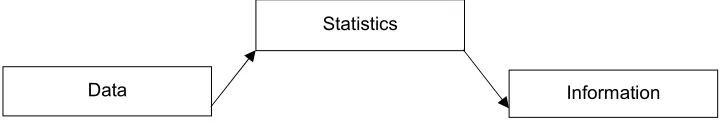
Moore [11] defined Statistics in different ways but the most suitable for this work is as illustrated below:

Data: Facts, especially numerical facts, collected together for reference or information [11]; [12].

Statistics: Knowledge communicated concerning some particular facts. Statistics is a way to get information from data. It is a tool for creating an understanding from a set of numbers [11]; [13].

1.2 Major Approaches in Statistics

A decision maker needs to be aware of the limited available resources. However, in order to minimize shortages, the past procurement records must be critically analysed to prevent

unforeseeable occurrences. Hence, the

development of the model on machines cost, accessories cost, spare parts cost and miscellaneous cost. The study would help to determine the cost of purchase of any selected strategic decisions beforehand and create a room for adjustment due to flexibility of the developed model and software. The study proposed to use Statistical Analysis Software (SAS) to analyse the extracted data of the key strategic decisions used in International Brewery Plc, Ilesha, Nigeria, and determine the level of

Fig. 1. Analysis of information through data [11]

Table 1. Major approaches for solving statistical problems

S/No. Statistics Technique Description

1 Descriptive Statistics Central Tendency

Dispersion

Shape (Graphical Display)

2 Regression

-Linear -Logistic

-Non linear -Prediction

-Modelling -Association

3 Correlation Analysis

-Pearson correlation -Spearman correlation

4 Probability Theory

-Marginal -Union -Joint

-Conditional Prediction of the behaviour of the system

defined

5 Probability Distribution

-Discrete Probability Distribution -Continuous Probability Distribution

6 Bayesian Classification Bayes’ Theorem and Naïve Bayesian

classification

7 Estimation Theory -Model Selection

-Estimating Confidence interval and significance level -ROC Curves

8 Analysis of Variance

(ANOVA)

Test equality of more than two groups mean

Data

Statistics

(4)

S/No. Statistics Technique Description

9 Factor Analysis (FA) Reduction of large no. of variables into

some general ones, also known as Data reduction Technique

10 Discriminate Analysis Predict a categorical response variable

11 Time series analysis

-Moving Average Method -Exponential smoothing -Auto regression method

Forecasting trends and seasonality

12 Quality Control Charts

-Attributes Charts -Variable charts

Display the spread of individual observation with reference to mean

13 Principal Component

Analysis

Data Reduction

14 Canonical Correlation

Analysis

15 Cluster Analysis

-Hierarchal -Non Hierarchal

16 Sampling

-Random Sampling -Non Random Sampling

Source: [14].

confidence, error terms and to predict the cost of parameters (i.e. machines cost. accessories cost, spare parts cost and miscellaneous cost) with the available budget allocation before procurement.

2. METHODOLOGY

In order to analyse the extracted data for pre-procurement of manufacturing equipment, the International Brewery Plc, Ilesha was visited to explore past procurement records. These are the following steps taken:

i. Identification of the equipment

procurement such as machines cost, accessories cost, spare parts cost and miscellaneous cost.

ii. Historical data from a case study International Brewery Plc, Ilesha, Nigeria to determine the correlational strength between the number of years and each of the strategic decisions, their confidence interval, and to predict the cost for each parameter.

iii. Modified adopted models for prediction of the cost of purchase of each strategic decision.

Determination of the hypothesis of (iii) above.

2.1 Strategic Decisions for Model Development

In this study for proper analysis, four strategic decisions were identified for pre-procurement of manufacturing equipment. They are:

a) Machine (A): A machine is a tool that consists of one or more parts, and uses energy to meet a particular goal e.g. labeller, washer, filler, pasteurizer etc. b) Accessories (B): An accessory aids the

performance of a machine e.g. beer spoon, beer paddle, beer siphon etc.

c) Spare parts (C): Spare part is an interchangeable part that is kept in an inventory and used for the repair or replacement of failed parts e.g. hose tail, cask racking spear, female equal tee etc. d) Miscellaneous (D): Other costs not

planned for but can still occur.

2.2 Statistical Analysis of the Data

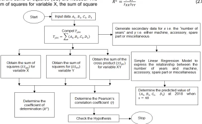
2.2.1 Simple linear regression analysis from data set

(5)

strategic decisions (i.e. machine, accessory, spare-part and miscellaneous).

Shen et al. [15] expressed the general form of a simple linear regression analysis as:

= + + (2.1)

Where:

is the predicted value for machine, accessory, spare-part and miscellaneous.

is the independent variable (i.e. number of years)

is the intercept of the regression is the slope

is error term or residual

Where:

=∑ (∑ ) (2.2)

= (∑ ) (∑ )(∑ )

(∑ ) (∑ ) (2.3)

2.2.2 Correlational strength between the number of years of procurement and the strategic decisions

Witten and Frank [16] made known that, in calculating a correlation coefficient, three different sums of squares (SS) are needed. The sum of squares for variable X, the sum of square

for variable Y and the sum of the cross-product of XY.

The sum of squares for variable X is:

= ∑( − ̅) (2.4)

Where:

is the sum of squares for variables X

̅ is the average value of X denotes data point

The sum of squares for variable Y is:

= ∑( − ) (2.5)

The sum of the cross-products ( ) is:

= ∑( − ̅)( − ) (2.6)

Therefore, Pearson’s correlation coefficient is given by:

=

( )( ) (2.7)

Shen et al. [15] added that coefficient of determination established a relationship between two variables which determines their best of fits:

= (2.8)

(6)

Table 2. Available data from international brewery, Ilesha Nigeria

Date Number of years

Machine ( )

Accessory ( )

Spare parts ( )

Miscellaneous ( )

TOTAL

1971 1 2,000,000 1,000,000 1,700,000 500,000 5,200,000

1978 8 2,500,000 1,500,000 2,000,000 600,000 6,600,000

1980 10 2,600,000 1,600,000 2,100,000 650,000 6,950,000

1981 11 2,600,000 1,600,000 2,100,000 650,000 6,950,000

1982 12 2,600,000 1,600,000 2,100,000 650,000 6,950,000

1983 13 2,600,000 1,600,000 2,100,000 650,000 6,950,000

1985 15 2,650,000 1,700,000 2,300,000 1,000,000 7,650,000

1986 16 2,650,000 1,700,000 2,300,000 1,000,000 7,650,000

1988 18 3,000,000 5,500,000 8,000,000 2,000,000 18,500,000

1989 19 3,000,000 5,500,000 8,000,000 2,000,000 18,500,000

1991 21 5,500,000 6,000,000 10,000,000 2,500,000 24,000,000

1992 22 5,500,000 6,000,000 10,000,000 2,500,000 24,000,000

1993 23 7,300,000 6,500,000 10,500,000 3,000,000 27,300,000

1994 24 32,200,000 40,000,000 45,000,000 10,000,000 127,200,000

1995 25 32,200,000 40,000,000 45,000,000 10,000,000 127,200,000

1996 26 32,200,000 40,000,000 45,000,000 10,000,000 127,200,000

1997 27 32,200,000 40,000,000 45,000,000 10,000,000 127,200,000

1998 28 32,200,000 40,000,000 45,000,000 10,000,000 127,200,000

2001 31 42,000,000 45,500,000 50,550,000 10,500,000 148,550,000

2002 32 42,000,000 45,500,000 50,550,000 10,500,000 148,550,000

2007 37 82,000,000 85,000,000 95,000,000 20,000,000 282,000,000

2008 38 82,000,000 85,000,000 95,000,000 20,000,000 282,000,000

2009 39 82,000,000 85,000,000 95,000,000 20,000,000 282,000,000

2013 43 95,000,000 96,000,000 100,000,000 25,000,000 316,000,000

2014 44 95,000,000 96,000,000 100,000,000 25,000,000 316,000,000

2017 47 120,000,000 128,000,000 135,000,000 33,500,000 416,500,000

TOTAL 845,500,000 907,800,000 1,009,300,000 232,200,000 2,994,800,000

Source: International Brewery Plc, Ilesha, 2017

2.2.3 Rule of thumb

To test the hypothesis, let the null hypothesis represents = which means that there is no significant difference and alternate hypothesis represents ≠ shows that there is significant difference between the number of years and each of the strategic decisions. If probability

≤ 0.05, “reject null hypothesis”.

The hypothesis can be tested with a t-statistic:

= (2.9)

Where:

represents the standard error of the correlation coefficient.

= (2.10)

Witten and Frank [16] stated that under null hypothesis, t-statistics has − 2 degrees of

freedom but test results are converted to before conclusions are drawn.

3. RESULTS and DISCUSSION

3.1 Application of Simple Linear Regression Model between the Number of Years and the Strategic Decisions

In order to predict or forecast the costs of procurement of machines, accessories, spare parts and miscellaneous for the year 2018, the method below suggests the amount to be spent for each of them before procuring them:

3.1.1 Predicted value for machines

Machine= + (Number of years)

Machine = 119,975,000.00

Standard Error:

(7)

= 11,171,425

95% Confidence Limits

95% C.I. = predicted ± S.E (2.064) Upper bound = 141,870,591.60 Lower bound = 98,079,408.40

To determine how well the model fits the data: variables machine and number of years:

= = 0.8589

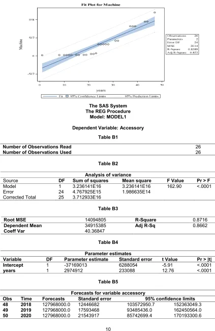
3.1.2 Predicted value for accessories

Accessories = + (Number of years)

Accessories = 127,968,000.00

Standard Error:

=

= 12,446,682

To determine how well the model fits the data: variables accessory and number of years:

= = 0.8716

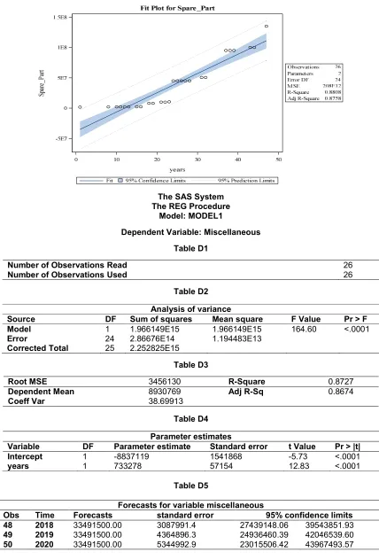
3.1.3 Predicted value for spare-parts

Spare-parts = + (Number of years) Spare-parts = 134,965,000.00

Standard Error:

=

= 13,392,197

To determine how well the model fits the data: variables spare-part and number of years:

= = 0.8808

3.1.4 Predicted value for miscellaneous

Miscellaneous = + (Number of years) Miscellaneous = 33,491,500.00

Standard Error:

=

= 3,087,991.40

To determine how well the model fits the data: variables miscellaneous and number of years:

= = 0.8727

After exploring the hidden data from a case study, the suggested cost of procurement for machines, accessories, spare-parts and

miscellaneous are: ₦119,975,000.00;

₦127,968,000.00; ₦134,965,000.00 and

₦33,491,500.00 respectively. From the appendix table A2, B2, C2 and D2, the probability of each of the strategic decision is less than 0.05 which means that the Null-Hypothesis has to be rejected. The coefficient of determination between the number of years and each of the strategic decisions has strong correlations and 95% C.I. (confidence interval) means that the amount proposed for budgeting is within the range of upper bound and lower bound which implies that the amount sets cannot exceed the upper bound but falling under the limit is good while the amount sets for lower bound cannot fall under but exceeding the limit is fine. The amount predicted is within the range of the upper and lower bound.

4. CONCLUSION AND RECOMMENDA-TION

4.1 Conclusion

The model used in this work was simple linear regression while Statistical Analysis Software “SAS” was used for its applications. Having

explored the data or past equipment

(8)

budget for equipment procurement. The number of years has significant effect on Machines, Accessories, Spare-parts and Miscellaneous. As the number of years increases, the cost of procurement of those strategic decisions increases due to high rate of demand and consumption of their products. However, the cost of procurement may fall depending on the level of demand and maintenance culture. Besides, management of the company may ask decision maker to maintain the cost before procurement, this would help the decision maker with data exploration to know exactly the amount before procurement.

4.2 Recommendation

As it is stated, data mining is the extraction of hidden information in the company. This study made use of old records for pre-procurement of the manufacturing equipment (such as machine, accessory, spare-part and miscellaneous) for available budget allocation which will subsequently be used for budgeting with the limited available budget. Therefore, this work is recommended that the procedures developed with the software “SAS” be used for budgeting, to determine the cost of procurement beforehand with the use of past procurement data and the limited available budget. This would further assist decision maker to forecast the amount to be spent on them using another tools.

COMPETING INTERESTS

Authors have declared that no competing interests exist.

REFERENCES

1. Jaya, Srivastava, Abhay, Kumar

Srivastava. Understanding linkage

between data mining and statistics. International Journal of Engineering Technology, Management and Applied Sciences (IJETMAS). 2015;3(10).

[ISSN 2349-4476]

Available:www.ijetmas.com

2. Ganesh S. Data mining: Should it be included in the statistics curriculum? The 6th international conference on teaching statistics (ICOTS 6), Cape Town, South Africa; 2002.

3. Goodman A, Kamath C, Kumar V. Data analysis in the twenty-first century. Lawrence Livermore National Laboratory (LLNL), Livermore, CA. 2008;1(1):1-3.

4. Fayyad U, Chaudhuri S, Bradley P. Data mining and its rule in database systems, Proceeding of 26th VLDB Conference. Cairo, Egypt, Morgan Kaufmanu. 2000;63– 124.

5. Stephen M. Stigler. Statistics on the table: The history of statistical concepts and methods. Cambridge, Mass: Harvard University Press; 2002.

6. Kurt Thearling. An introduction to data mining; 2010.

Available:http://www.thearling.com/text/dm white/dmwhite.htm

7. Neal Leavitt. Data mining corroborate masses; 2011.

Available:http://www.leavcom.com/ieee_m ay02.htm

Robert Nisbet et al. The handbook of statistical analysis and data mining applicants, Academic Press, ISBN: 0123747651; 2009.

Available:www.elsevierdirect.com/datamini ng

8. Jure Leskovec. Data mining: Introduction; 2010.

Available:http://www.stanford.edu/class/cs 345a/slides/01- intro.pdf

9. Gorunescu F. Data mining concepts, models and techniques. Intelligent systems reference library, Springer. 2011;12. 10. Berry MJA, Linoff GS. Mastering data

mining -The art and science of customer relationship management, New York, Wiley; 2000.

11. Moore David S. The basic practice of statistics. Third edition. W.H. Freeman and Company. New York; 2003.

12. Wiley Inter Science. Data analysis in the 21st Century; 2007.

Available:www.interscience.wiley.com 13. Stephen M. Stigler. The history of

statistics: The measurement of uncertainty before 1900, Cambridge, MA: Belknap Press of Harvard University Press; 1986. 14. Lomax RG. An introduction to statistical

concepts for education and behavioural sciences (2nd ed.). New York: Routledge; 2007.

15. Shen KS, Crossley JN, Lun WC. The nine chapters on the mathematical art. Companion and Commentary. Oxford: Oxford University Press; 1999.

(9)

Appendices

Table A

Pearson correlation coefficients, N = 26 Prob > |r| under H0: Rho=0

years Machine Accessory Spare_Part Miscellaneous

years 1.00000 0.92678

<.0001

0.93359 <.0001

0.93849 <.0001

0.93421 <.0001

Machine 0.92678

<.0001

1.00000 0.99682

<.0001

0.99450 <.0001

0.99454 <.0001

Accessory 0.93359

<.0001

0.99682 <.0001

1.00000 0.99894

<.0001

0.99681 <.0001

Spare_Part 0.93849

<.0001

0.99450 <.0001

0.99894 <.0001

1.00000 0.99366

<.0001 Miscellaneous 0.93421

<.0001

0.99454 <.0001

0.99681 <.0001

0.99366 <.0001

1.00000

The SAS System The REG Procedure

Model: MODEL1 Dependent Variable: Machine

Table A1

Number of observations read 26

Number of observations used 26

Table A2

Analysis of variance

Source DF Sum of squares Mean square F value Pr > F

Model 1 2.922218E16 2.922218E16 146.11 <.0001

Error 24 4.800132E15 2.000055E14

Corrected Total 25 3.402232E16

Table A3

Root MSE 14142330 R-Square 0.8589

Dependent Mean 32519231 Adj R-Sq 0.8530

Coeff Var 43.48913

Table A4

Parameter estimates

Variable DF Parameter estimate Standard error t Value Pr > |t|

Intercept 1 -35979715 6309256 -5.70 <.0001

years 1 2826941 233874 12.09 <.0001

Table A5

Forecasts for variable machine

Obs Time Forecasts Standard error 95% confidence limits

48 2018 119975000.0 11171425 98079408.4 141870591.6

49 2019 119975000.0 15790884 89025436.0 150924563.9

(10)

Model: MODEL1

Dependent Variable: Accessory

Table B1

Number of Observations Read 26

Number of Observations Used 26

Table B2

Source DF Sum of squares Mean square F Value Pr > F

Model 1 3.236141E16 3.236141E16 162.90 <.0001

Error 24 4.767925E15 1.986635E14

Corrected Total 25 3.712933E16

Table B3

Root MSE 14094805 R-Square 0.8716

Coeff Var 40.36847

Table B4

Intercept 1 -37169013 6288054 -5.91 <.0001

years 1 2974912 233088 12.76 <.0001

Table B5

Forecasts for variable accessory

Obs Time Forecasts Standard error 95% confidence limits

48 2018 127968000.0 12446682 103572950.7 152363049.3

49 2019 127968000.0 17593468 93485436.0 162450564.0

(11)

Model: MODEL1

Dependent Variable: Spare-part

Table C1

Table C2

Source DF Sum of squares Mean square F value Pr > F

Model 1 3.684116E16 3.684116E16 177.28 <.0001

Error 24 4.987551E15 2.078146E14

Table C3

Root MSE 14415777 R-Square 0.8808

Coeff Var 37.13566

Table C4

Intercept 1 -38092792 6431248 -5.92 <.0001

years 1 3174147 238396 13.31 <.0001

Table C5

Forecasts for variable spare_part

Obs Time Forecasts Standard error 95% Confidence limits

48 2018 134965000.0 13392197 108716775.7 161213224.3

49 2019 134965000.0 18929960 97862960.8 172067039.2

(12)

Model: MODEL1

Dependent Variable: Miscellaneous

Table D1

Table D2

Source DF Sum of squares Mean square F Value Pr > F

Model 1 1.966149E15 1.966149E15 164.60 <.0001

Error 24 2.86676E14 1.194483E13

Table D3

Root MSE 3456130 R-Square 0.8727

Coeff Var 38.69913

Table D4

Intercept 1 -8837119 1541868 -5.73 <.0001

years 1 733278 57154 12.83 <.0001

Table D5

Forecasts for variable miscellaneous

Obs Time Forecasts standard error 95% confidence limits

48 2018 33491500.00 3087991.4 27439148.06 39543851.93

49 2019 33491500.00 4364896.3 24936460.39 42046539.60

(13)

© 2019 Ojo et al.; This is an Open Access article distributed under the terms of the Creative Commons Attribution License (http://creativecommons.org/licenses/by/4.0), which permits unrestricted use, distribution, and reproduction in any medium, provided the original work is properly cited.

Peer-review history: