Bi-Level Path Following for Cross Validated Solution of Kernel Quantile Regression

(1)

Bi-Level Path Following for Cross Validated Solution of Kernel

Quantile Regression

Saharon Rosset [email protected]

Department of Statistics

The Raymond and Beverly Sackler School of Mathemetical Sciences Tel Aviv University

Tel Aviv, Israel

Editor: Ingo Steinwart

Abstract

We show how to follow the path of cross validated solutions to families of regularized optimization problems, defined by a combination of a parameterized loss function and a regularization term. A primary example is kernel quantile regression, where the parameter of the loss function is the quantile being estimated. Even though the bi-level optimization problem we encounter for every quantile is non-convex, the manner in which the optimal cross-validated solution evolves with the parameter of the loss function allows tracking of this solution. We prove this property, construct the resulting algorithm, and demonstrate it on real and artificial data. This algorithm allows us to efficiently solve the whole family of bi-level problems. We show how it can be extended to cover other modeling problems, like support vector regression, and alternative in-sample model selection approaches.1

1. Introduction

In the standard predictive modeling setting, we are given a training sample of n examples_{x1,y1}, ..., {xn,yn} drawn i.i.d from a joint distribution P(X,Y), with xi ∈Rp and yi ∈R for regression,

yi ∈ {0,1}for two-class classification. We aim to employ these data to build a model ˆY = fˆ(X)

to describe the relationship between X and Y , and later use it to predict the value of Y given new X values. This is often done by defining a family of models

F

and finding (exactly or approximately) the model f _∈

F

which minimizes an empirical loss function:∑n_i=₁L(yi,f(xi)). Examples of such

algorithms include linear and logistic regression, empirical risk minimization in classification and others.

If

F

is complex, it is often desirable to add regularization to control model complexity and overfitting. The generic regularized optimization problem can be written as:

ˆ

f=arg min

f_∈F

n

∑

i=1

L(yi,f(xi)) +λJ(f),

where J(f)is an appropriate model complexity penalty andλis the regularization parameter. Given a loss and a penalty, selection of a good value ofλis a model selection problem. Popular approaches that can be formulated as regularized optimization problems include all versions of support vector

(2)

machines, ridge regression, the Lasso and many others. For an overview of predictive modeling, regularized optimization and the algorithms mentioned above, see for example Hastie et al. (2001). In this paper we are interested in a specific setup where we have a family of regularized op-timization problems, defined by a parameterized loss function and a regularization term. A major motivating example for this setting is regularized quantile regression (Koenker, 2005). In regular-ized linear quantile regression we take the family

F

to be all linear combinations characterized by a coefficient vectorβ_∈Rp_{and the modeling problem is}

ˆ

β(τ,λ) =arg min

β n

∑

i=1

Lτ(yi−βTxi) +λkβkqq,0<τ<1,0≤λ<∞, (1)

where L_τ, the parameterized quantile loss function, has the form:

L_τ(r) =

rτ r_≥0

−r(1₋τ) r<0 ,

and is termedτ-quantile loss because its population optimizer is the appropriate quantile (Koenker,

2005):

arg min

c E(Lτ(Y−c)|X=x) =quantileτof P(Y|X=x). (2)

Because quantile loss has this optimizer, the solution of the quantile regression problems for the whole range 0<τ<1 has often been advocated as an approach to estimating the full conditional probability of P(Y_|X)(Koenker, 2005; Perlich et al., 2007). Much of the interesting information about the behavior of Y_|X may lie in the details of this conditional distribution, and if it is not nicely behaved (i.i.d Gaussian noise being the most commonly used concept of nice behavior), just

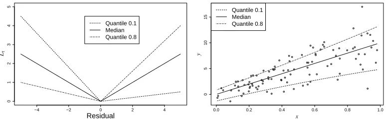
estimating a conditional mean or median is often not sufficient to properly understand and model the mechanisms generating Y . The importance of estimating a complete conditional distribution, and not just a central quantity like the conditional mean, has long been noted and addressed in various communities, like econometrics, education and finance (Koenker, 2005; Buchinsky, 1994; Eide and Showalter, 1998). There has been a surge of interest in the machine learning community in conditional quantile estimation in recent years, including theoretical analyses of consistency in quantile estimation and connections with support vector machines (Steinwart and Christmann, 2008; Christmann and Steinwart, 2008); methodological work on algorithms for quantile regression and their performance (Meinshausen, 2006; Takeuchi et al., 2006; Mease et al., 2007); and work on practical uses of extreme quantile estimation for data mining applications Perlich et al. (2007). Figure 1 shows a graphical representation of Lτ for several values ofτ, and a demonstration of the conditional quantile curves in a univariate regression setting, where the linear model is correct for the median, but the noise has a non-homoscedastic distribution.

On the penalty side, we typically use the ℓq norm of the parameters with q∈ {1,2}. Adding a

penalty can be thought of as shrinkage, complexity control or putting a prior to express our expec-tation that theβ’s should be small.

As has been noted in the literature (Rosset and Zhu, 2007; Hastie et al., 2004; Li et al., 2007; Takeuchi et al., 2009) if q_{∈ {}1,2_} and if we fix τ =τ0, we can devise path following (AKA

parametric programming) algorithms to efficiently generate the 1-dimensional curve of solutions

{βˆ(τ0,λ) : 0≤λ<∞} . Although it has not been explicitly noted by most of these authors (a

(3)

−4 −2 0 2 4

0

1

2

3

4

5

Residual

Quantile 0.1 Median Quantile 0.8

Lτ

0.0 0.2 0.4 0.6 0.8 1.0

0

5

10

15

Quantile 0.1 Median Quantile 0.8

y

x

Figure 1: Quantile loss function for some values of τ(left) and an example where the median of

Y is linear in X but the quantiles of P(Y_|X)are not because the noise is not identically distributed (right).

In addition to parameterized quantile regression, there are other modeling problems in the lit-erature which combine a parameterized loss function problem with the existence of efficient path following algorithms. These include :

1. Support vector regression (SVR, Smola and Sch¨olkopf 2004, see Gunther and Zhu 2005 for path following algorithm) withℓ1orℓ2regularization, where the parameterεdetermines the

width of the don’t care region around 0.

2. Weighted support vector machines, where the parameter of the loss function corresponds to reweighting the hinge loss differentially for the two classes, for example as a means for deriving accurate probability estimates (as recently suggested by Wang et al. 2008).

3. Huberized Lasso (Rosset and Zhu, 2007) withℓ1 regularization, where huberizing adds

ro-bustness to the traditional squared error loss, with a tunable parameter.

An important extension of theℓ2-regularized optimization problem is to non-linear fitting through

kernel embedding (Sch¨olkopf and Smola, 2002). The kernelized version of Problem (1) is

ˆ

f(τ,λ) =arg min

f

∑

_i Lτ(yi−f(xi)) +

λ 2kfk

2

HK , (3)

where_k·kHKis the norm induced by the positive-definite kernel K in the Reproducing Kernel Hilbert

Space (RKHS) it generates. The well known representer theorem (Kimeldorf and Wahba, 1971) im-plies that the solution of Problem (3) lies in a low dimensional subspace spanned by the representer functions_{K(_·,xi),i∈1, ...,n}. Following the ideas of Hastie et al. (2004) for the support vector

machine, Li et al. (2007) have shown that theλ-path of solutions to Problem (3) whenτis fixed can also be efficiently generated. A similar approach was independently developed by Takeuchi et al. (2009).

(4)

and is not part of the prediction objective (at least as long as we avoid the Bayesian view). We would therefore typically want to generate a set of modelsβ∗(τ) (or f∗(τ) in the kernel case), by selecting a good regularization parameterλ∗(τ)for every value ofτ, thus obtaining a family of good models for estimating the range of conditional quantiles, and consequently the whole conditional distribution.

This problem, of model selection to find a good regularization parameter, is often handled through cross-validation. In its simplest form, cross-validation entails having a second, indepen-dent set of data _{˜xi,y˜i}Ni=1 (often referred to as a validation set), which is used to evaluate the

performance of the models and select a good regularization parameter. For a fixedτ, we can write our model selection problem as a Bi-level programming extension of Problems (1) and (3), where

f∗(τ) =_fˆ₍_τ,λ∗₎_and_λ∗_solves

min

λ

N

∑

i=1

Lcv(y˜i,fˆ(τ,λ)T˜xi) (4)

s.t. ˆf(τ,λ)solves Problem (3) ,

where Lcv is the cross validation loss function (the bi-level formulation for Problem (1) would be identical, with ˆβ replacing ˆf ). We will assume for now that Lcv =L_τ, in order to evaluate the performance in estimating theτth quantile. The objective of this minimization problem is not convex as a function ofλ. A similar non-convex optimization problem has been tackled by Kunapuli et al. (2008) for the support vector machine, which is very similar to quantile regression from an optimization perspective (piecewise linear objective with quadratic penalty). The fundamental difference between their setting and ours is that they had a single bi-level optimization problem, while we have a family of such problems, parameterized byτ. This allows us to take advantage of internal structure to solve the bi-level problem for all values ofτsimultaneously (or more accurately,

in one run of our algorithm).

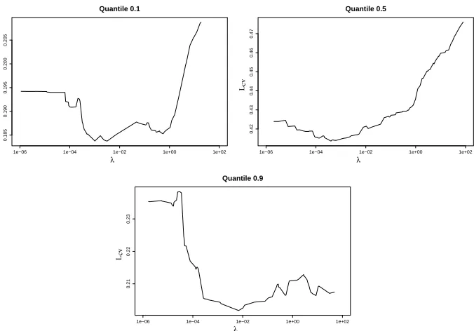
The concept of a parameterized family of bi-level regularized quantile regression problems is demonstrated in Figure 2, where we see the cross-validation curves of the objective of (4) as a function of λ for several values of τ on the same data set. As we can see, the optimal level of regularization varies with the quantile, and correct choice of the regularization parameter can have a significant effect on the success of our quantile prediction model.

(5)

1e−06 1e−04 1e−02 1e+00 1e+02

0.185

0.190

0.195

0.200

0.205

Quantile 0.1

λ Lcv

1e−06 1e−04 1e−02 1e+00 1e+02

0.42

0.43

0.44

0.45

0.46

0.47

Quantile 0.5

λ Lcv

1e−06 1e−04 1e−02 1e+00 1e+02

0.21

0.22

0.23

Quantile 0.9

λ Lcv

Figure 2: Estimated prediction error curves of Kernel Quantile Regression for some quantiles on one data set. The errors are shown as a function of the regularization parameterλ.

the properties of the modeling problems at hand, and may also benefit greatly from computational tricks and optimization shortcuts which are not the focus of this paper. We demonstrate its ability to successfully generate the complete set of cross-validated solutions on some illuminating simulation problems and on two medium-size real-life data-sets.

The rest of this paper is organized as follows. In Section 2 we discuss the properties of the quantile regression solution paths ˆf(τ,λ) and their evolution as τ changes. We then discuss in Section 3 the properties of the bi-level optimization Problem (4) and demonstrate that the solutions change predictably withτ. This is because the optimal solution always corresponds to a situation where either one of the validation points is crossing the non-differentiability elbow in the cross validation loss Lcv, or the regularization path is going thorough a knot in its piecewise linear change. However, due to the non-convexity of the problem, the solutions occasionally “jump” from one such point to another. It turns out that to follow this jumpy behavior we need to follow, not one path of solutions, but about N+n of them, corresponding to all possible candidates for Lcv optimizers.

(6)

2. Quantile Regression Solution Paths

We concentrate our discussion on the kernel quantile regression (KQR) formulation in (3), with the understanding that it subsumes the linear formulation (1) withℓ2regularization by using the linear

kernel K(x,˜x) =xT_˜x.

We briefly survey the results of Li et al. (2007) regarding the properties of ˆf(τ,_·), the optimal solution path of (3), withτfixed. Similar results were independently generated by Takeuchi et al. (2009), who concentrate on the properties of ˆf(τ,_·) with λ fixed (as we elaborate below, these problems are in fact very similar). The representer theorem (Kimeldorf and Wahba, 1971) implies that the solution can be written as

ˆ

f(τ,λ)(x) = 1

λ

"

ˆ β0+

n

∑

i=1

ˆ

θiK(x,xi) #

. (5)

For a proposed solution f(x)define:

•

E

=_{i : yi−f(xi) =0}(points on elbow of Lτ)

•

L

=_{i : yi−f(xi)<0}(left of elbow)

•

R

=_{i : yi−f(xi)>0}(right of elbow).

Then Li et al. (2007) show that the Karush-Kuhn-Tucker (KKT) conditions for optimality of a solution ˆf(τ,λ)of problem (3) can be phrased as

• i_∈

E

_{⇒ −}(1₋τ)_≤θˆi≤τ

• i_∈

L

_⇒ θˆi=−(1−τ)

• i_∈

R

_⇒ θˆi=τ

• ∑iθˆi=0.

With some additional algebra, they show that for a fixedτ, there is a series of knots, 0=λ0<λ1<

... <λm<∞such that forλ≥λmwe have ˆf(τ,λ) =constant and forλk−1<λ≤λkwe have

ˆ

f(τ,λ)(x) =1

λ λkfˆ(τ,λk)(x) + (λ−λk)hk(x)

, (6)

where hk(x) =bk₀+∑i_∈Ekb k

iK(x,xi) can be thought of as the direction in which the solution is

moving for the region λk−1<λ≤λk. The knots λk are points on the path where an observation

passes between

E

and either

L

or

R

, that is _∃i_∈

E

such that exactly θi =τ or θi =−(1−τ).

This observation may be either entering the elbow (if it was previously in

L

or

R

), or exiting it (if it previously hadθi∈(−(1−τ),τ)).2 These insights lead Li et al. (2007) to an algorithm for

incrementally generating ˆf(τ,λ) as a function of λ for fixed τ, starting from λ=∞ (where the solution only contains the interceptβ0).

2. It is clear that the definition of an observation as entering or exiting the elbow is arbitrary, since an observation which enters atλkwhen we are decreasingλactually exits atλkif we choose to traverse the path while increasingλ. There

(7)

Although Li et al. (2007) suggest it is a topic for further study, it is in fact a reasonably straight forward extension of their results to show that a similar scenario holds when we fixλ and allow τ only to change. As previously mentioned, this has been recognized and used by other authors, including Takeuchi et al. (2009) for quantile regression, and Wang et al. (2008) for weighted hinge loss. More interestingly, the same is also true when bothτ,λare changing together along a straight

line, that is, a 1-dimensional subspace of the (τ,λ) space (this has been observed by Wang et al. (2006) for SVR, which is very similar from an optimization perspective). The following lemma makes this more general result concrete. The proof relies on a study of the KKT conditions in the spirit of Li et al. (2007) and the other references above, and we omit it.

Lemma 1 Letτ(λ) =uλ+v, and denote ˆf(λ) = _f(ˆ _τ₍_λ₎_,λ_{). Then in the range}_Γ₌_{_λ_≥_{0 : 0}_< τ(λ)<1}there exist knotsλ0< ... <λmsuch that forλk−1<λ≤λk we have:

ˆ

f(λ)(x) =1

λ λkfˆ(λk)(x) + (λ−λk)hk(x)

,

where hk(x) =bk₀+∑i∈Ekb k

iK(x,xi), and the direction bk = 

 

bk₀ .. . bk_|_E

k| 



is the solution of a set of

linear equations with_|

E

_k_|+1 unknowns:

Akbk=

0

r_E

k

with

Ak=

0 1T

1 KEk

,

as defined in Li et al. (2007); and rj=yj+u· ∑i∈RkK(xj,xi)−∑i∈LkK(xj,xi)

for j_∈

E

_k.

Armed with this result, we next show the main result of this section: that the knots themselves move in a (piecewise) straight line asτchanges, and can therefore be tracked asτand the regular-ization path change. Fix a quantileτ0and assume thatλkis a knot in theλ-solution path for quantile

τ0. Further, let ikbe the observation that is passing in or out of the elbow at knotλk. Assume WLOG

that ˆθik(τ0,λk) =τ0, that is, it is on the boundary between

R

k and

E

k. Let ˜KEk be the matrix KEk

with the ikcolumn removed, and ˜bk=bkwith index ikremoved. Let si=∑j_∈R_∪L_∪{ik}K(xi,xj)for

i_∈

E

_k. Let sEk be the vector of all these values.

Theorem 2 Any knotλk moves linearly asτchanges. That is, there exists a constant ck such that

for quantileτ0+δthere is a knot in theλ-solution path atλk+ckδ, forδ∈[−εk,νk], a non-empty

neighborhood of 0. ckis determined through the solution of another set of|

E

k|+1 linear equations

with_|

E

_k_|+1 unknowns

Bk

˜bk

ck

=

−(_|

R

_|+_|

L

_|+1) −sEk

,

with

Bk=

0 1T

0

1 K˜Ek −yEk

(8)

And the fit at this knot progresses as

ˆ

f(τ0+δ,λk+ckδ) =

1 λk+ckδ

λkfˆ(λk,τ0)(x) +δhk(x)

(7)

hk(x) =˜bk0+

∑

i∈Ek−ik

˜bk

iK(x,xi) +

∑

i∈L_∪R_∪{ik}

K(x,xi). (8)

Proof For smallδ, the modified knot should be characterized byθik=τ0+δ, and

L

,

R

,

E

remaining

the same. If we can find a ck such that this holds for quantileτ0+δ andλ=λk+ckδ, and also

the KKT conditions are maintained, we have our knot for quantile τ0+δ. Assume this can be

accomplished by moving in a direction hk as in Equations (7) and (8). For the KKT conditions to

hold we need to maintain:

C1. ˆf(τ0+δ,λk+ckδ)(xi) =yi, ∀i∈

E

C2. ˆθi(τ0+δ,λk+ckδ) =θˆi(τ0,λk) +δ, ∀i∈

L

∪

R

∪ {ik}

C3. ∑_i_∈Ek−{ik}˜b k

i =−|

L

∪

R

∪ {ik}|

where C1 maintains the observations in

E

at the elbow, C2 maintains the equality requirements on ˆ

θfor the observations in

L

_∪

R

(and the one on the boundary), and C3 maintains the constraint that the ˆθ’s sum to 0.

We can express C1 in terms of Equations (7) and (8) and condition C2:

ˆ

f(τ0+δ,λk+ckδ)(xi) =yi, ∀i∈

E

⇔ hk(xi) =˜bk0+

∑

j∈Ek−ik

˜bk

jK(xj,xi) +

∑

j_∈L_∪R_∪{ik}

K(xj,xi) =ckyi, ∀i∈

E

, (9)

where the last term on the RHS of (9) accounts for the changes in the ˆθj which C2 implies for

j_∈

L

_∪

R

_{∪ {}ik}.

Now, by combining C3 and (9) into one set of equations in matrix notation, we get the result of the theorem:

˜bk

ck

=Bk

−1 −(|

R

|+|

L

|+1)

−sEk

and moving in the direction of the solution of this matrix equation as in (7,8) maintains the KKT conditions and the observation at the elbow, hence is a knot on theλ-solution path for quantileτ+δ

for every (small enough)δ.

This theorem tells us that we can in fact track the knots in the solution efficiently asτchanges. We still have to account for various types of events that can change the direction the knot is moving in. The valueθifor a point in

E

k− {ik}can reachτor−(1−τ), or a point in

L

∪

R

may reach the

elbow

E

. These events correspond to knots crossings, that is, the knotλk is encountering another

knot (which is tracking the other event). There are also knot birth events, and knots merge events, which are possible but rare, and somewhat counter-intuitive. We defer the details of how these are identified and handled to the detailed algorithm description (Appendix A). When any of these events occurs, the set of knots has to be updated and their directions have to be re-calculated using Lemma 1, Theorem 2 and the new identity of the sets

E

,

L

,

R

and the observation ik. This in essence allows

(9)

3. The Bi-level Optimization Problem

Our next task is to show how our ability to track the knots asτchanges allows us to track the solution of the bi-level optimization Problem (4) asτchanges. The key to this step is the following result.

Theorem 3 When the cross validation loss is the quantile loss (i.e., LCV=L_τ), then any minimizer3 of (4) is always either at a knot in theλ-path for thisτor a point where a validation observation crosses the elbow. In other words, one of the two following statements must hold:

• λ∗is a knot:_∃i_{∈ {}1...n_}s.t. ˆf(τ,λ∗(τ))(xi) =yi andθi∈ {τ,−(1−τ)}, or

• λ∗_{is a validation crossing:}_∃_i_{∈ {}_1..._N_}_{s.t. ˆ}_f₍_τ,_λ∗₍_τ₎₎₍_˜x_i_{) =}_y_˜_i

Proof Define ˜

L

,

R

˜ in the obvious way, as the sets of validation observations with negative and positive residuals, respectively, for a given model. Fixτ, and consider the cross validation loss for a given value ofλ:

Lcv(λ) :=

N

∑

i=1

Lcv(y˜i,fˆ(λ)(˜xi)) =

∑

i∈L˜

(1₋τ)(f(ˆ λ)(˜xi)−y˜i) +

∑

i∈R˜

τ·(y˜i−fˆ(λ)(˜xi)) =

= τ

∑

i∈R˜

yi−(1−τ)

∑

i∈L˜

yi−τ

∑

i∈R˜

ˆ

f(λk)(˜xi) + (1−τ)

∑

i∈L˜

ˆ

f(λk)(˜xi) +

+(λ−λk)

λ



−τ

∑

i∈R˜

(hk(˜xi)−fˆ(λk)(˜xi)) + (1−τ)

∑

i∈L˜

(hk(˜xi)−fˆ(λk)(˜xi)) 



where k is such thatλk₋1≤λ≤λk (where the list ofλ.’s now combines both knots and validation

crossings), and we take advantage of the representation in (6). From the last two rows we can see that Lcv is monotone inλas long as ˜

L

,

R

˜ are fixed (i.e., no validation crossing occurs) and hk is

fixed (i.e., no knot is encountered). Therefore any local (or global) extremum must be at a knot or a validation crossing.

Corollary 4 Given the complete solution path forτ=τ0, the solutions of the bi-level Problem (4) for a range of quantiles around τ0 can be obtained by following the paths of the knots and the validation crossings only, asτchanges.

To implement this corollary in practice, we have two main issues to resolve:

1. How do we follow the paths of the validation crossings?

2. How do we determine which one of the knots and validation crossings is going to be optimal for every value ofτ?

The first question is easy to answer when we consider the similarity between the knot following problem we solve in Theorem 2 and the validation crossing following problem. In each case we

(10)

have a set of elbow observations whose fit must remain fixed asτchanges, but whose ˆθvalues may vary; sets

L

,

R

whose ˆθare changing in a pre-determined manner withτ, but whose fit may vary freely; and one special observation which characterizes the knot or validation crossing. The only difference is that in a knot this is a border observation from the training set, so both its fit and its

ˆ

θare pre-determined, while in the case of validation crossing it is a validation observation, whose fit must remain fixed (at the elbow), but which does not even have a ˆθvalue. Taking all of this into account, it is easy to show the following result, closely related to Theorem 2. Assume there is a validation crossing atλv for quantileτ0, and that validation set observation jv is the one crossing

the elbow, that is,

ˆ

f(τ0,λv)(˜xjv) =0.

Let sEv,KEv,bEv be defined as in Theorem 2 (with {iv}=Φ for definition of s). Let kv =

(K(XEv,˜xjv))be a 1×|

E

v|vector of the kernel evaluations at ˜xjvfor the elbow observation

function-als.

Proposition 5 λv moves linearly as τ changes. That is, there exists a constant dv such that for

quantileτ0+δthere is a validation crossing in the λ-solution path at λv+dvδ, forδ∈[−εv,νv],

a non-empty neighborhood of 0. dv is determined through the solution of a set of |

E

v|+2 linear

equations with_|

E

_v_|+2 unknowns:

Bv _˜b_v dv =  

−(_|

R

_|+_|

L

_|) −sEv

−s˜jv





with

Bv=





0 1T ₀

1 KEv −yEv

1 kv −y˜jv 

.

Furthermore, the solution ˆf(τ0+δ,λv+cvδ)is given by:

ˆ

f(τ0+δ,λv+cvδ) =

1 λv+cvδ

λvfˆ(λv,τ0)(x) +δhv(x)

hv(x) =˜bv0+

∑

i∈Ev

bv_iK(x,xi) +

∑

i_∈L_∪R

K(x,xi).

The proof relies on following the same steps as the proof of Theorem 2 and is omitted for brevity. The second question we have posed requires us to explicitly express the validation loss (i.e.,

Lτ on the validation set) at every knot and validation crossing in terms of δ, so we can compare them and identify the optimum at every value ofδ. Using the representation in (7) we can write the

validation loss for a knot k (denote fk(δ) =_fˆ₍_τ₀₊_δ,λ_k₊_c_k_δ₎_): ∑N

i=1 Lcv(y˜i,fk(δ)(˜xi)) =

=₋(1−τ0−δ)

∑

i∈L˜

(y˜i−fk(δ)(˜xi)) + (τ0+δ)

∑

i∈R˜

(y˜i−fk(δ)(˜xi)) =

=

N

∑

i=1

Lcv(y˜i,fk(0)(˜xi)) +δ

∑

i

|y˜i−fk(0)(˜xi)|+_λ δ k+ckδ·

(10)

·



−(1−τ0−δ)

∑

i∈L˜

(ckfk(0)(˜xi)−hk(˜xi)) + (τ0+δ)

∑

i∈R˜

(ckfk(0)(˜xi)−hk(˜xi)) 

(11)

A similar expression can be derived for validation crossings (with fk,ck,hk replaced by fv,dv,hv

in the obvious way). These are rational functions ofδwith quadratic expressions in the numerator and linear expressions in the denominator. Our cross-validation task can be re-formulated as the identification of the minimum of these rational functions among all knots and validation crossings, for every value ofτin the current segment, where the directions hk,hv of all knots and validation

crossings are fixed (and therefore so are the coefficients in the rational functions). This is a

lower-envelope tracking problem, which has been extensively studied in the literature (Sharir and Agarwal

1995 and references therein). The algorithms developed mostly conform to the common-sense ap-proach of maintaining the order of the validation loss scores from smallest to largest; identifying the τvalues where elements with neighboring scores meet (i.e., obtain identical score); and whenever a meeting occurs, re-calculating only the relevant crossing points, that is, those of the elements that changed order and their immediate neighbors. We also have to re-calculate some of the validation loss scores whenever an event happens on the training solution path (like a knot crossing).

To calculate the meeting point of two elements with neighboring scores (assume WLOG that they are two knots k,l) we find the zeros of the cubic equation obtained by requiring equality for the

two rational functions of the form (10) corresponding to the two elements. Writing the expression in (10) for both k and l, and requiring equality gives us the cubic equation:

0= λkλl(lok−lol) + (11)

+δ[(λkcl+λlck)(lok−lol) +λkλl(lak−lal) +λl(τ0LRk−Lek)−λk(τ0LRl−Lel)]

+δ2[ckcl(lok−lol) + (ckλl+clλk)(lak−lal) +

+cl(τ0LRk−Lek) +λlLRk−ck(τ0LRl−Lel)−λkLRl]

+δ3_[c

kcl(lak−lal) +clLRk−ckLRl],

where:

lok= N

∑

i=1

Lcv(y˜i,fk(0)(˜xi))

lak=

∑

i

|y˜i−fk(0)(˜xi)|

LRk=

∑

i∈L˜

(ckfk(0)(˜xi)−hk(˜xi)) +

∑

i∈R˜

(ckfk(0)(˜xi)−hk(˜xi))

Lek=

∑

i∈L˜

(ckfk(0)(˜xi)−hk(˜xi)),

with similar expressions for the elements with subscript l derived in the obvious way. The smallest non-negative solution forδis the one we are interested in.

(12)

0.30 0.31 0.32 0.33 0.34 0.35 0.36 0.37

10

11

12

13

Knot crossing

knot 1 − train knot 1 − CV knot 2 − train knot 2 − CV valid. crossing − CV

τ Lτ

Figure 3: Illustration of the process of lower envelope tracking, in the presence of two knots and one validation crossing being tracked. See text for details.

that the linearity of the solid and dashed lines in Figure 3 is for illustration simplicity, and is not a realistic depiction of the non-linear evolution of the loss asτvaries, as discussed above.

4. Algorithm Overview

Bringing together all the elements from the previous sections, we now give a succinct overview of the resulting algorithm (Algorithm 1). Since there is a multitude of details, we defer a detailed pseudo-code description of our algorithm to Appendix A.

The algorithm follows the knots of theλ-solution path asτchanges using the results of Section 2, and keeps track of the cross-validated solution using the results of Section 3. Every time an

event happens (like a knot crossing), the direction in which two of the knots are moving has to be

changed, or knots have to be added or deleted. Between these events, the evolution of the cross-validation objective at all knots and cross-validation crossings has to be sorted and followed. Their order is maintained and updated whenever crossings occur between them.

4.1 Approximate Computational Complexity

Looking at Algorithm 1, we should consider the number of steps of the two loops and the complexity of the operations inside the loops. Even for a “standard”λ-path following problem for fixedτ, it is in fact impossible to rigorously bound the number of steps in the general case, but it has been argued and empirically demonstrated by several authors that the number of knots in the path behaves as

O(n), the number of samples (Rosset and Zhu, 2007; Hastie et al., 2004; Li et al., 2007). In our case the outer loop of Algorithm 1 implements a 2-dimensional path following problem, that can be thought of as following O(n)1-dimensional paths traversed by the knots of the path. It therefore stands to reason (and we confirm it empirically below) that the outer loop typically has O(n2₎

(13)

Algorithm 1: Main steps of our algorithm

Input: The entireλ-solution path for quantileτ0; the bi-level optimizerλ∗(τ0) Output: Cross-validated solutions f∗(τ)forτ_∈[τ0,τend]

Initialization: Identify all knots and validation crossings in the solution path forτ0; Find

1

direction of each knot according to Theorem 2 ;

Find direction of each validation crossing according to Proposition 5; 2

Create a list M of knots and validation crossings sorted by their validation loss ; 3

Letλ∗(τ0)be the one at the bottom of the list M, and f∗(τ0)accordingly ; 4

Calculate future meeting of each pair of neighbors in M by solving the cubic equation 5

implied by (10); Setτnow=τ0;

6

whileτnow<τenddo

7

Find valueτ1>τnowwhere first knot crossing occurs;

8

Find valueτ2>τnowwhere first knot merge occurs;

9

Find valueτ3>τnowwhere first knot birth occurs;

10

Setτnew=min(τ1,τ2,τ3);

11

whileτnow<τnewdo

12

Find valueτ4>τnowwhere first future meeting (order change) in M occurs;

13

Find valueτ5>τnowwhere first validation crossing birth occurs;

14

Find valueτ6>τnowwhere first validation crossing cancelation occurs;

15

Setτnext=min(τ4,τ5,τ6,τnew);

16

Updateλ∗(τ),f∗(τ)forτ∈(τnow,τnext)as the evolution of the knot or validation

17

crossing attaining the minimal Lcvin M (i.e., the one atλ∗(τnow)) ;

Update M according to the first event (order change, birth, cancelation); 18

Update the future meetings of the affected elements using (10); 19

Setτnow=τnext;

20

end

21

Update the list of knots according to the first event (knot crossing, birth, merge) ; 22

Update the directions of affected knots using Theorem 2 ; 23

end

24

of the algorithm (i.e., many iterations of the outer loop may have no events happening in the inner loop). Each iteration of either loop requires a re-calculation of up to three directions (of knots or validation crossings), using Theorem 2 or Proposition 5. These calculations involve updating and inverting matrices that are roughly_|

E

_{| × |}

E

_|in size (where _|

E

_|is the number of observations in the elbow). However note that only one row and column are involved in the updating, leading to a complexity of O(n+_|

E

_|2₎_{for the whole direction calculation operation, using the}

Sherman-Morrison formula (Sherman and Sherman-Morrison, 1949) for updating the inverse. In principle,_|

E

_|can be equal to n, although it is typically much smaller for most of the steps of the algorithm, on the order of√n or less. So we assume here that the loop cost is between O(n)and O(n2₎_.

(14)

falls well short of a formal “worst case” complexity calculation, but we offer it as an intuitive guide to support our experiments below and get an idea of the dependence of running time on the amount of data used.

We have not considered the complexity of the lower envelope tracking problem in our analysis, because it is expected to have a much lower complexity (number of order changes

O(max(n,N)log(max(n,N)))and each order change involves O(1)work).

5. Extensions

In this section we discuss some of the possible extensions of our algorithm. First we discuss the design of algorithms that are similar in spirit for other parameterized loss function problems, in particular for support vector regression (ε-SVR) and Huberized least squares regression. We then move on to the use of in-sample model selection criteria instead of cross validation. Finally, we address the issue of possible non-monotonicity in τ, noted by previous authors (Koenker, 2005; Takeuchi et al., 2006). We demonstrate how our algorithm can be naturally extended to amend this situation.

5.1 Support Vector Regression and Weighted Support Vector Machines

One possible view of regularized ε-SVR (Smola and Sch¨olkopf, 2004) is similar to the quantile regression problem forτ=0.5:

ˆ

f(ε,λ) =arg min

f

∑

_i Lε(yi−f(xi)) +

λ 2kfk

2

HK (12)

where the parameterized loss function Lε is piecewise linear and symmetric around zero, with a

don’t care region of size 2ε:

L_ε(r) =







r₋ε r_≥ε

0 ₋ε<r<ε

−r₋ε r_{≤ −}ε

.

The loss is parameterized byε. From an optimization perspective, this problem is very similar to KQR, with a piecewise linear loss and an RKHS norm penalty. The solution can be represented as in (5), and the KKT conditions for optimality of solutions of (12) in terms of coefficients of representer functions have been formalized and used to designλ-path following algorithms by Gunther and Zhu (2005). For example, if we define for a proposed solution f(x)ofε-SVR:

•

L

=_{i : yi−f(xi)<−ε}(points on left of left elbow of Lε)

•

E

L={i : yi−f(xi) =−ε}(left elbow)

•

C

=_{i :_|yi−f(xi)|<ε}(don’t care region)

•

E

R ={i : yi−f(xi) =ε}(right elbow)

•

R

=_{i : yi−f(xi)>0}(right of right elbow),

(15)

• i∈

C

_⇒ _θˆ_i₌₀

• i∈

L

_⇒ _θˆ_i₌₋₁

• i∈

R

_⇒ _θˆ_i₌₁

• i_∈

E

L ⇒ −1≤θˆi≤0

• i_∈

E

R ⇒ 0≤θˆi≤1

• ∑iθˆi=0.

Wang et al. (2006) have noted thatε-paths (with fixedλ) can similarly be followed. Because of the fundamental similarity in the optimization setting, all our results regarding behavior ofλ-paths and knots asτchanges in quantile regression (e.g., Theorem 2) can be adapted in a reasonably straight forward manner to follow paths and knots ofλ-solution paths inε-SVR, asεvaries.

There is, however, a fundamental difference in the statistical setting between parameterized quantile loss and parameterizedε-SVR loss. While every quantile loss function defines an interest-ing modelinterest-ing problem of estimation of a given conditional quantile, there is no such clear motivation for varyingε. Furthermore, there is no obvious way in which the cross validation loss should change withε, if at all. In most cases, it seemsεis viewed more as another tuning parameter for a single modeling problem (likeλ), than a parameter defining a range of loss functions, each of its own in-dependent interest. In this situation, the only motivation for solving the range of bi-level problems parameterized byεmay be as a way to efficiently traverse the entire(ε,λ)solution space in search of a single “best” prediction model. It may therefore be appropriate to use a single cross validation objective Lcvindependent ofε. If we choose Lcv=Lτ=0.5(the symmetric quantile loss, sometimes

called absolute loss), then our observations on the bi-level path following problem (e.g., Theorem 3) would require slight modifications, but the ideas would carry through to theε-SVR case in a straight forward manner.

An interesting recent development is the proposal of weighted support vector machines for probability estimation by Wang et al. (2008). Their proposed approach calls for fitting weighted versions of the support vector machine, with a range of relative weights applied to the two classes, as a provably valuable approach for estimating probabilities. We omit the details for brevity, but note that like the SVR case above, extending our bi-level approach to this problem is straight forward.

5.2 ℓ1-regularized Huberized Squared Loss

Rosset and Zhu (2007) suggested the use of robust versions of squared error loss withℓ1

regular-ization, as an approach for combining computational efficiency and robustness to long-tailed error distribution. Huber’s loss function is quadratic for small absolute residuals, then continues linearly as the residuals move away from zero, while maintaining differentiability. It is parameterized with a huberizing point t:

Lt(r) =

r2 _|r_|<t

2t_|r_{| −}r2 otherwise .

The algorithm proposed in Rosset and Zhu (2007) for λ-path following can be thought of as an extension of the LARS-Lasso algorithm proposed for the Lasso (squared error loss withℓ1penalty)

(16)

there are still knots), the KKT conditions are quite different, and if we also use a differentiable Lcv,

the cross validation procedure would be affect as well. However, the general reasoning of this paper can still be applied to build bi-level path following algorithms for the Huberized lasso problem, and to choose good t,λcombinations.

5.3 Use of In-sample Model Selection Criteria

Li et al. (2007) follow the literature in proposing two model selection criteria for selectingλ∗ for a fixed value ofτ, when there is no validation sample. These are Schwartz information criterion (SIC, Schwarz, 1978) and generalized approximate cross validation (GACV, Yuan, 2006). Both of these use the model’s effective degrees of freedom (DF) as a complexity measure which penalizes the empirical error. Following Zou et al. (2007), Li et al. (2007) show that an unbiased estimate of DF is the size of the elbow_|

E

_|. Thus, they arrive at following SIC and GACV approximations:

SIC(λ) = log 1

n

∑

i=1

Lτ(yi−fˆ(τ,λ)(xi)) !

+log n

2n |

E

| (13)

GACV(λ) = ∑

n

i=1Lτ(yi−fˆ(τ,λ)(xi))

n_{− |}

E

_| . (14)

If we were to adopt these measures (or similar ones) for model selection instead of the cross validation approach using an independent validation set, tracking the optimal solutionλ∗(τ)requires no extra work besides following the knots of the solution (as described in Sections 2, 4). This is guaranteed by the following simple result:

Proposition 6 For any fixedτ, the minimizerλ∗(τ)of SIC, GACV and any similar model selection criterion which is monotone in both∑n_i=₁Lτ(yi−fˆ(τ,λ)(xi))and|

E

|, is always at one of the knots

of the solution path.

Proof The loss is monotone between knots (e.g., from looking at Equation 6), while_|

E

_|is fixed.

Thus, if we wish to use SIC or similar measures for selectingλ∗(τ), the inner loop of Algorithm 1 (lines 12-21) can be omitted and replaced with a simple tracking of the value of SIC at the knots that are being followed. Since the algorithmic complexity of applying SIC/GACV is reduced com-pared to cross validation, and given the ongoing debates in the literature on the merits of in-sample versus out-of-sample model selection, it may often be beneficial to apply these in-sample methods in addition, or even instead of, cross validation. We demonstrate and compare performance of the two approaches in Section 6 below.

5.4 Addressing Quantile Crossings

The problem of quantile crossing, as formulated by Koenker (2005), is that for any fixed λ (in particularλ=0 in the linear quantile regression case, which is the one that Koenker (2005) concen-trates on), the prediction ˆf(τ,λ)(x)may not be non-decreasing inτfor a fixed x. That is, we may haveτ0<τ1and ˆf(τ0,λ)(x)>fˆ(τ1,λ)(x), which can never be true of the corresponding population

conditional quantiles, of course.

(17)

in our case, since our algorithm is local in nature and generates the solutions for the complete space of(τ,λ)values. However, we can offer a partial remedy to the quantile crossing problem through observation of the guaranteed sub-optimality of the resulting solutions, and a consequent envelope

tracking modification. The main motivation is the following:

Proposition 7 Assumeτ0<τ1and ˆf(τ0,λ)(x)>fˆ(τ1,λ)(x)for someλ,x. Then either

EY|X=xLτ0(Y,fˆ(τ0,λ)(x))≥EY|X=xLτ0(Y,fˆ(τ1,λ)(x)). (15) or

EY|X=xLτ1(Y,fˆ(τ0,λ)(x))≤EY|X=xLτ1(Y,f(ˆ τ1,λ)(x)) (16) Thus, we can always improve the predictive quality of either ˆf(τ0,λ)or ˆf(τ1,λ)by eliminating the non-monotonicity.

Proof In what follows we eliminate the explicit conditioning in the expectations. All expectations

are with regard to the distribution P(Y_|X =x). Denote by c0 and c1 the τ0 andτ1 quantiles

re-spectively of P(Y_|X=x). By definition, c0≤c1. We also assume ˆf(τ0,λ)(x)> fˆ(τ1,λ)(x). We

hereafter denote these two fitted value by ˆf0,f1ˆ respectively for brevity. This gives us three possible scenarios:

1. ˆf1≥c0. In this case (15) holds, since:

EL_τ0(Y,fˆ0) = τ0

Z

y≥_fˆ₀y−

ˆ

f0dP(y|x) + (1−τ0)

Z

y<_fˆ₀−y+

ˆ

f0dP(y|x) = τ0

Z

y≥_fˆ₀P(Y ≥y|x)dy+ (1−τ0)

Z

y<_fˆ₀P(Y ≤y|x)dy = ELτ0(Y,f1) +ˆ

Z fˆ₀

ˆ

f1

[(1₋τ0)P(Y _≤y_|x)₋τ0P(Y _≥y_|x)]dy ≥ ELτ0(Y,f1)ˆ ,

where the inequality on the last line is because P(Y_≤y_|X=x)_≥τ0in the range ˆf1≤y≤fˆ0

(by our assumption that c0≤f1ˆ < f0ˆ).

2. ˆf0≤c1. By the same line of argument in this case (16) holds.

3. If neither of the previous two holds, we must have ˆf1<c0_≤c1< f0ˆ. Following the same steps as in case 1 we write:

ELτ0(Y,f0) =ˆ ELτ0(Y,f1) +ˆ

Z fˆ₀

ˆ

f1

[(1₋τ0)P(Y_≤y_|x)₋τ0P(Y _≥y_|x)]dy (17)

ELτ1(Y,f0ˆ) = _ELτ1(Y,f1ˆ) +

Z fˆ₀

ˆ

f1

[(1−τ1)P(Y≤y|x)−τ1P(Y ≥y|x)]dy. (18)

AssumeEL_τ0(Y,_fˆ₀₎_<_E_L_τ0_(Y_,_fˆ₁₎_{. It implies the integral in (17) is negative which in turn} implies that the integral in (18) is also negative, since trivially

∂ ∂τ

Z fˆ0

ˆ

f1

[(1₋τ)P(Y_≤y_|x)₋τP(Y _≥y_|x)]dy<0.

(18)

The following is an immediate consequence of Proposition 7 if we take P(Y_|˜xi)to be a point mass

at Y =y˜i.

Corollary 8 If non-monotonicity holds at a validation point, that is, τ0<τ1 and ˆf(τ0,λ)(˜xi)>

ˆ

f(τ1,λ)(˜xi), then either

Lτ0(y˜i,fˆ(τ0,λ)(˜xi))≥Lτ0(y˜i,fˆ(τ1,λ)(˜xi))

or

L_τ1(y˜i,fˆ(τ0,λ)(˜xi))≤Lτ1(y˜i,fˆ(τ1,λ)(˜xi)).

Thus, we can improve our holdout performance at either quantileτ0orτ1by appropriately enforcing monotonicity.

We conclude that eliminating non-monotonicity can improve both predictive performance and cross validation performance. In terms of practical implications, it is easy to see (though not trivial to implement) how our algorithm can be extended to identify quantile crossings. When these occur, at least one knot will be moving in the ‘wrong direction’, that is, the expression in (7) will be decreasing inδ. The algorithm will then have to keep careful tabs on the upper and lower limits of the fit at every λ as τ changes (the quantile-crossing gap). Discussion of the details and the appropriate way to resolve the non-monotonicity given this envelope is left for future work.

6. Experiments

Our methodology offers a new approach for generating the full set of cross-validated kernel quantile regression models. There are several interesting aspects of the modeling problem in general and our algorithm in particular that should be studied through a data-based study.

First, to evaluate the new algorithm, the efficiency of the algorithm should be compared to alternative approaches that allow generation of complete set of solutions and cross-validation. This includes the naive grid-based search whereby the KQR problem is solved using standard approaches (Takeuchi et al., 2006) for a grid of values in the(τ,λ)space, and a good regularization parameter is chosen for each value ofτby cross-validation; and the method of Li et al. (2007), which can be used to generate the completeλ-path at a grid ofτ-values and cross validate each path separately. As Li et al. (2007) demonstrated clearly, theirλ-path method is far superior to the grid-based approach in terms of computation, and so we concentrate on comparison to theλ-path approach only, and show that our algorithm compares favorably to it in generating the full set of bi-level solutions.

Second, we may also be interested in studying properties of the modeling problem, not necessar-ily tied to the new algorithm. Cross-validation based selection of regularization should be compared to in-sample approaches such as SIC (Schwarz, 1978) and GACV (Yuan, 2006). As noted above, all of these can be implemented in our framework. It is obvious that given the same amount of data for model fitting, it is better to use holdout data for model selection. However, the fair comparison should be between integrating the validation set into the training set and implementing an in-sample model selection approach, and using a smaller training set in a cross-validation framework.

Another interesting question about the modeling approach regards the ability of KQR to deal with skewed and non-homogeneous error distributions, and still generate reasonable estimates of the underlying quantiles.

(19)

0.0 0.2 0.4 0.6 0.8 1.0

−1

0

1

2

3

4

y

x

0.2 0.4 0.6 0.8

5e−04

5e−03

5e−02

5e−01

τ ˆλ(τ

)

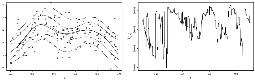
Figure 4: Left: The function f(x)(solid), data points drawn from it with i.i.d normal error, and our cross-validated estimates of quantiles 0.1,0.25,0.5,0.75,0.9 (dashed lines, from bottom to top). Right: Evolution of optimal regularization parameter ˆλ(τ), asτvaries.

6.1 Simulations

Our simulation setup starts with univariate data x_∈[0,1]and a “generating” function f(x) =2_· exp(₋30_·(x₋0.25)2_{) +}_sin₍π_·_x2₎

(see Figure 4). We then let Y = f(x) +ε, where the errorsε

are independent, with a distribution that can be either:

1. ε_∼N(0,1), that is, i.i.d standard normal errors

2. ε+ (x+1)2_∼_exp₍_1/_(x₊₁₎2₎_{, which gives us errors that are still independent and have mean}

0, but are asymmetric and have non-constant variance, with small signal-to-noise ratio on the higher values of x (see Figure 5).

Figure 4 demonstrates the results of the algorithm with i.i.d normal errors, 200 training samples and 200 validation samples and a Gaussian kernel with parameterσ=0.2. In the left panel, we see that the quantile estimates all capture the general shape of the true curve, with some “smoothing” due to regularization. In the right panel we see the evolution of the optimal regularization parameter ˆ

λ(τ)asτvaries. We see the expected “jumpy” behavior of the optimal parameter, but we do not see a clear tendency to be smaller for quantiles closer to 1/2. This is somewhat surprising when we think in terms of bias and variance (or approximation error and estimation error) in learning. Values ofτ closer to 1/2 typically create learning problems that are “easier”, that is, variance is smaller (Koenker, 2005), and this should in principle allow us to build more complex models (reduce regularization), and decrease bias. A confounding factor in this analysis is the fact that the scale of quantile error need not be comparable for different quantiles. In particular, we may expect that loss magnitude would be larger for quantiles close to 0.5, where both types of errors get penalized equally. If that is the case, then having the similar regularization parameter may in fact imply less regularization forτclose to 0.5 compared to extreme quantiles. Another interesting observation is that whileλ∗(τ)may be jumpy, both the empirical and the validation loss may vary smoothly. This smoothness is in fact guaranteed for the validation loss Lcv, since it is easily seen that the “jumps”

are points where validation loss is equal at two knots or validation crossings.

(20)

NTRAIN NSTEPS TIME(BI-LEVEL) TIME(LI ET AL.) BREAK-EVEN RESOLUTION

200 29238 931SEC. 2500SEC. 3000

100 12269 99SEC. 900SEC. 900

50 2249 23SEC. 480SEC. 400

Table 1: Number of steps and run times of our algorithm and of Li et al. (2007), for the whole path fromτ=0.1 toτ=0.9, as a function of the number of training observations NTRAIN. These results are based on applying Li et al. (2007) at 8000 different values ofτ. The last column shows what resolution would give similar running times to both approaches (see text for details).

of Li et al. (2007), who have already demonstrated that their algorithm is significantly more effi-cient than grid-based approaches for generating 1-dimensional paths for fixedτ. Table 1 shows the number of steps of the main (outer) loop of Algorithm 1 and the total run time of our algorithm for generating the complete set of cross-validated solutions forτ_∈[0.1,0.9]as a function of the num-ber of training samples (with validation sample fixed at 200). Also shown is the run time for the algorithm of Li et al. (2007), when we use it on a grid of 8000 evenly spacedτvalues in[0.1,0.9]

and find the best cross validated solution by enumerating the candidates as identified in Section 3. Our conjecture that the number of knots in the 2-dimensional path behaves like O(n2₎_{seems to be}

consistent with these results, as is the hypothesized overall time complexity dependence of O(n3₎_.

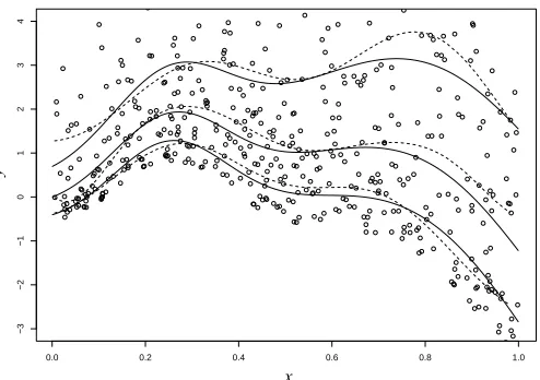
Since 8000 is typically an unnecessarily fine grid for practical applications, we offer in the last column an evaluation of the comparative efficiency of the two methods in terms of the number of distinctτ values that can be fitted with the Li et al. (2007) approach in roughly the same running time as our approach. It is clear from these results that if just a small number ofτvalues (say, 10) are sufficient to address the complete problem, our approach does not carry a computational benefit. Next, we demonstrate the ability of KQR to capture the quantiles with “strange” errors from model 2. Figure 5 shows a data sample generated from this model and the(0.25,0.5,0.75)quantiles of the conditional distribution P(Y_|X) (solid), compared to their cross-validated KQR estimates (dashed), using 500 samples for learning and 200 for validation (more data is needed for learning because of the very large variance at values of x close to 1). As expected, we can see that estimation of the lower quantiles, and at smaller values of x is easier, because the distribution P(Y_|X =x)has long right tails everywhere and has much larger variance when x is big.

6.2 Baseball Data and California Housing

As discussed in Perlich et al. (2007), estimating conditional quantiles is often a modeling task that is well grounded in practical applications. In the context of house prices, we can think of estimat-ing a high (but not extreme4) conditional quantile as the seller’s search for a favorable bargaining position in negotiations. Similarly for salaries, estimating a high conditional quantile can serve as a measure of what an employee can expect to receive optimistically (but still realistically), given his characteristics and performance.We therefore demonstrate KQR on two well studied data sets that correspond to such modeling problems: baseball salaries as a function of a player’s home runs and years of experience (He et al., 1998) and the California housing data set (Pace and Barry, 1997),

(21)

0.0 0.2 0.4 0.6 0.8 1.0

−3

−2

−1

0

1

2

3

4

y

x

Figure 5: Quantiles of P(Y_|X)(solid), and their estimates (dashed) for quantiles (0.25,0.5,0.75)

with the exponential error model.

which describes the median prices of houses in neighborhoods of California along with nine ex-planatory demographic variables. We seek to demonstrate predictive performance, fitted models and the relative performance of different model selection approaches.

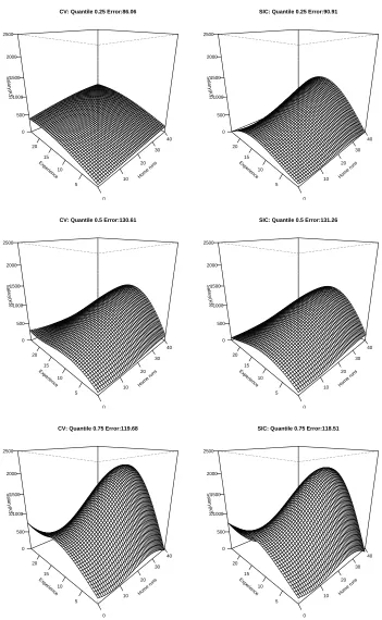
For our experiments, we use a Gaussian kernel, with the parameter γ=1 chosen based on experimentation, to give flexible but not overly jumpy fits. We demonstrate the fit and accuracy of model selection using CV compared to using SIC. For CV, we used 50 of the 263 players in the data set for validation (selection of ˆλ(τ)) and 50 more for testing the accuracy of the resulting model. Thus, 163 examples were used for training. For SIC, we used 213 (training+validation) as the training set, and applied Equation (13) for selecting ˆλ(τ). Both approaches were evaluated using the 50 test observations. In Figure 6 we show the resulting fit in both approaches, for three different quantiles. As expected, compensation seems to be monotone in performance (home runs) but not in experience (salary tends to increase as players gain experience, but then decreases as they get older and performance deteriorates). As we can see, the model-selected surfaces are quite similar between CV and SIC, though this need not be the case, as we should keep in mind that SIC is choosing between models trained on more data. In terms of accuracy on the test set (shown above each plot), The results are also very comparable. When comparing the two approaches we should also keep in mind the reduced complexity of applying SIC, and the existing literature on instability of CV-based model selection, though this is not evident in our results.

(22)

Home runs 0 10 20 30 40 Experience 5 10 15 20 Salary(K$) 0 500 1000 1500 2000 2500

CV: Quantile 0.25 Error:86.06

SIC: Quantile 0.25 Error:90.91

(23)

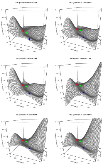
On each plot the fit at San Francisco (red circle), Los Angeles (blue square) and Sacramento (green triangle) are marked. We can see that the selected fits using CV and SIC are quite similar, with possible exception to the more jumpy fit selected by SIC for quantile 0.5. The valid insights that seem to arise out of these plots relate to the lower house values in the central valley of California compared to the coastal area, and the reduced house values in the Sacramento area compared to near by the Bay Area.

7. Conclusions and Future Work

In this paper we have demonstrated that the family of bi-level optimization Problems (4) defined by the family of loss functions L_τ can be solved via a path following approach which essentially maps the whole surface of solutions ˆf(τ,λ) as a function of bothτ andλ and uses insights about the possible locations of the bi-level optima to efficiently find them. This leads to a closed-form algorithm for finding f∗(τ)for all quantiles. We see two main contributions in this work: a. Char-acterization of a family of non-convex optimization problems of great practical interest which can be solved using solely convex optimization techniques and b. Formulation of a practical algorithm for generating the full set of cross-validated solutions for the family of kernel quantile regression problems.

We have shown how our approach can be extended to other modeling problems with a parame-terized loss function, such as SVR, and to other versions of KQR, including using in-sample model selection criteria and enforcing monotonicity on the resulting quantiles.

There are many other interesting aspects of our work, which we have not touched on here, including: development of further optimization shortcuts to improve algorithmic efficiency, inves-tigation of the range of applicability of our algorithmic approach beyond KQR and SVR, analysis of the use of various kernels for KQR and how the kernel parameters and kernel properties interact with the solutions, and more extensive empirical studies.

It is of particular interest to us to investigate the bias-variance tradeoff in loss function selection. As we have mentioned, modeling with the quantile loss function Lτ leads to estimation of theτth quantile of P(Y_|x)in the decision theoretic sense that the population optimizer of the loss function is this quantile (see Equation 2). However, this by no means guarantees that a model learned from finite data using Lτ (with or without regularization) will do well in predicting the τth quantile. In particular, there is no guarantee that a model built using a different loss function (say, L_η,η₆=τ)

will not do better in predicting this quantile. This can be thought of in terms of bias and variance, where the model generating quantileηis similar enough to the one for quantileτ(i.e., bias is small), but it is “easier” to learn with L_η, that is, variance is smaller, which would typically be the case if ηis closer to 1/2 than τ(Koenker, 2005). A detailed investigation of this question is outside the scope of the current work, but will be a natural extension.

A particularly important and difficult type of quantile estimation problems pertains to estimation of extreme quantiles (e.g., τ=0.01 orτ=0.99) which can serve as approximations for expected extreme values of the function being estimated. These problems are typically very difficult

statis-tically, that is, hard because of the scarcity of information implicit in trying to estimate events we

(24)

Latitude (N) 34 36 38 40 Longitude (W) 116 118 120 122 124

Median house price(K$)

10 12 14 16 18 20