Effect of Local Density Dependence on the Exchange and Direct Part of A-A Interaction Potential

(1)

INTRODUCTION

The most famous models used for deriving the interaction potential are the two–center shell

model1-3_{, the energy density formalism}4-7_{, the}

proximity method8_{and the double folding model}9_.

Recently, the double folding model was developed in two ways .The first is the calculation of its exchange part using finite range NN force. This development produces some computational difficulties if the non diagonal densities, appearing in this part, were not approximated using the density

matrix expansion method of Negele and Vautherin10_.

The other development is the use of realistic effective NN force which is usually density

dependent11-16_{. Again density dependence of NN}

force produces difficulties in numerical calculations. To overcome this difficulty the nucleon–nucleon separation distance in the density dependent NN force is considered when calculating the direct HI potential part and is neglected for the exchange part. This approximation in considering the density dependence of NN interaction needs to be tested.

The Generalized Double Folding Model

The double-folding model17-18_{proved to be}

quite successful in obtaining the correct values of the real part of the optical model potential needed

Effect of local density dependence on the

exchange and direct part of

αα

α

-

α

αα

interaction potential

**M.Y. ISMAIL, H. ELGEBALY* and M.M. OSMAN**

Physics Department, Faculty of Science, Cairo University, Cairo (Egypt).

(Received: May 09, 2010; Accepted: June 21, 2010)

ABSTRACT

The study show that the error in neglecting s-dependence affects strongly both the values of U_ex and U_tot . This effect is about 30 %( 23%) in U_ex (U_tot) for the force BDM3Y₂-Reid type while it is less than 7% for BDM3Y₁-Ried. It decreases as α– α separation distance increases. For BDM3Y₃ type force the corresponding error is too large at separation distance R=0.

Key words: α−α interaction potential, local density dependence.

to fit elastic scattering data. In this model the real

potential U_n(R) is the sum of the direct part U_D(R)

and the exchange part U_ex(R). Earlier studies led to

the calculation of the real potential on the assumption that the exchange part of the

nucleon-nucleon interaction is a zero range19-20_{. Such}

approximation produces correct ion-ion potential in the tail region only.

The inner and surface regions can not be

calculated with good accuracy using δ -force

assumption. However, it is well established now that in certain cases of nuclear scattering observed

first in α-particle21_{and later for other light HI}

systems22-24_{, where the data are sensitive to the HI}

optical potential over a wider radial domain, the

simple double folding model17-18_{failed to give a good}

description to the data. Therefore, some further developments of the folding model have been made to obtain a more realistic shape of the folding potential. One of these approaches is to impose on

the widely used M3Y-NN interaction25_{explicit density}

dependence, the DDM3Y1 interaction26_{. Another is}

to treat correctly the simple Knock out effect arising from the Pauli principle. In the later approach the exchange part of the real HI optical potential is derived from the first principle instead of using a

(2)

calculation with M3Y and DDM3Y1 interactions 5,26,32_.

In ref. 11-16,33_{a simple microscopic approach has}

been developed based on generalization of the

double folding and the density matrix34-35_{. In the}

framework of this model, the real part of the HI optical potential at a separation distance R between the centers of two ions is obtained by:

...(1)

where i and j refer to the

single-particle wave functions of nucleons in the two

colliding nuclei A₁ and A₂, respectively_; V_D and V_Ex

are the direct and exchange parts of the effective NN interaction.

In this work we calculate the full ion-ion

potential, U_n(R) =U_D(R)+U_ex(R) , for α–α nuclear

pairs in the frame wor k of the generalized

double folding model14,25_{using the effective}

BDM3Y14-16,25,36-37_{nucleon-nucleon force. This work}

is show the accuracy of neglecting the S-dependence in the density-dependent NN interaction on both the direct and exchange parts

of α–α interaction potential.

Calculation of The Exchange And Direct HI Potential Using Density Dependent NN Forces

In general, the exchange part of the real

heavy ion potential must be non-local35_{. Since the}

exact treatment of the non-local exchange term is too complicated and needs a lot of numerical calculations, one usually obtains the equivalent local potential by representing the relative-motion wave function of the two interacting nucleons as plane

wave35_{. Under such an assumption, the exchange}

part of the HI potential11-18_{is represented by,}

...(2)

By introducing the one –body density

matrix11-16_{, one can explicitly write equation (2) as:}

...(3)

where kr(R) is the relative –motion

momentum given by [11-16]

...(4)

where M and E_c.m are the reduced mass,

and relative energy in the center of

mass system and m is the nucleon mass. Here U_n(R)

and V_c(R) are total nuclear potential (U_n(R) = U_D(R)+

U_ex(R)), and coulomb potential, respectively. For

density dependent NN force equitation (3) can be written as,

...(5)

where

) s , R ( Gex r r

is given by [ 12,38]

...(6)

where density matrix expansion was used to simplify the non-diagonal density of the target nucleus. In most calculations [11-16] the s-dependence in the function F is neglected. In this case the direct and exchange parts of HI potential are not computed in consistent way regarding to the variables of density dependence in NN force. The function F has the following expression for BDM3Yn (n=1,2,3) type of forces

...(7)

β have the values =1,2 and 3. The projectile

non-diagonal density matrix can be expanded using

DME39_{or it can be calculated exactly using oscillator}

model if the projectile is double closed shell light

nucleus (as O16_{and He}4 _{)[34]. If one neglects the}

s-dependence in ρ appearing in the function F, it

becomes

(3)

In general

ex G depends on both the

magnitude and direction of

ex U ( )R

. In this case, it is very difficult to calculate . So, we should use approximate methods to take into account the s-dependence in density dependent part of NN force. We use the approximations [40-42 respectively],

...(9)

, ...(10)

and

...(11)

Taking

Rr

in Z-direction and integrating

over the variable

y

φ

, to get,

...(12)

where

ex G (R,s)

is given by [16,38]

...(13)

where . Since the nucleon

relative momentum depends on the total real potential (equation (5)), the calculation of Uex need UD as input.

The direct part of α-α potential is given

by,

...(14)

where

This shape of density dependence is used

usually in the calculation of the direct part of the HI

-potential, where the ρ-dependence of the NN

potential is evaluated at the two positions of the interacting nucleons. This procedure is not consisting with that used in calculating the exchange part of the potential. For this part the density in the NN exchange force is evaluated at the mid point separating the two nucleons. This means

T

p

ρ

+

in the NN force is taken as:

...(15)

The aim of the present part is to estimate the effect of the difference between the two

approaches on the direct α-α potential42_.The

method of calculating the direct part using NN force depends on the density given by equation (14) is well known. It depends on taking the Fourier transform of the NN potential which depends on s. This reduces the six-dimensional integral of HI direct potential to integration over one-dimensional integrals. On the other hand equation (15) for the density dependence produces difficulties in calculating, the direct part of HI potential .In this case,

...(16)

This can be simplified by changing the integration variables to

r and r insted r and

s 1 2

r r r r

to get,

...(17)

Equation (17) can be calculated when one assumes similar target and projectile nuclei with Gaussian shapes for densities. Taking Gaussian forms for the density distributions of both target and projectile

...(18)

(4)

Substituting equations (18) and (19) into equation (17) and using the spherical harmonics basis then integrating over the solid angle of

r of angle -and

s r

r

_ϕ

For similar projectile and target nuclei

( ), the last expression is

simplified to

...(20)

Where

This expression can be easily calculated numerically.

RESULTS AND DISCUSSION For exchange part

Since the exact treatment of s-dependence in calculating nucleus-nucleus is too difficult. We use the approximations in equations

(9-11). For α-particle,

...(21)

where

b 1 α=

and b is the oscillator parameter and it has the value b= (1.33) fm.

The effect of taking s-dependence in density appearing in NN force is to produce more

attractive α-α interaction potential at small

separation distances. The tables show that the error in neglicting s-dependence affects strongly both the

values of U_ex and U_tot .

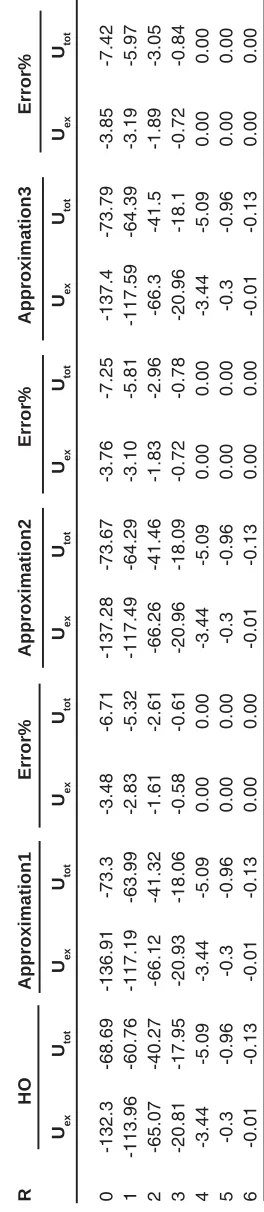
Table (1) contains the results for the

separation distance variation of the α-α interacting

pair calculated using BDM3Yn (n=1,2,3)- Reid force. Table (2) is the same as Table (1) expect Paris version of NN force was used. Part (a), (b) and (c) denote calculations using BDM3Yn with n=1,2 and 3 respectively. Both the tables were calculated for

projectile energy per nucleon E_L/A_P= 5.2 MeV/N.

The first column of each table shows the value of the nucleus-nucleus separation distance (R), the

second column shows both Uex and U_D+Uex (

denoted by U_tot) . The second column was calculated

using harmonic oscillator wave function to construct the diagonal and non diagonal densities. The third, forth and fiftieth column are our calculations by using the three approximations. The error on the tables are calculated as

Tables (1) and (2) show the results of α-α

calculated using a value b=1.33. The tables show that the effect of neglecting s-dependence increases as the NN force becomes corresponding to higher value of incompressibility coefficient. This effect is

about 30%(23%) in U_ex (U_tot) for the force BDM3Y₂

-Reid type while it is less than 7% for BDM3Y₁-Ried.

It decreases as the α–α separation distance

increases. For BDM3Y₃ type of force which

corresponds to large value of compressibility coefficient, the corresponding error is too large at separation distance R=0, as Tables (1c) and (2c) indicate .This error becomes reasonable as the

separation distance between the two α particles

increases. The huge error obtained is due to the

small radius of α–particle (about 1.58 fm.) and its

large central density. Since the force BDM3Y₃

corresponds to nuclear matter saturation curve in

which

A E

varies strongly when ρ becomes greater

than the saturation density ρ( 0.17fm3)

0

−

≅ ,we expect

large change in potential when the density changes

slightly .In other words the force BDM3Y₃ is too

sensitive to the value of ρ when the latter has value

more than 0.17 fm-3_{. In order to decrease this}

error, á –particle is artifficially made less localised. For this purpose we increased

r 2

1 2

by about 13% to becomes (1.83 fm.) which corresponds to b=1.5 fm. Tables (3a) and (3b) are the same as (1c) and (2c) respectively except they are calculated using

b=1.5fm. These tables show that when the α–

particle becomes less localised, the error becomes reasonable.

For direct part

(5)

T

able 1a: Calculation of the exchange and tot

al

ααααα

-

α α α α α

potential using density dependent (BDM3Y

1

-Reid) NN interaction. Harmonic oscillator

wave functions used in the calculations to construct the densities. The second column covers r and s to calculations using

⎟ ⎠ ⎞ ⎜ ⎝ ⎛ − +⎟ ⎠ ⎞ ⎜ ⎝ ⎛ + = s s r r r r 2 1 r ρ 2 1 r ρ ρ 2 P 1 T

which the other columns are calculated by approximating the expression

()

(

)

₂ P 1 T r ρ r ρ ρ r r + = .b=1.33 fm. R H O Approximation1 Error% Approximation2 Error% Approximation3 Error% Uex Utot Uex Utot Uex Utot Uex Utot Uex Utot Uex Utot Uex Utot 0 33.06 -22.79 -12.85 -68.7 138.87 -201.45 -16.01 -71.86 148.43 -215.31 -17.3 -73.15 152.33 -220.97 1 -14.48 -30.84 -34.84 -51.2 -140.61 -66.02 -36.78 -53.14 -154.01 -72.31 -37.52 -53.88 -159.12 -74.71 2 -31.38 -29.39 -34.35 -32.37 -9.46 -10.14 -34.76 -32.77 -10.77 -11.50 -34.88 -32.89 -11.15 -11.91 3 -11.38 -15.84 -11.58 -16.04 -1.76 -1.26 -11.62 -16.07 -2.11 -1.45 -11.63 -16.08 -2.20 -1.52 4 -1.81 -4.6 -1.82 -4.61 -0.55 -0.22 -1.82 -4.61 -0.55 -0.22 -1.82 -4.61 -0.55 -0.22 5 -0.15 -0.82 -0.15 -0.82 0.00 0.00 -0.15 -0.82 0.00 0.00 -0.15 -0.82 0.00 0.00 6 -0.01 -0.1 -0.01 -0.1 0.00 0.00 -0.01 -0.1 0.00 0.00 -0.01 -0.1 0.00 0.00 T

able 1(b): Is the same as T

able (1a) but using density dependent ( BDM3Y

(6)

T

able 2(a): Is the same as T

able (1a) but for M3Y

Paris R H O Approximation1 Error% Approximation2 Error% Approximation3 Error% Uex Utot Uex Utot Uex Utot Uex Utot Uex Utot Uex Utot Uex Utot 0 -132.3 -68.69 -136.91 -73.3 -3.48 -6.71 -137.28 -73.67 -3.76 -7.25 -137.4 -73.79 -3.85 -7.42 1 -113.96 -60.76 -117.19 -63.99 -2.83 -5.32 -117.49 -64.29 -3.10 -5.81 -117.59 -64.39 -3.19 -5.97 2 -65.07 -40.27 -66.12 -41.32 -1.61 -2.61 -66.26 -41.46 -1.83 -2.96 -66.3 -41.5 -1.89 -3.05 3 -20.81 -17.95 -20.93 -18.06 -0.58 -0.61 -20.96 -18.09 -0.72 -0.78 -20.96 -18.1 -0.72 -0.84 4 -3.44 -5.09 -3.44 -5.09 0.00 0.00 -3.44 -5.09 0.00 0.00 -3.44 -5.09 0.00 0.00 5 -0.3 -0.96 -0.3 -0.96 0.00 0.00 -0.3 -0.96 0.00 0.00 -0.3 -0.96 0.00 0.00 6 -0.01 -0.13 -0.01 -0.13 0.00 0.00 -0.01 -0.13 0.00 0.00 -0.01 -0.13 0.00 0.00 T

able 1(c): Is the same as T

(7)

T

2 ) force R H O Approximation1 Error% Approximation2 Error% Approximation3 Error% Uex Utot Uex Utot Uex Utot Uex Utot Uex Utot Uex Utot Uex Utot 0 -57.25 -50.4 -71.13 -64.29 -24.24 -27.56 -72.22 -65.37 -26.15 -29.70 -72.7 -65.85 -26.99 -30.65 1 -75.19 -47.7 -83.22 -55.73 -10.68 -16.83 -83.93 -56.45 -11.62 -18.34 -84.22 -56.74 -12.01 -18.95 2 -60.17 -35.05 -61.93 -36.81 -2.93 -5.02 -62.14 -37.02 -3.27 -5.62 -62.21 -37.09 -3.39 -5.82 3 -20.29 -16.66 -20.44 -16.81 -0.74 -0.90 -20.47 -16.84 -0.89 -1.08 -20.47 -16.84 -0.89 -1.08 4 -3.21 -4.82 -3.22 -4.82 -0.31 0.00 -3.22 -4.82 -0.31 0.00 -3.22 -4.82 -0.31 0.00 5 -0.26 -0.9 -0.26 -0.9 0.00 0.00 -0.26 -0.9 0.00 0.00 -0.26 -0.9 0.00 0.00 6 -0.01 -0.12 -0.01 -0.12 0.00 0.00 -0.01 -0.12 0.00 0.00 -0.01 -0.12 0.00 0.00 T

able 2(c): Is the same as T

able (2a) but using density dependent (BDM3Y

(8)

T

able 3(a): Is the same as T

a

ble (1c) but for using b=1.5 fm

R H O Approximation1 Error% Approximation2 Error% Approximation3 Error% Uex Utot Uex Utot Uex Utot Uex Utot Uex Utot Uex Utot Uex Utot 0 -53.17 -62.33 -59.2 -68.36 -11.34 -9.67 -59.68 -68.83 -12.24 -10.43 -59.88 -69.04 -12.62 -10.77 1 -51.27 -56.51 -55.07 -60.31 -7.41 -6.72 -55.4 -60.63 -8.06 -7.29 -55.53 -60.77 -8.31 -7.54 2 -36.09 -40.81 -37.09 -41.81 -2.77 -2.45 -37.19 -41.91 -3.05 -2.70 -37.23 -41.95 -3.16 -2.79 3 -15.05 -20.84 -15.17 -20.96 -0.80 -0.58 -15.19 -20.98 -0.93 -0.67 -15.2 -20.98 -1.00 -0.67 4 -3.6 -6.88 -3.61 -6.89 -0.28 -0.15 -3.61 -6.89 -0.28 -0.15 -3.61 -6.89 -0.28 -0.15 5 -0.51 -1.53 -0.51 -1.53 0.00 0.00 -0.51 -1.53 0.00 0.00 -0.51 -1.53 0.00 0.00 6 -0.04 -0.25 -0.04 -0.25 0.00 0.00 -0.04 -0.25 0.00 0.00 -0.04 -0.25 0.00 0.00 T

able (2c) but for using b=1.5 fm

(9)

Table 4(a): Results of the direct part of a-a potential for BDM3Y₁-Reid NN force using oscillator model densities with b=1.33 fm for the density of a particle. V_s(R) is calculated using

⎟ ⎠ ⎞ ⎜ ⎝ ⎛ + ⎟ ⎠ ⎞ ⎜ ⎝ ⎛ +

= s

2 1 -r ρ s 2 1 r ρ

ρ _p r₁ r _T r₂ r

and V(R) calculated using ρ ρp

( )

r1 ρT

( )

r2 r r ₊

=

t = 4 fm-1 _{t=2.5 fm}-1 _{Full range}

R V( R) V_s(R) Error V( R) V_s(R) Error V( R) V_s(R) Error

0 386.17 375.7 -2.79 -384.3 -364.3 -5.48 1.87 11.37 83.52

1 318.42 314.03 -1.4 -318.8 -309.8 -2.9 -0.35 4.24 108.32

2 169.06 170.82 1.03 -174.7 -178 1.84 -5.68 -7.19 21.06

3 53.03 54.41 2.54 -59.57 -62.91 5.31 -6.54 -8.5 23.06

4 9.47 9.75 2.87 -12.51 -13.46 7.01 -3.04 -3.7 17.91

5 0.97 1 2.74 -1.7 -1.85 7.83 -0.73 -0.85 13.86

6 0.06 0.07 15.83 -0.17 -0.21 21.36 -0.11 -0.14 24.19

Table 4(b): Is the same as Table (4a) but using density dependent BDM3Y₂ force

0 241.05 215.09 -12.07 -256 -208.6 -22.73 -14.95 6.51 329.69

1 237.37 229.01 -3.65 -242.8 -225.9 -7.49 -5.48 3.09 277.22

2 155.09 159.07 2.5 -158.3 -165.8 4.53 -3.17 -6.7 52.69

3 51.51 53.13 3.05 -57.26 -61.43 6.79 -5.75 -8.3 30.75

4 9.01 9.19 2.05 -11.94 -12.68 5.89 -2.93 -3.49 16.02

5 0.9 0.91 1.36 -1.59 -1.68 4.94 -0.7 -0.77 9.17

6 0.05 0.06 15.59 -0.15 -0.19 19.04 -0.1 -0.13 20.81

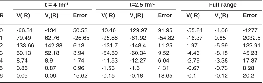
Table 4(c): Is the same as Table (4a) but using density dependent BDM3Y₃ force

0 -66.31 -134 50.53 10.46 129.97 91.95 -55.84 -4.06 -1277

1 79.49 62.76 -26.65 -95.86 -61.92 -54.82 -16.37 0.85 2032.5

2 133.66 142.38 6.13 -131.7 -148.4 11.25 1.97 -5.99 132.91

3 50.13 52.18 3.94 -54.59 -60.34 9.52 -4.46 -8.15 45.28

4 8.74 8.9 1.74 -11.53 -12.27 6.04 -2.79 -3.38 17.37

5 0.86 0.87 0.96 -1.53 -1.6 4.31 -0.67 -0.73 8.28

6 0.05 0.06 15.62 -0.15 -0.18 18.65 -0.1 -0.12 20.2

dependence on the HI potential we consider

α

-α

interacting potential. The small mass number of

α

-particle produces large changes in the density distribution along the separation distance between the two centers of the interacting particles. This change in the density from point to point makes the

(10)

Table 5(a): Is the same as Table (4a) but for M3Y Paris

0 465.36 448.28 -3.81 -401.7 -373.8 -7.49 63.61 74.53 14.65

1 393.3 386.15 -1.85 -340.1 -327.5 -3.84 53.2 58.63 9.27

2 218.96 221.83 1.3 -194.2 -198.8 2.31 24.8 23.08 -7.45

3 71.39 73.64 3.06 -68.52 -73.21 6.4 2.87 0.43 -561.6

4 13.06 13.52 3.39 -14.71 -16.03 8.26 -1.65 -2.51 34.42

5 1.36 1.41 3.15 -2.03 -2.23 9.08 -0.67 -0.82 19.18

6 0.09 0.1 15.72 -0.2 -0.26 22.04 -0.11 -0.16 26.15

Table 5(b): Is the same as Table (4b) but using density dependent BDM3Y₂ force

0 228.74 186.41 -22.71 -221.9 -155.4 -42.77 6.85 30.99 77.91

1 261.16 247.52 -5.51 -233.7 -209.9 -11.3 27.49 37.58 26.87

2 196.19 202.68 3.2 -171.1 -181.6 5.8 25.12 21.09 -19.14

3 68.91 71.55 3.69 -65.28 -71.13 8.23 3.63 0.42 -762

4 12.3 12.61 2.44 -13.9 -14.95 7.01 -1.6 -2.35 31.59

5 1.23 1.25 1.57 -1.87 -1.99 5.81 -0.64 -0.73 13.02

6 0.07 0.09 15.42 -0.18 -0.23 19.39 -0.11 -0.14 21.97

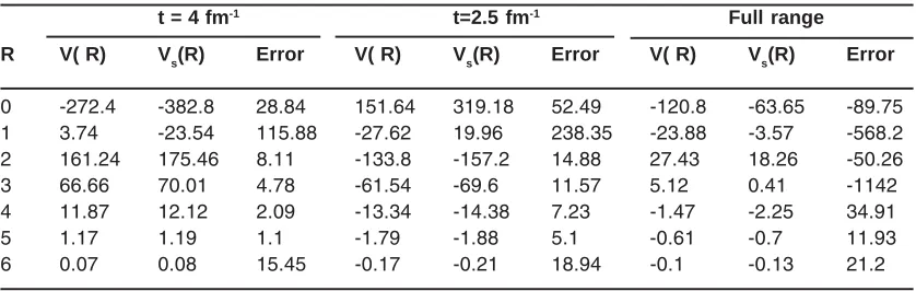
Table 5(c): Is the same as Table (4c) but using density dependent BDM3Y₃ force

0 -272.4 -382.8 28.84 151.64 319.18 52.49 -120.8 -63.65 -89.75

1 3.74 -23.54 115.88 -27.62 19.96 238.35 -23.88 -3.57 -568.2

2 161.24 175.46 8.11 -133.8 -157.2 14.88 27.43 18.26 -50.26

3 66.66 70.01 4.78 -61.54 -69.6 11.57 5.12 0.41 -1142

4 11.87 12.12 2.09 -13.34 -14.38 7.23 -1.47 -2.25 34.91

5 1.17 1.19 1.1 -1.79 -1.88 5.1 -0.61 -0.7 11.93

6 0.07 0.08 15.45 -0.17 -0.21 18.94 -0.1 -0.13 21.2

we note that the density dependent contribution of the NN force contains the sum (

2

1

ρ

+

). This term is calculated usually by assuming that the value of (

2

1

ρ

+

) corresponds to the values of densities at the positions of the interacting nucleons (

)

(r

ρ

)

(r

ρ

₁ ₁

+

₂ ₂

). Another way is to evaluate the sum of the two densities at a point midway between the interacting nucleons so that it is expressed as

the sum

⎟ ⎠ ⎞ ⎜

⎝

⎛ ₊ ₊ ₋

) s 2 1 r (

ρ

) s 2 1 r (

ρ₁r₁ r ₂r₂ r

.If the interacting nuclei have large mass numbers the two approaches produce almost the same value of the density and the effect of s-dependence becomes larger. For strong overlap between light nuclei there is a large

chance that the total density ⎟

⎠ ⎞ ⎜

⎝

⎛ ₊ ₊ ₋

) s 2 1 r ( ρ ) s 2 1 r (

ρP 1 T 2

r r r r

(11)

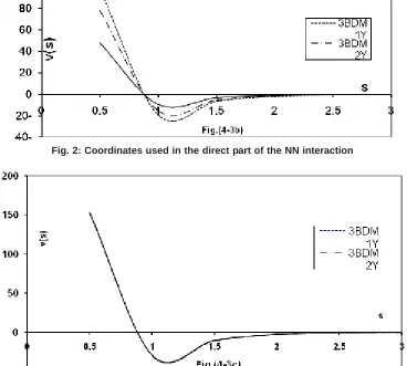
Fig. 1: Coordinates used in the exchange part of the nucleus-nucleus interaction

Fig. 2: Coordinates used in the direct part of the NN interaction

(12)

Fig. 3(b) Is the same as Fig.(3a) but at constant σσσσσ= σσσσσ₀ fm-3

Fig. 3(c) Is the same as Fig.(3a) but at constant σσσσσ= 0.5ñ₀ fm-3

(13)

densities. Since the NN interaction is of the form, )

αρ -cv(s)(1 ρ)

v(s, = β , the appearance of s in

ρ

produces a NN interaction potential value small compared to the case when s-dependence is ignored. So, we expect that the HI potential calculated, for small R-values, using the form

(

ρ_P(rr₁)+ρ_T(rr₂)

)

in NN force is enhanced compared

to that calculated by including

s

r

in the total density. This appears clearly for the NN force ranges 0.25 and 0.4 fm presented on tables (4) and (5) where the

α

-α

potential V(R) and V_s(R) are calculated

receptively using the expressions

(

ρ_P(rr₁)+ρ_T(rr₂)

)

and

⎟ ⎠ ⎞ ⎜

⎝

⎛ ₊ ₊ ₋ _s₎

2 1 r (

ρ

) s 2 1 r (

ρP 1 T 2

r r r r

in the NN force density dependent term. Table (4) shows the potential calculated, at different separation distances R, using the BDM3Yn(n=1,2,3) -Reid NN forces .The table

contains the contributions of V(R) and V_s(R)

resulting from one Yukawa term with ranges 0.25 and 0.4 fm. and the same quantities calculated using NN force which contains the two ranges. Table (5) is the same as table (4) except it is for Paris type of force. The tables show that for one Yukawa is greater than, in most cases, for small R values. The error in neglecting the s-dependence increases as the range of NN force increases. This is reasonable for all separation distances between the two interacting nuclei. For, calculated using one Yukawa term in becomes smaller than .This is because as the separation distance between the two nuclei increases, the sum has large chance to be greater than during the integration process on the volume elements. This behavior is clear on tables (4) and (5), for the two separate Yukawa ranges 0.25 and 0.4 fm. When the two Yukawa terms are combined

together to for m M3Y-force, V(R) and V_s(R)

becomes different in behavior than the case of single Yukawa term. For, V(R) is less repulsive or more attractive compared to V(R, s) .In the surface and tail regions V(R) becomes less attractive or

more repulsive than V_s(R).

For Reid type of NN force, the magnitude of the percentage error is too large in the inner region while it is smaller in the surface and tail regions. For Paris force the situation is different,

the error in the total potential is too large at R=3fm.This large value of error is accompanied by small error values for the two Yukawa ranges 0.25 and 0.4 fm. This can be interpreted if we remember that the direct part of HI potential calculated using Paris NN force is repulsive at small R values then it passes through zero and becomes attractive. For the distance R=3 fm. the value of potential is too

small and any small change between V(R) and V_s(R)

produces large value of error. The difference

between V(R) and V_s(R) together with the difference

in HI potential due to change of NN force can be understood from Figs.(3) and (4) .

Fig.(3) shows the variation of the direct part of Reid NN forces with the distance between the two interacting nucleons calculated at three different values of density. These values are , and where is the - particle density at the center of the nucleus. Fig.(4) is the same as Fig.(3) except it is for Paris interaction .It is noted that strong variation of NN force with internucleon distance produces

large difference between V(R ) and V_s(R) .This is

clear on table (4) for BDMN3Y_n(n=1 ,2,3) forces at

where Fig.(3) shows rapid variation of v(s, ) with

the distance s for BDM3Y₃ and slow variation for

BDM3Y₁ .This interprets the large error in neglecting

the s-dependence produced at R<2 fm. for BDM3Y₃

Reid force. In the surface and tail regions() the error produced by neglecting s-dependence is less than 50% because the shape of NN forces at and are almost similar and does not vary strongly with s. For Paris type of NN force shown in Fig.(4) , the

direct part of BDM3Y₃ force is strongly attractive

for s < 1 fm. then it becomes repulsive. This produces highly attractive HI potential in the inner region for range 0.25 fm. and repulsive potential for

range 0.4 fm. The strong variation of BDM3Y₃ for

small s-values Fig(4a) produces large error between V(R ) and V (R ,s) in the inner region . As the distance R increases Fig.(4b) and (4c) show that v(s, ) becomes highly repulsive at small s-values and weakly attractive for .This produces weakly attractive total potential in the tail region table(5).

REFERENCES

1. R.K.Gupta,W.Scheid and W.Greiner, Phys.

Rev. Lett. 35(9): 353 (1974).

2. D.Scharnweber,W.Greiner and W.Mosel,

(14)

3. W.Greiner and W.Scheid, J. Phys. Paris 32(C6): 91 (1971).

4. H.Holm and W.Greiner, Nucl. Phys.A195:

333 (1972) .

5. R.Sar tor,A.Faessler,S.B.Khodkikar and

Kerwald, Nucl. Phys. A354,467(1981) .

6. D.M.Brink and F. Stancu, Nucl. Phys.

A243,175(1975); F.Stancu and D.M.Brink, A270: 236 (1976) .

7. M.Ismail, M.Rashdan, A.Faessler, R.linden,

N.Ohtsuk and W.Wadia, ibid A490: 715 (1989); M.Ismail, H. Abozahra, Phs. Rev. C53:53(1996) .

8. J.Blucki,J.Randrup ,W.J.Swiatecki , and

C.F.Tsang ,Ann. Phys.(NY), 105: 427 (1977).

9. G.R.Satchler and W.G.Love, Phys. Rep.55:

183 (1979).

10. J.W.Negele and D.Vautherin, Phys. Rev. C5:

1472 (1972), C11: 1032(1975).

11. Dao T.khoa, Nucl.Phys. A486 169 (1988).

12. Dao T.Khoa and W.Von Oertzen, Phys.Lett.

304: 8 (1993).

13. Dao T.Khoa and W.Von Oertzen and H.G.

Bolhen,Phys. Rev. Cha: (1994)1652.

14. Dao T.Khoa and W.Von Oertzen, Phys. Lett.

B 342: 6 (1995).

15. Dao T.Khoa et.al., Phys. Rev. Lett.74: 134

(1995).

16. Dao T.Khoa ,G.R.Satchler and W.Von

Oertzen, Phys.Rev. C56: 954 (1997).

17. B.Sinha,Phys.Rep. 20: (1975).

18. A.K.Chaudhuri,D.N.Basu and B.Sinha, Nucl.

Phys.A43: 415 (1985); A.K.Chaudhuri and

B.Sinha ,Nucl.Phys. A455: 169 (1986).

19. S.Misicu and W.Greiner, Phys. Rev.C66:

044606 (2002).

20. M.El.Azab Farid and G.R. Satchler, Nucl.

Phys.A438: 525 (1985).

21. D.A. Goldberg et al.,Phys. Rev. C7: 1938

(1973).

22. H.G. Bohlen et al., Z. Phys. A308: 21 (1982).

23. H.G. Bohlen et al., Z. Phys. A322: 241 (1985).

24. E. Stiliais et al., Phys. Lett. B223: 291 (1989).

25. G.Bertsch et.al, Nucl. Phys. A284: 199

(1977).

26. A.M.Kobos et al.,Nucl. Phys. A384: 65 (1982);

A.M.Kobos et al.,Nucl. Phys. A425: 205

(1984).

27. M.E.Brandon and G.R.Satchler, Phys. Rep.

285: 14 (1997).

28. W.G.Love and L.W.Owen,Nucl. Phys. A239:

74 (1975).

29. M.Golin,F.petrovich and D.Robson,

Phys.Lett. B64: 253 (1976).

30. M.E. Brandan, M.Rodigueg-Villafuerte and

A.Ayala, Phys. Rev. C41: 1520 (1990).

31. M.E. Brandan and G.R. Satchler Phys. Lett.

B256: 311 (1991).

32. H.J.Krappe,J.R.Nix,and A.J.Sierk, Phys.

Rev.C20: 992(1979).

33. M.M. Osman, Balkan Phys. Lett. 6: 25 (1998).

34. M. Ismail,M.M. Osman and F. Salah,Phys.

Lett. B378: (1996)40;M. Ismail, F. Salah and M.M. Osman,Phys. Rev.C54: 3308 (1996).

35. B.Sinha, and S.A. Moszkowski, Phys. Lett.

B81: 289 (1979).

36. A.Faessler,W.H.Dickoff,M.Trefz and M.Trefz

and M.Rhoades- Brown, Nucl. Phys. A 428: 2710 (1984).

37. D.A.Saloner and C.T. Toepffer, Nucl. Phys.

A283: 108 (1977).

38. M.Ismail, A.Y.Ellithi, Choas Solitons and

Fractals, 14(9): 1425 (2002)

39. X.Campi,and A.Bonyssy, Phys. Lett. B73:

263 (1978)

40. J.Phys.G2: 285 (1976)

41. S.Sartor and F.I.Stancu, Phys. Rev.C29:

1756 (1984).

42. L.G.B.Goldfarb, P.Nagel, Nucl. Phys.A34: 494