Blending Learning and Inference in Conditional Random Fields

Blending Learning and Inference in Conditional Random

Fields

Tamir Hazan [email protected]

Technion - Israel Institute of Technology Technion City,

Haifa, 3200, Israel

Alexander G. Schwing [email protected]

Electrical and Computer Engineering and Coordinated Science Laboratory, University of Illinois at Urbana-Champaign

Urbana, IL 61801

Raquel Urtasun [email protected]

University of Toronto 40 St. George Street, Toronto, ON, M5S 2E4

Editor:Sebastian Nowozin

Abstract

Conditional random fields maximize the log-likelihood of training labels given the train-ing data, e.g., objects given images. In many cases the traintrain-ing labels are structures that consist of a set of variables and the computational complexity for estimating their likelihood is exponential in the number of the variables. Learning algorithms relax this computational burden using approximate inference that is nested as a sub-procedure. In this paper we de-scribe the objective function for nested learning and inference in conditional random fields. The devised objective maximizes the log-beliefs — probability distributions over subsets of training variables that agree on their marginal probabilities. This objective is concave and consists of two types of variables that are related to the learning and inference tasks respectively. Importantly, we afterwards show how to blend the learning and inference pro-cedure and effectively get to the identical optimum much faster. The proposed algorithm currently achieves the state-of-the-art in various computer vision applications.

1. Introduction

Learning and inference of structured models drives much of the research in machine learning applications, from computer vision and natural language processing to computational biol-ogy. Examples include object detection (e.g., by Felzenszwalb et al. (2010)), parsing (e.g., by Koo et al. (2010)), or protein design (e.g., by Sontag et al. (2008)). The inference prob-lem in these cases involves assessing the likelihood of labelings, whether outlined objects, parse trees, or molecular structures. The learning procedure searches for the parameters that maximize the likelihood of the training set.

can be computationally expensive since the label space of real-world problems is usually exponential in the size of its variables.

When the label structure corresponds to a tree, exactly inferring the likelihood of the training labels can be done in time, linear in the number of variables using sum-product belief propagation as a subroutine. We refer to this approach as nested learning and infer-ence. In contrast, when the label structure corresponds to a general graph, we cannot infer the likelihood exactly. However nested learning and inference can still be applied using ap-proximate inference algorithms such as convex sum-product belief propagation (Wainwright et al., 2005; Heskes, 2006; Meltzer et al., 2009; Hazan and Shashua, 2010). Nevertheless, the approximate inference algorithms might be computationally expensive to be used as a nested subroutine of the learning algorithm.

In this article we suggest to interleave optimization of learning parameters with opti-mization of inference parameters. We call this approach blending learning and inference in CRFs. For this end we propose an optimization program that maximizes log-beliefs, i.e., probability distributions over subsets of training variables that agree on their marginal probabilities. These beliefs are elements of the local polytope (Wainwright and Jordan, 2008). The log-beliefs objective is concave and consists of two types of variables that are related to the learning and inference tasks respectively. We are able to blend the learn-ing and inference procedures by alternatlearn-ing maximizations over the inference and learnlearn-ing variables. With blending we reach the nested learning-inference optimum much faster.

We also define loss-adjusted beliefs to integrate prior knowledge about the desired in-ference as well as a parameter that controls the smoothness of the beliefs. In the past and partly due to its efficiency, the presented machine learning algorithm was shown to improve the state-of-the-art in various computer vision tasks, including 2D scene understanding (Yao et al., 2012), 3D scene understanding (Lin et al., 2013), shape reconstruction (Salzmann and Urtasun, 2012), indoor scene understanding (Schwing et al., 2012a; Schwing and Urta-sun, 2012), depth estimation (Yamaguchi et al., 2012), flow estimation (Yamaguchi et al., 2013) and visual-language understanding (Fidler et al., 2013). This manuscript extends our previous work (Hazan and Urtasun, 2010) to high order setting while simplifying its theory and proofs. The code is publicly available onhttp://www.alexander-schwing.de/ projectsGeneralStructuredPredictionLatentVariables.php.

2. Related work

Learning log-beliefs extends the CRFs framework that maximizes the log-likelihood of con-ditional Gibbs distributions (cf. Lafferty et al. (2001); Lebanon and Lafferty (2002)). Gibbs distributions, also known as Markov random fields, are probability distributions that are defined on a product space using potential functions over subsets of variables. Gibbs prob-ability models often consider exponentially many possible assignments for these variables. In this case, approximate inference methods are used in a black box manner to estimate the gradient and the objective of CRFs, resulting in the nested learning-inference algorithm illustrated in Figure 1. Nested learning-inference algorithms are successfully dealing with real-world problems, e.g., (Levin and Weiss, 2006) in computer vision, (Yanover et al., 2007) in computational biology and (Sutton and McCallum, 2009) in language processing to name a few.

The current work extends and simplifies our previous work (Hazan and Urtasun, 2010). We simplify the learning objective while formulating it as the maximization of log-beliefs, which are pseudo-marginal probabilities of the Gibbs distribution. We extend the learning procedure while considering pseudo-marginals of Gibbs distributions on any subset of its variables. In the last couple of years, the presented machine learning algorithm was shown to improve the state-of-the-art in various computer vision tasks: Considering outdoor scene understanding (Yao et al., 2012), each (super)pixel is represented by a variable of the Gibbs model and its possible assignments correspond to discrete semantic label, e.g., person, car, tree and so on. Our learning algorithm estimates the parameters that maximize the probability of the training data per variable (i.e., pixel and its observed object) and subsets of variables (e.g., neighborhood of pixels and their observed objects). Considering indoor scene understanding (Schwing et al., 2012a; Schwing and Urtasun, 2012; Lin et al., 2013) each wall or a 3D object in the room is represented by a subsets of variables and our learning algorithm estimates the position of these objects while maximizing likelihood of these subsets within the training data. In depth estimation and optimal flow (Yamaguchi et al., 2012, 2013) the variables of the Gibbs models are either continuous or discrete. The continuous variables correspond to the possible hyperplanes that either explain the depth or the optical flow of the super pixels in the training images. The discrete variables maintain consistency between adjacent super pixels. Our learning algorithm estimates the probable hyperplanes and their spatial relations in the training data.

Our approach suggests to blend the inference and learning steps and reach the same optimum as nested approaches while being at least an order of magnitude faster. Blending helps the algorithm to avoid computationally expensive inference algorithms when learning parameters w that are far from optimal. Similar observations have been made in the con-text of coordinate descent by Tappenden et al. (2013). Other approaches for blending CRFs appear are developed by Domke (2011). Lemma 3 describes how to infer non-consistent be-liefs. These beliefs are different from the beliefs that are usually derived during the runtime of approximate inference algorithms. The theoretical characterization of the optimal points for the learning-inference procedures are described by Wainwright (2006); Wainwright et al. (2003).

observed ones (cf. (Taskar et al., 2004; Tsochantaridis et al., 2004; Collins, 2002)). The ideas of blending learning and inference in structured SVMs also appear in (Taskar et al., 2005; Anguelov et al., 2005). In contrast, our work focuses on blending learning and inference when maximizing log-probabilities. Nevertheless, our loss-adjusted beliefs may describe a probabilistic alternative to blended learning in structured-SVMs. When setting the counting numbers cr = 0, we effectively work with zero-one probabilities (i.e., max-beliefs) thus we recover the algorithm of Meshi et al. (2010).

3. Background

Log-likelihood learning in structured models involves data instancesx∈ X and their labels y∈ Y. The structure is incorporated into the labels which may refer to sequences, grids, or other high-dimensional objects. For every data instance x, its possible labels are described by a set of feature functions φk : X × Y → R, k ∈ {1, . . . , K}. A linear combination of the K features is used to score the different labels y ∈ Y using the parameters w ∈ RK. Formally we obtain the scoreθ(y;x, w) of a label via

θ(y;x, w) =X k

wkφk(x, y).

The real valued score is mapped to the probability scale via the Gibbs distribution:

p(y|x;w)∝exp(θ(y;x, w)). (1)

Within the CRF framework, the goal is to learn the parameters of the potential functions to maximize the conditional likelihood of the training data (x, y)∈ S:

max w

X

(x,y)∈S

logp(y|x;w)−C 2kwk

2

2. (2)

The regularization term is sometimes considered as a Gaussian prior over the parameters w. The regularized likelihood of CRFs is a concave and smooth function and its optimal parameters may be attained by gradient ascent. The gradient measures the disagreements between the inferred distribution over labels and the groundtruth training labels, i.e.,

∂ logp(y|x;w) ∂wk

=X ˆ y∈Y

p(ˆy|x;w)φk(x,y)ˆ −φk(x, y). (3)

The computational complexity of CRFs is governed by inference, which amounts to evalu-ating the probability p(ˆy|x;w) for computing the objective and the gradient.

We consider cases in which the labelsy∈ Y aren-tuples, i.e.,y = (y1, ..., yn), and hence the configuration space is exponential inn. The features describe relations between subsets of elements r ⊂ {1, ..., n}, also called regions or factors. We denote by Rk the regions required to compute the feature φk(x, y). Importantly, the features are functions of their regions labels yr⊂ {y1, ..., yn}, i.e.,

φk(x, y1, ..., yn) =

X

r∈Rk

Thus the features define hypergraphs whose nodes represent the n labels indexes, and the regions R = ∪kRk correspond to its hyperedges. A convenient way to represent a hypergraph is by its region graph. A region graph is a directed graph whose nodes represent the regions and its direct edges correspond to the inclusion relation, i.e., a directed edge from node r to sis possible only if s⊂r. We adopt the terminology where the sets P(r) and C(r) represent all nodes that are parents and children of the noder, respectively.

The Hammersley-Clifford theorem (e.g., Lauritzen (1996)) asserts that the Gibbs dis-tributions p(ˆy|x;w) defined in Equation (1) correspond to a Markov random field (MRF) whose statistical independencies are described by the joint hypergraph. These indepen-dencies are determined by the Markov property: two nodes in the graph are conditionally independent when they are separated by observed nodes. Aji and McEliece (2001) show that whenever the region graph is bipartite and has no cycles, the Markov property provides a low dimensional representation of the Gibbs distribution using its marginal probabilities p(ˆyr|x;w) =Pyˆ\yˆrp(ˆy|x;w), namely

p(ˆy|x;w) = Y r∈R

p(ˆyr|x;w)1−|P(r)|. (5)

In such cases the inference step, i.e., estimating the probabilities p(ˆy|x;w) can be per-formed efficiently using message-passing algorithms. When the region graph has no cycles it is bipartite, therefore it has two types of regions: outer regions, i.e., regions that are not contained by other regions, and inner regions. To differentiate between those regions we denote outer regions by α and inner regions by i. In this case, one can use the be-lief propagation algorithm to efficiently infer the marginal probabilities without performing exponentially many operations:

Algorithm 1 Sum-product belief propagation

SetK_r={k:r ∈ R_k}. For every (x, y), w set θr(ˆyr) =Pk∈Krwkφk,r(x,yˆr).

Repeat until convergence:

µα→i(yi) = log

P

yα\yiexp (θα(yα) +

P

j∈C(α)\iλj→α(yj))

λi→α(yi) =θi(yi) +Pβ∈P(i)\αµβ→i(yi) Output:

bi(yi)∝exp θi(yi) +P_α∈P(i)µα→i(yi)

bα(yα)∝ θα(yα) +Pi∈C(α)λi→α(yi)

The marginal probabilities p(ˆyr|x;w) appear as the beliefsbr(ˆyr). In general, when the region graph has cycles, the belief propagation algorithm is no longer guaranteed to output the marginal probabilities. Nevertheless, when it converges it provides beliefs that agree on their marginal probabilities, namelyP

yα\yibα(yα) =bi(yi). In some cases the belief

possi-ble explanation for this behavior comes from the fact that the belief propagation algorithm iterates the stationary points of a non-convex objective called the Bethe free energy (Yedidia et al., 2005). Recently, in an extensive effort to derive converging belief propagation type algorithms, the non-convex Bethe free energy was replaced by convex free energies while introducing nonnegative counting numbers cr that replace the Bethe coefficients. Conse-quently, the belief propagation algorithm was replaced by block coordinate descent over the dual program (Heskes, 2006; Meltzer et al., 2009; Hazan and Shashua, 2008). These dual block coordinate descent algorithms belong to the family of the norm-product belief propagation algorithms:

Algorithm 2 Norm-Product Belief Propagation Set ˆci =ci+P_α∈P(i)cα. Repeat until convergence:

µα→i(yi) =cαlog

P

yα\yiexp (θα(yα) +

P

j∈C(α)\iλj→α(yj))

cα

λi→α(yi) = c_cˆα

i

θi(yi) +P_β∈P(i)µβ→i(yi)

−µα→i(yi)

Output:

bi(yi)∝exp θi(yi) +P_α∈P(i)µα→i(yi)

1/ˆci

bα(yα)∝exp θα(yα) +P_i∈C(α)λi→α(yi)

1/cα

The norm-product algorithm, illustrated in Algorithm 2, reduces to belief propagation when setting its coefficients to cr = 1− |P(r)|, namely, the Bethe counting numbers. We refer the interested reader to (Wainwright and Jordan, 2008) for more details.

The norm-product algorithm iterates over the fixed point solutions for the variational problem

arg max b∈L(G)

X

r,yr

br(yr)θr(yr) +

X

r

crH(br). (6)

The set L(G) is known as the local polytope, and contains probability distributions br(yr) that agree on their overlapping variables, i.e.,

L(G) =

n

br(yr) : br(yr)≥0,

X

yr

br(yr) = 1, ∀p∈P(r)

X

yp\yr

bp(yp) =br(yr)

o

. (7)

Throughout this work we refer to elements in the local polytope as beliefs.

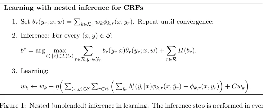
Learning with nested inference for CRFs

1. Setθr(yr;x, w) =Pk∈Krwkφk,r(x, yr). Repeat until convergence:

2. Inference: For every (x, y)∈ S:

b∗ = arg max b(·|x)∈L(G)

X

r∈R,yr∈Yr

br(yr|x)θr(yr;x, w) +

X

r∈R

H(br).

3. Learning:

wk←wk−η

P

(x,y)∈S

P

r∈R

P

ˆ yrb

∗

r(ˆyr|x)φk,r(x,yˆr)−φk,r(x, yr)

+Cwk

.

Figure 1: Nested (unblended) inference in learning. The inference step is performed in every iteration. The learning step improves the parameters till learning is attained. η is typically referred as the learning rate and may be set as 1/√t, where t is the iteration index. The abbreviationb∈L(G) describes conditional beliefsb(·|x) for everyx∈S. Each of these conditional beliefs is in the local polytope, as defined in Equation (7).

the gradient is computationally demanding and this method has not been used widely (see Section 2 for more details). In the following we explore duality to provide the means to blend the learning and inference tasks efficiently.

4. Blending learning and inference

Log-likelihood of Gibbs distributions, as defined in Equation (1) with potentialsθ(y;x, w) that are linear functions of their parametersw, results in a concave program. When using nested (unblended) inference, the learning algorithm executes a concave program for infer-ring beliefs about its marginal probabilities that are required for computing its gradient. Our main result explicitly defines the concave program whose optimal solutions are the limit points of the nested learning and inference algorithm that is shown in Figure 1. Using this characterization we are able to derive an algorithm that blends the learning and infer-ence steps. Consequently it is orders of magnitude faster than the nested algorithm that uses inference as a black-box algorithm. Since our blended algorithm optimizes a concave program, it is guaranteed to reach the same optimum as the nested algorithm.

Theorem 1 The limit points of the nested inference and learning algorithm in Figure 1 are described by the optimal points of the following concave program maximizing log-beliefs:

max w,λ

X

(x,y)∈S

X

r∈R

logbr(yr|x;w, λ)− C

2kwk 2

s.t br(yr|x;w, λ)∝exp

θr(yr;x, w) +

X

c∈C(r)

λc→r(yc;x)−

X

p∈P(r)

λr→p(yr;x)

Proof The theorem replaces maximization overb∈L(G) with maximization overλ. De-coupling the maximizations takes the form maxwP_(x,y)∈S maxλ{

P

r∈Rlogbr(yr|x;w, λ)}

. In the following we show how to derive the result from Lagrange optimality conditions (KKT):

λ∗ = arg max λ

X

r∈R

logbr(yr|x;w, λ)

b∗ = arg max b∈L(G)

X

r∈R,yr∈Yr

br(yr|x)θr(yr;x, w) +

X

r∈R

H(br)

=⇒b∗_r(yr|x)∝exp

θr(yr;x, w) +

X

c∈C(r)

λ∗_c→r(yc;x)−

X

p∈P(r)

λ∗_r→p(yr;x)

(8)

Using the above Lagrange optimality conditions, the theorem follows since the inference nested within the learning algorithm applies gradient ascent to the following program:

max w

X

(x,y)∈S max

λ {

X

r∈R

logbr(yr|x;w, λ)}

−C 2kwk

2 _{= max} w

X

(x,y)∈S

X

r∈R

logb∗_r(yr|x)− C

2kwk 2_.

Equation (8) states the Lagrange optimality conditions for likelihood maximum-entropy type duality. Consider the constrained inference algorithm in Figure (1) and the Lagrange multipliers λr→p(yr;x, w) for the marginalization constraints Pyp\yrbp(yp|x) =

br(yr|x). Its corresponding Lagrangian isL(b, λ) =Pr,yrbr(yr|x)θr(yr;x, w, λ) +

P

rH(br) where θr(yr;x, w, λ) = θr(yr;x, w) +Pc∈C(r)λc→r(yc;x) −Pp∈P(r)λr→p(yr;x). Its dual function isq(λ) = maxbL(b, λ) whilebr(yr|x) are subject to probability constraints. Con-jugate duality between the entropy function and the log-partition function (cf. Wainwright and Jordan (2008)) implies that q(λ) = P

rlog(

P

yrexp(θr(yr;x, w, λ))). Since strong

du-ality between the entropy and the log-partition function holds, its Lagrange optimdu-ality conditions imply

λ∗ = arg min λ

X

r∈R

log X yr

exp θr(yr;x, w, λ)

.

The theorem then follows sinceP

r∈R

P

p∈P(r)λr→p(yr;x)−Pr∈R

P

c∈C(r)λc→r(yc;x)≡0 thereforeP

rlogb∗r(yr|x) =−q(λ∗) and the Lagrange optimality conditions in Equation (8) hold. Thusb∗_r(yr|x) can be replaced by its re-parametrization _Z1_rexp(θr(yr;x, w, λ∗)), with Zr =Pyˆrexp(θr(ˆyr;x, w, λ

∗_)).

The maximum log-beliefs program describes the variational landscape of nested inference in learning. Thus it can be used to measure the step-size η in Figure 1. For example, the Armijo rule that determines the step size according to the variational neighborhood results in a faster convergence per iteration than using a fixed learning rate.

to blend learning (optimization w.r.t. w) with incomplete inference steps (optimization w.r.t.λ) that derive beliefsbr(yr|x;w, λ) that not necessarily agree on their marginal prob-abilities, i.e., P

yp\yrbp(yp|x;w, λ) = br(yr|x;w, λ). Such an approach is computationally

favorable since it does not require to perform a complete inference step for initial learning parameters. Concavity ensures that blending reaches the maximum log-beliefs optimum thus it guarantees to derive consistent beliefs upon convergence.

Performing block coordinate descent on the maximum log-beliefs program in Theorem 1 requires minimizing a block of variables while holding the rest fixed. We begin by describing how to infer the optimal set of variables λr→p(yr;x) that are related to a region and its parents in the graphical model.

Lemma 2 Blended inference: Consider the program given in Theorem 1. For a given

region r, the optimal inference parameters λ∗_r→p(yr;x), for every p∈ P(r), yr ∈ Yr, x∈ S,

when fixing all other λtakes the following form:

µp→r(yr;x) = log

X

yp\yr

exp θp(yp;x, w) +

X

c∈C(p)\r

λc→p(yc;x)−

X

p0_∈P(p)

λp→p0(ˆy_p;x)

λ∗_r→p(yr;x) =

θr(yr;x, w) +Pc∈C(r)λc→r(yc;x) +Pp0_∈P(r)µp0_→r(y_r;x)

1 +|P(r)| −µp→r(yr;x)

Proof The maximum log-beliefs program in Theorem 1 is smooth, concave and uncon-strained as a function of λ, therefore the optimum is achieved when the gradient vanishes. Setting

θr(yr;x, w, λ) =θr(yr;x, w) +

X

c∈C(r)

λc→r(yc;x)−

X

p∈P(r)

λr→p(yr;x) (9)

and br(yr|x;w, λ) ∝exp(θr(yr;x, w, λ)), the gradient with respect toλr→p(yp;x) takes the form

∂P

(x,y),rlogbr(yr|x;w, λ) ∂λr→p(yr;x)

= X

yp\yr

bp(yp|x;w, λ)−br(yr|x;w, λ).

The optimal dual variables are those for which the gradient vanishes, i.e., the corre-sponding beliefs agree on their marginal probabilities. When setting µp→r(yr;x) as above, the marginalization ofbp(yp|x;w, λ) satisfies

X

yp\yr

bp(ˆyp|x;w, λ)∝exp µp→r(yr;x) +λr→p(yr;x)

.

Therefore, by taking the logarithm, the gradient vanishes whenever the beliefs numerators agree up to an additive constant:

X

yp\yr

bp(yp|x;w, λ∗)−br(yr|x;w, λ∗) = 0⇐⇒µp→r(yr;x) +λ∗r→p(yr;x) =θr(ˆyr;x, w, λ∗).

The right hand side of the condition almost characterizes completely the optimal variables λ∗_r→p(yr;x) by λr∗→p(yr;x) = θr(ˆyr;x, w, λ∗)−µp→r(yr;x). Unfortunately, θr(ˆyr;x, w, λ∗) depends onP

p∈P(r)λ

∗

To complete the proof we require to replaceP

p∈P(r)λ∗r→p(yr;x) with another quantity that does not depend on λ∗_r→p(yr;x) for everyp∈P(r) and yr∈ Yr.

To isolate this quantity we sum both sides of the equality µp→r(yr;x) +λ∗r→p(yr;x) = θr(ˆyr;x, w, λ∗) with respect top∈P(r), thus we are able to obtain

(1 +|P(r)|) X p∈P(r)

λ∗_r→p(yr;x) =|P(r)|(θr(yr;x, w) +

X

c∈C(r)

λc→r(yc;x))−

X

p∈P(r)

µp→r(yr;x)

Plugging it into the above equation results in the desired block dual ascent update rule.

One can verify that since the program is not strictly concave inλ, the optimal solutions can be achieved for every additive shift of λr→p(yr;x). The above lemma describes an analytic solution for the optimalλr→p(yr;x), that are computed in the block coordinate steps of the algorithm. In practice, block coordinate descent with analytic steps provides a significant speedup over conventional gradient methods and can be parallelized and distributed easily, as shown by Schwing et al. (2011).

A learning step updates the weights w so as to maximize the log-beliefs. When using blended inference, the beliefs are not required to agree on their marginal probabilities. However, they are governed by the concave program in Theorem 1. Its concavity guarantees that these beliefs agree on their marginals at the optimum.

Lemma 3 Blended learning: Consider the program given in Theorem 1. The gradient

of its objective function with respect to wk takes the form:

X

(x,y)∈S

X

r∈Rk

X

ˆ yr∈Yr

br(ˆyr|x;w, λ)φk,r(x,yˆr)−φk,r(x, yr)

+Cwk.

Proof We let

logbr(yr|x;w, λ) =θr(yr;x, w, λ)−log

X

ˆ yr

exp θr(ˆyr;x, w, λ)

.

The theorem follows by noting thatθr(yr;x, w) =P_k∈Krwkφk,r(x, yr), recalling the

defini-tion ofθr(yr;x, w, λ) in Equation (9) and thatbr(ˆyr|x;w, λ) which is defined in Theorem 1 is the gradient of its log-partition function, i.e., logP

ˆ

yrexp θr(ˆyr;x, w, λ)

.

The computational complexity of the gradient depends on the structure of the features, es-pecially the number of regions and their labels. Our framework prefers features with small regions and reasonable number of labels. Another computational issue relates to the step size η for increasing the objective along the gradient of wk. In general, the gradient up-dates verify that the chosen step sizeη reduces the objective. Theoretically, we can use the fact that the gradient is Lipschitz continuous to predetermine a step size that guarantees ascent. In practice it gives worse performance than searching for a step size depending on the gradient and the objective at any given point.

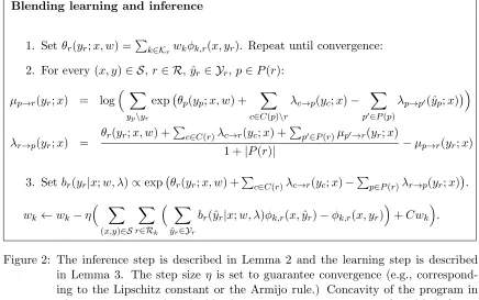
Blending learning and inference

1. Setθr(yr;x, w) =Pk∈Krwkφk,r(x, yr). Repeat until convergence:

2. For every (x, y)∈ S,r ∈ R, ˆyr∈ Yr,p∈P(r):

µp→r(yr;x) = log

X

yp\yr

exp θp(yp;x, w) +

X

c∈C(p)\r

λc→p(yc;x)−

X

p0_∈P(p)

λp→p0(ˆy_p;x)

λr→p(yr;x) =

θr(yr;x, w) +P_c∈C(r)λc→r(yc;x) +

P

p0_∈P(r)µ_p0_→r(y_r;x)

1 +|P(r)| −µp→r(yr;x)

3. Setbr(yr|x;w, λ)∝exp θr(yr;x, w) +

P

c∈C(r)λc→r(yc;x)−

P

p∈P(r)λr→p(yr;x)

.

wk←wk−η

_X

(x,y)∈S

X

r∈Rk

_X

ˆ yr∈Yr

br(ˆyr|x;w, λ)φk,r(x,yˆr)−φk,r(x, yr)

+Cwk

.

Figure 2: The inference step is described in Lemma 2 and the learning step is described in Lemma 3. The step size η is set to guarantee convergence (e.g., correspond-ing to the Lipschitz constant or the Armijo rule.) Concavity of the program in Theorem 1 ensures that the blending converges to consistent inferred beliefs, see Theorem 4.

they do not change before optimizing the learning parametersw. We refer to this approach in Figure 1 as nested inference within learning since it performs the approximate inference heuristic described in Section 3 as a black-box solver. Nested learning and inference is computationally unfavorable in general as it requires to infer λ till convergence for every gradient step for learningw. Since concavity ensures that the maximization does not depend on the order of the maximizing steps, it also provides a principled way to blend the learning and inference steps. Particularly, it may learn the w parameters using inferred beliefs br(yr|x;w, λ) ∝exp(θr(yr, x, w, λ)) that do not agree on their marginal probabilities. For this purpose our algorithm infers the parametrized beliefsdifferentlythan the (outer) beliefs that are computed by the nested learning algorithm in Figure 1. This blending property is important in practice, since shortly upon initialization, where the given parameters w are far from the optimum, it is not advisable to spend time on computing consistent beliefs. Figure 2 summarizes the inference-learning blending algorithm.

change the objective value, hence the algorithm can generate a monotonically decreasing unbounded sequences. Convergence to the optimum holds by convex duality:

Theorem 4 The learning-inference blending algorithm in Figure 2 for log-beliefs maximiza-tion is guaranteed to converge. Moreover, the value of its objective is guaranteed to converge to the global maximum, and its sequence of beliefs are guaranteed to converge to consistent beliefs that are the unique solution of the dual program

min z,br

X

(x,y)∈S

1 2Ckzk

2₋X

r∈R

H(br)

subject to br(ˆyr|x)≥0,

X

ˆ yr

br(ˆyr|x) = 1, br(ˆyr|x) =

X

ˆ yp\yˆr

bp(ˆyp|x)

zk=

X

(x,y)∈S

X

r∈Rk

X

ˆ yr

br(ˆyr|x)φk,r(x,yˆr)−φk,r(x, yr)

Proof The update rules in Figure 2 iteratively apply the block coordinate ascent rules in Lemmas 2 and 3 thus monotonically increase the primal objective in Theorem 1. This program is concave thus it is bounded by its dual program, therefore the value of its objective is guaranteed to converge. To derive the dual program we construct the Lagrangian

L(w, λ, b) = −C 2kwk

2₊X

k wk(

X

(x,y)∈S,r∈Rk

φk,r(x, yr))

− X (x,y),r

log X ˆ yr

exp(θr(ˆyr;x) +

X

c∈C(r)

λc→r(ˆyc;x)−

X

p∈P(r)

λr→p(ˆyr;x))

+ X

(x,y),r

X

ˆ yr

br(ˆyr|x)

θr(ˆyr;x)−

X

k

wkφk,r(x,yˆr)

.

The variables br(ˆyr|x) are the Lagrange multipliers for the equality constraints θr(ˆyr;x) =

P

kwkφk,r(x, yk). The dual program takes the form q(b) = maxw,λL(w, λ, b). Setting zk as above, since the k · k2 _{is the conjugate dual of k · k}2_{, the maximization over w takes} the form maxw{−C₂kwk2 −Pkwkzk} = ₂1_Ckzk2. To complete the derivation of the dual, the maximization over λ, for every (x, y) takes the form maxλ{Pr,yˆrbr(ˆyr|x)(θr(ˆyr;x)−

P

rlog(

P

ˆ

yrexp(θr(ˆyr;x) +

P

c∈C(r)λc→r(ˆyc;x)−

P

p∈P(r)λr→p(ˆyr;x)))}. This is the con-jugate dual of the log-partition function, which is known to be the entropy functionH(br). The mixing of the messages between the different regions results in the marginalization constraints in the dual program. An alternative proof for the conjugate duality between the re-parametrized log-partitions and entropies subject to marginalization constraints appears in the more generalized setting of Theorem 5.

Finally, since the dual is strictly convex subject to linear marginalization constraints and the linear moment constraints the convergence properties are a consequence of Tseng and Bertsekas (1987).

the function z2_k is strongly convex (e.g., Tseng and Bertsekas (1987)) and its gradient is Lipschitz continuous (e.g., Nesterov (2004)). In practice, Theorem 4 describes how to measure the convergence of the algorithm. Specifically, it may be derived from the primal objective value, the dual objective value or the beliefs themselves, as all these quantities converge. Unfortunately, the variablesλmight not converge, but if they do converge, their convergence point is optimal.

5. Blending learning and loss adjusted inference

Loss adjusted inference emerges from Support Vector Machines (SVMs) where a loss func-tion indicates preferences between different labels. In the following we consider nonnegative loss functions `r(yr,yˆr) ≥0 over subsets of variables, while `r(yr, yr) = 0. We suggest to augment our learned beliefs with loss adjusted probability models. Given a training example (x, y), we define the loss adjusted belief model to be

br(ˆyr|x;w, λ)∝exp

`r(yr,yˆr) +θr(ˆyr;x, w, λ)

.

Note that these beliefs should be conditioned overxas well as the vector`r(·, yr). However, to simplify the notation, we leave this conditioning implicit. The intuition for using the loss as a prior and for deriving loss adjusted beliefs is based on encouraging to learn parameters that decrease probabilities over labels with higher loss with respect to the training labels. The likelihood approach aims at maximizing the beliefsbr(yr|x;w, λ). Since the beliefs are probability distributions, it equivalently aims at minimizing the log-beliefs of all other as-signments, namely,br(ˆyr|x;w, λ) for every ˆyr6=yr. Since the loss`r(yr,yˆr) is a nonnegative function it implies that loss-adjusted maximum-likelihood learns parameters that better reduce scores of non-observed training labels, namely θr(ˆyr;x, w, λ) for any ˆyr 6= yr. The algorithms for maximizing loss adjusted beliefs models follow the derivations presented in Section 4, while replacing θr(ˆyr;x, w, λ) with θr(ˆyr;x, w, λ) +`r(ˆyr, yr). Letting z = (x, y) we introduce θr(ˆyr;z, w, λ) =θr(ˆyr;x, w, λ) +`r(ˆyr, yr).

The norm-product approach for inference may use counting numbers cr to control the peakedness of the beliefs, namely

br(ˆyr|x;w, λ, c)∝exp (θr(ˆyr;x, w, λ) +`r(ˆyr, yr))/cr

. (10)

Ascr→0 this distribution approaches a zero-one probably around the most likely structure, i.e., the desired loss adjusted prediction. Thus the following program blends learning with loss adjusted inference, as well as structured predictions (cf. Meshi et al. (2010)):

Theorem 5 Consider the loss adjusted beliefs given in Equation (10) and their maximum likelihood concave program:

max w,λ

X

z∈S

X

r∈R

cr·logbr(yr|x;w, λ, c)− C

2kwk 2_.

Setθˆr(yr;z, w) =θr(yr;x, w)+`r(yr,yˆr). Then, blending the following loss adjusted learning

cr>0.

µp→r(yr;x) =cplog

X

yp\yr

exp (ˆθp(yp;z, w) +

X

c∈C(p)\r

λc→p(yc;x)−

X

p0_∈P(p)

λp→p0(ˆy_p;x))/c_p

λr→p(yr;x) = cr

ˆ

θr(yr;z, w) +P_c∈C(r)λc→r(yc;x) +

P

p0_∈P(r)µp0_→r(y_r;x)

cr+P_p∈P(r)cp

−µp→r(yr;x)

wk ← wk−η

_X

(x,y)∈S

X

r∈Rk

_X

ˆ yr∈Yr

br(ˆyr|x;w, λ, c)φk,r(x,yˆr)−φk,r(x, yr)

+Cwk

.

Moreover, the beliefs converge to consistent beliefs that are the unique solution of the dual program

max br,u

X

(x,y),r

crH(br) +

X

ˆ yr

br(ˆyr|x)`r(yr,yˆr)

− 1 2Ckuk

2_,

subject touk=P(x,y),r

P

ˆ

yrbr(ˆyr|x)φk,r(x,yˆr)−φk,r(x, yr)

,br(ˆyr|x)≥0,Pyˆrbr(ˆyr|x) =

1 and br(ˆyr|x) =P_yˆp\yˆrbp(ˆyp|x).

Proof The update rule for w follows from Lemma 3 and the update rule for λ follows from Lemma 2. Since the program is unconstrained, the optimal λ is attained when the gradient vanishes, or equivalently P

yp\yrbp(yp|x;w, λ) = br(yr|x;w, λ), while br(·)

are the reparametrized beliefs. When setting µp→r(yr;x) as above, the marginalization ofbp(yp|x;w, λ) satisfyPyp\yrbp(ˆyp|x;w, λ)∝exp (µp→r(yr;x) +λr→p(yr;x))/cp

. There-fore, by taking the logarithm, the gradient vanishes whenever the beliefs numerators agree

µp→r(yr;x) +λr→p(yr;x) cp

= θr(yr;z, w) +

P

c∈C(r)λc→r(yc;x)−

P

p∈P(r)λr→p(yr;x) cr

Multiplying both sides by crcp and summing both sides with respect to p0 ∈ P(r) we are able to isolateP

p0_∈P(r)λ_r→p0(y_r;x). Plugin it into the above equation results in the desired

inference update rule, i.e., λr→p(yr;x) for which the partial derivatives vanish.

To prove the duality theorem we show that the primal program is the dual of its dual pro-gram using its Lagrangian. For everyr,yˆr, p∈P(r) we introduce the Lagrange multipliers λr→p(ˆyr;x) for the marginalization constraints br(ˆyr|x) = Pyˆp\yˆrbp(ˆyp|x). We also

intro-duce the Lagrange multiplierswkfor the constraintsuk=P_(x,y),r P_yˆrbr(ˆyr|x)φk,r(x,yˆr)− φk,r(x, yr)

. We let ∆r refer to the probability simplex constraining the beliefs br(ˆyr|x). Then the primal program takes the form p(λ, w) = maxbr∈∆r,uL(b, u, λ, w) which

decom-poses to P

z,rcrmaxbr∈∆r{H(br) +

P

ˆ

yrbr(yr|x)(`r(yr,yˆr) + θr(ˆyr;x, w, λ))/cr} +w

>_d+

maxu{w>u−₂1_Ckuk2}, wheredk are the empirical momentsdk=P(x,y),rφk,r(x, yr). Thus the primal is the sum of conjugate dual functions. The primal is then derived since the log-partition function is the conjugate dual of the entropy function and the conjugate dual of ₂1_Ckuk2 _is C

2kwk2. The form in the theorem is obtained since `r(yr, yr) = 0 and

P

r

P

p∈P(r)λr→p(yr;x)−

P

r

P

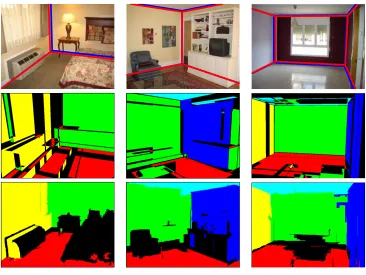
Figure 3: The top row shows three indoor scenes from the layout dataset (Hedau et al., 2009). Orientation maps (Lee et al., 2009) and geometric context (Hoiem et al., 2007) features for the respective images are illustrated in the center and bottom row respectively.

Note that the log-beliefs are balanced by cr, to compensate for their exponent peaked-ness. This balancing makes the objective well defined at cr = 0 as the limit of cr → 0. In this case the program is non-smooth and one needs to consider the sub gradient in the form of max-beliefs. However, this setting was already developed, although in the different context of structured-SVMs using dual losses, and we refer the interested reader to Meshi et al. (2010) for more details.

6. Experiments

vp₀

vp₁ vp₂ y1

y2

y3 y4

r1

r2

r3 r4

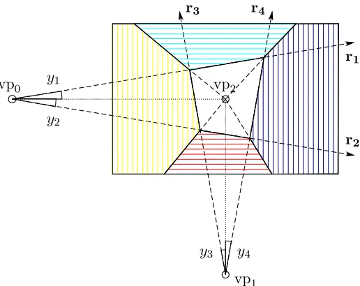
Figure 4: Ray parameterization of the layout given detected vanishing points. A state of a discretized variableyi gives rise to a particular rayrioriginating from a detected

vanishing point. Four rays are sufficient to define a room layout, i.e., the location of the walls.

In the following we demonstrate the various properties of blending learning and inference. For this purpose we elaborate more carefully on a 3D scene understanding application (Schwing et al., 2012a) evaluated on the well known layout dataset (Hedau et al., 2009) containing 314 indoor images. Given a single image similar to the ones illustrated in the top row of Figure 3, we aim at estimating the location of the left, front and right walls as well as ceiling and floor. Formulating this task as a pixelwise semantic segmentation application permits a large number of configurations that are physically not plausible. We therefore constrain the space of configurations by parametrizing the application using three dominant vanishing points as illustrated in Figure 4. The random variables y1, . . . , y4 correspond to discretized angles of rays, each one originating from a detected vanishing point. Such a parametrization in terms of rays permits only physically plausible configurations and assumes the world to be Manhattan like, i.e., the observed room is aligned according to the three dominant directions.

To obtain the dominant directions we employ the vanishing point detector of Hedau et al. (2009). Due to the involved randomness it failed in our case on 9 training images and was successful on all 105 test set instances. For imagex and a given layout hypothesis y = (y1, . . . , y4) we compute a 55-dimensional feature vector φ(x, y) which is constructed based on geometric context (Hoiem et al., 2007) and orientation maps (Lee et al., 2009) illustrated in the middle and bottom row of Figure 3 respectively.

Figure 5: Left: Test set percentage pixel error on the layout data set Hedau et al. (2009). Right: Test set pixel classification error in % on the bedroom data set of Hedau et al. (2010).

feature vector. Similarly for orientation map evidence we count how many of the five possible labels fell onto each of the five hypothesized wall areas, resulting in a 5·5 = 25 dimensional vector. Combining both image evidences we hence obtain a feature vector φ having a total ofK= 55 entries, each being represented by a graphical model having nodes Rk,k∈ {1, . . . , K}.

Note that a vanilla implementation of these color counting features results in potentials of order four for the front wall, and of order three for all other walls. High-order potentials increase the complexity of learning and inference, therefore, the exact decomposition of those high-order potentials into pairwise terms using ‘integral geometry’ Schwing et al. (2012a) is important for tractability.

In our experiments we learn and infer with the same counting numbers. For example, when we learn log-beliefs by setting the counting numbers to 1, we also infer with log-beliefs at test time, namely setting the counting numbers to 1. Figure 5 demonstrates the tradeoffs of learning with various counting numbers. This experiment also compares to blending of structured-SVMs of Meshi et al. (2010) when setting the counting numbers to 0.

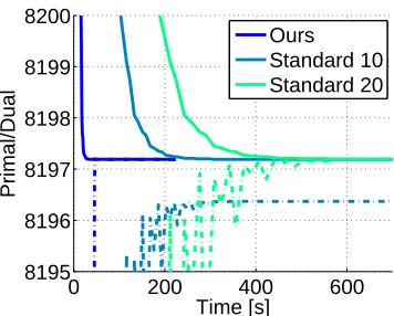
In Figure 6 we illustrate the optimized cost function, i.e., the surrogate training loss over wall clock time. We observe that our discussed blended learning approach (‘Ours’) converges quickly, i.e., in less than 50 seconds, to a zero primal dual gap. In contrast it takes the standard learning approach (‘Standard 20’), which performs 20 message passing iterations, more than 600 seconds to converge to the same solution. Hence blended learning is more than 10 times faster on this example. Next we investigate whether a standard message passing approach with 20 iterations is overly pessimistic for this dataset. To this end we use 10 message passing iterations and refer to the obtained result as ‘Standard 10.’ Investigating Figure 6 more carefully we observe that 10 message passing iterations are not sufficient to close the duality gap, i.e., the approach does never converge to the same solution.

0 200 400 600 8195

8196 8197 8198 8199 8200

Time [s]

Primal/Dual

Ours Standard 10 Standard 20

Figure 6: Primal surrogate loss (dashed) and its dual (solid) over wall clock time measured in seconds for blended learning, the standard approach with 10 iterations, and the standard approach with 20 iterations.

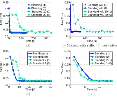
(2010), the test set performance of convex learning with 20 message passing iterations with both counting numbers equal to zero (cf. Meshi et al. (2010)) and one, i.e., ‘Standard 20 (0)’ and ‘Standard 20 (1)’ respectively. We observe that the test set accuracy drops significantly faster which is expected since we are able to update the parameter vector more frequently. Similar to the aforementioned surrogate training loss result we observe a performance im-provement of more than one order of magnitude, i.e., we obtain accurate test set results more than 10 times faster.

In a next experiment we evaluate the importance of the loss function. The results are illustrated in Figure 7(b). We observe the loss to be important for the case where the counting numbers equal zero. We are able to obtain a performance similar to loss-included setting if the counting numbers are equal to one. However algorithms which do not use a loss function while having counting numbers equal to zero got stuck prematurely and are hence not even visible in Figure 7(b), where the scale was adjusted to fit the other plots.

Next we observe the behavior if we reduce the number of iterations for standard learning from 20 down to 2. Recall, from the surrogate training loss results that the primal-dual gap will not reach zero in this setting. The test set errors are illustrated in Figure 7(c). We observe that the standard method is approaching the blending technique. This indicates that a primal-dual gap is not necessarily important for good generalization performance.

0 100 200 300 0.1

0.15 0.2 0.25 0.3 0.35

Test Error

Time [s]

Blending (1) Blending (0) Standard 20 (1) Standard 20 (0)

0 200 400

0.1 0.15 0.2 0.25 0.3 0.35

Test Error

Time [s]

Blending w/L (1) Blending w/L (0) Standard w/L 20 (1) Standard w/L 20 (0)

(a) (b) Methods with suffix ‘(0)’ not visible.

0 10 20 30 40

0.1 0.15 0.2 0.25 0.3 0.35

Test Error

Time [s]

Blending (1) Blending (0) Standard 2 (1) Standard 2 (0)

0 5 10

0.1 0.15 0.2 0.25 0.3 0.35

Test Error

Time [s]

Blending (1) Blending (0) Blending 2 (1) Blending 2 (0)

(c) (d)

Figure 7: A comparison of the test set error over training time for different parameter set-tings. In (a) we compare standard learning with blended learning when including a loss function. In (b) we provide the comparison when not using a loss function. Note that using MAP estimation without loss got stuck at a high error. The re-sults in (c) demonstrate the effects when reducing the iterations of the standard learning method, while (d) illustrates the flexibility offered by blending where we use two message passing iterations before updating the parameters.

7. Conclusion and Discussion

This work extends Hazan and Urtasun (2010) while simplifying its theoretical and practical concepts. Specifically, we introduce the learning program as maximizing log-beliefs, explain the relations between nested and blended learning-inference and derives a blending algo-rithm for general graphs. This work is extended to latent variables (Schwing et al. (2012b)) and deep learning (Chen∗ et al. (2015); Schwing and Urtasun (2015)). The effectiveness of the discussed framework was recently illustrated by employing this algorithm as the learn-ing engine for various computer vision tasks: 2D scene understandlearn-ing (Yao et al. (2012)), 3D scene understanding (Lin et al. (2013)), shape reconstruction (Salzmann and Urtasun (2012)) indoor scene understanding (Schwing et al. (2012a); Schwing and Urtasun (2012)), depth estimation (Yamaguchi et al. (2012)), flow estimation (Yamaguchi et al. (2013)) and visual-language understanding (Fidler et al. (2013)). We believe it is interesting to show in the future if this algorithm provides state-of-the-art performance in domains other than computer vision, or whether the statistics in computer vision are used by this approach in a special manner.

The computational complexity of our algorithm depends on norm-products over the labels of regions. Therefore, efficient techniques over large regions in inference can be applied as sub-procedure in our algorithm, e.g., Kohli et al. (2009); Batra et al. (2010); Tarlow et al. (2010, 2011); Tarlow and Zemel (2012).

In our framework, we can enforce the moment matching constraints through general concave functions. These function translate to a regularization in the primal. For compu-tational efficiency we choose the square function but we did not investigate the different moment matching and regularization functions. Moreover, we enforce the marginalization constraints through indicator functions, in order to obtain closed-form solution in the pri-mal block coordinate descent. However, we have shown that using the penalty method we can enforce the marginalization constraints with different convex functions. Further ex-plorations of structured prediction with squared penalties appears in work by Meshi et al. (2015). We leave the affect of general convex functions on moment matching and regu-larization, as well as marginalization constraints and efficient message-passing to future research.

Interestingly, our approach confirms that the parameters of graph based structured predictors can be efficiently learned in many real-life problems. This validates the intuition behind the theoretical results of Wainwright et al. (2003); Wainwright (2006) which asserts that whenever learning and inference occur together one can use pseudo moment matching for learning the parameters. This concept was put forward in the general framework of learning to reason by Khardon and Roth (1997) and we leave for future research to find different frameworks which have similar learning-prediction robustness.

8. Extensions: regularizations and the penalty method

Duality theory turned out to be very effective in machine learning as it provides a principled way to decompose the different ingredients of the primal objective through its Lagrange multipliers. The dual decomposition in turn provides the means to efficiently estimate the different ingredients while maintaining their consistency using the dual objective.

the primal program using extended real-valued convex functions, which are functions that can take on the value of infinity. By using extended real-valued functions we can ignore their domains, i.e., points for which a function attains the value other than infinity, thus simplifying the derivations. The dual programs of extended real valued convex functions g(µ) are conveniently formulated in terms of their conjugate dual

g∗(z) = max µ

n

µ>z−g(µ)

o

.

Throughout this work we use the following duality theorem, known as the Fenchel duality (cf. Fenchel (1951); Rockafellar (1970); Bertsekas et al. (2003)):

Theorem 6 Letf(·), h1(·), h2(·) be extended real-valued, continuous and convex functions. The following are primal and dual programs:

min λ,w

X

(x,y)∈S,r∈R

f

θr(·;x, w, λ) +`r(·, yr)

+X k

h1(wk) +

X

(x,y),r,yˆr,p∈P(r)

h2(λr→p(ˆyr;x))

max br

X

(x,y)∈S,r∈R

−f∗(br) +

X

ˆ yr

br(ˆyr|x)`r(yr,yˆr)

−X k

h∗₁

_X

(x,y),r

X

ˆ yr

br(ˆyr)φk,r(x,yˆr)−φk,r(x, yr)

− X

(x,y),r,yˆr,p

h∗₂ X ˆ yp\yˆr

bp(ˆyp|x)−br(ˆyr|x)

Proof The proof goes along the lines of Theorem 5. The dual program takes the form

X

(x,y)∈S,r∈R

−f∗(br) +

X

ˆ yr

br(ˆyr|x)`r(yr,yˆr)

−X k

h∗₁(uk)−

X

(x,y),r,yˆr,p

h∗₂(δr→p(ˆyr;x))

s.t. uk=

X

(x,y),r

X

ˆ yr

br(ˆyr|z)φk,r(x,yˆr)−φk,r(x, yr)

δr→p(ˆyr;x) =

X

ˆ yp\yˆr

bp(ˆyp|x)−br(ˆyr|x)

Constructing its Lagrangian with the Lagrange multipliers wk, λr→p(ˆyr;x), we obtain the primal programp(w, λ) = maxb,u,dL(br, λ, w) which decomposes toP(x,y),rmaxbr{−f

∗_(b

r)+

P

ˆ

yrbr(yr|x)(`r(yr,yˆr)+θr(ˆyr;x, w, λ))}+

P

(x,y),r,yˆr,pmaxδ{δr→p(ˆyr)λr→p(ˆyr)−h

∗

2(δr→p(ˆyr))}+ w>e+P

kmaxuk{wkuk−h

∗

1(uk)}, where ek =P(x,y),rφk,r(x, yr). The result then follows since the conjugate dual off∗(), h∗₁(), h∗₂() are f(), h1(), h2() respectively.

The primal program translates the dual penalty functions h∗₁(·), h∗

2(·) to regularization functionsh1(·),h2(·). Whenever the primal functions are smooth we can use the chain rule to derive the primal program gradients:

∂ ∂wk

: X

(x,y)∈S

X

r∈R

X

ˆ yr

∂f(θr(·;z, w, λ)) ∂θr(ˆyr;z, w, λ)

φk,r(x,yˆr)−φk,r(x, yr)

+∇h_k(wk)

∂ ∂λr→p(ˆyr;x)

: X

ˆ yp\ˆyr

∂f(θp(·;z, w, λ)) ∂θp(ˆyp;z, w, λ)

−∂f(θr(·;z, w, λ)) ∂θr(ˆyr;z, w, λ)

+∇h2(λr→p(ˆyr;x))

The above generalizes the learning-inference blending algorithm for general functions f(·) and regularizationsh1(·), h2(·). The power of setting f(·) to be the log-partition func-tion is that its derivatives are beliefs therefore we obtain an intuitive probabilistic interpre-tations. The parameters derivatives result in moment matching constraints

X

(x,y)∈S

X

r∈R

X

ˆ yr

∂f(θr(·;z, w, λ)) ∂θr(ˆyr;z, w, λ)

φk,r(x,yˆr)−φk,r(x, yr)

.

The re-parametrization derivatives with respect to the messagesλr→p(yr;x) are then marginal-ization constraints

X

ˆ yp\yˆr

∂f(θp(·;z, w, λ)) ∂θp(ˆyp;z, w, λ)

−∂f(θr(·;z, w, λ)) ∂θr(ˆyr;z, w, λ)

Moreover, wheneverh2(·)≡0, we are able to derive closed-form update rules.

Acknowledgments

We are most grateful to David McAllester for helpful discussions, and the anonymous re-viewers for their helpful comments. This work was supported in part by the German-Israeli Foundation grant I-1123-407.6-2013.

References

S. M. Aji and R. J. McEliece. The generalized distributive law and free energy minimization.

In Allerton, 2001.

D. Anguelov, B. Taskar, V. Chatalbashev, D. Koller, D. Gupta, G. Heitz, and A.Y. Ng. Discriminative learning of markov random fields for segmentation of 3D range data. In

Proc. CVPR, 2005.

D. Batra, A. C. Gallagher, D. Parikh, and T. Chen. Beyond trees: MRF inference via outer-planar decomposition. In Proc. CVPR, 2010.

D. P. Bertsekas, A. Nedi´c, and A. E. Ozdaglar. Convex Analysis and Optimization. Athena Scientific, 2003.

M. Collins. Discriminative training methods for hidden markov models: Theory and exper-iments with perceptron algorithms. In Proc. ACL, 2002.

J. Domke. Parameter learning with truncated message-passing. In Proc. CVPR, 2011.

P. Felzenszwalb, R. Girshick, D. McAllester, and D. Ramanan. Object detection with discriminatively trained part based models. PAMI, 2010.

W. Fenchel. Convex cones, sets, and functions. Princeton University, Department of Math-ematics, 1951.

S. Fidler, A. Sharma, and R. Urtasun. A sentence is worth a thousand pixels. In Proc. CVPR, 2013.

T. Hazan and A. Shashua. Convergent message-passing algorithms for inference over general graphs with convex free energies. In Proc. UAI, 2008.

T. Hazan and A. Shashua. Norm-product belief propagation: Primal-dual message-passing for approximate inference. Information Theory, 2010.

T. Hazan and R. Urtasun. A Primal-Dual Message-Passing Algorithm for Approximated Large Scale Structured Prediction. In Proc. NIPS, 2010.

V. Hedau, D. Hoiem, and D. Forsyth. Recovering the Spatial Layout of Cluttered Rooms.

In Proc. ICCV, 2009.

Varsha Hedau, Derek Hoiem, and David Forsyth. Thinking Inside the Box: Using Appear-ance Models and Context Based on Room Geometry. In Proc. ECCV, 2010.

T. Heskes. Convexity arguments for efficient minimization of the Bethe and Kikuchi free energies. Journal of Artificial Intelligence Research, 2006.

D. Hoiem, A. A. Efros, and M. Hebert. Recovering Surface Layout from an Image. IJCV, 2007.

R. Khardon and D. Roth. Learning to reason. Journal of the ACM (JACM), 1997.

P. Kohli, L. Ladick`y, and P. H. S. Torr. Robust higher order potentials for enforcing label consistency. IJCV, 2009.

T. Koo, A. M. Rush, M. Collins, T. Jaakkola, and D. Sontag. Dual decomposition for parsing with non-projective head automata. InProc. EMNLP, 2010.

J. Lafferty, A. McCallum, and F. Pereira. Conditional random fields: Probabilistic models for segmenting and labeling sequence data. In Proc. ICML, 2001.

S. L. Lauritzen. Graphical models, volume 17. Oxford University Press, USA, 1996.

G. Lebanon and J. Lafferty. Boosting and maximum likelihood for exponential models.

D. C. Lee, M. Hebert, and T. Kanade. Geometric Reasoning for Single Image Structure Recovery. InProc. CVPR, 2009.

A. Levin and Y. Weiss. Learning to Combine Bottom-Up and Top-Down Segmentation.

In Proc. ECCV, 2006.

D. Lin, S. Fidler, and R. Urtasun. Holistic scene understanding for 3d object detection with rgbd cameras. In Proc. ICCV, 2013.

T. Meltzer, A. Globerson, and Y. Weiss. Convergent message passing algorithms-a unifying view. In Proc. UAI, 2009.

O. Meshi, A. Jaimovich, A. Globerson, and N. Friedman. Convexifying the bethe free energy. In Proc. UAI, 2009.

O. Meshi, D. A. Sontag, T. S. Jaakkola, and A. Globerson. Learning efficiently with ap-proximate inference via dual losses. In Proc. ICML, 2010.

O. Meshi, N. Srebro, and T. Hazan. Efficient Training of Structured SVMs via Soft Con-straints. In Proc. AISTATS, 2015.

Y. Nesterov. Introductory lectures on convex optimization: A basic course. Springer, 2004.

R.T. Rockafellar. Convex analysis. Princeton university press, 1970.

M. Salzmann and R. Urtasun. Beyond Feature Points: Structured Prediction for Monocular Non-rigid 3D Reconstruction. In Proc. ECCV, 2012.

A. G. Schwing and R. Urtasun. Efficient exact inference for 3d indoor scene understanding.

In Proc. ECCV, 2012.

A. G. Schwing and R. Urtasun. Fully Connected Deep Structured Networks. http://arxiv.org/abs/1503.02351, 2015.

A. G. Schwing, T. Hazan, M. Pollefeys, and R. Urtasun. Distributed message passing for large scale graphical models. InProc. CVPR, 2011.

A. G. Schwing, T. Hazan, M. Pollefeys, and R. Urtasun. Efficient structured prediction for 3d indoor scene understanding. In Proc. CVPR, 2012a.

A. G. Schwing, T. Hazan, M. Pollefeys, and R. Urtasun. Efficient Structured Prediction with Latent Variables for General Graphical Models. In Proc. ICML, 2012b.

D. Sontag, T. Meltzer, A. Globerson, T. Jaakkola, and Y. Weiss. Tightening LP relaxations for MAP using message passing. In Proc. UAI, 2008.

C. Sutton and A. McCallum. Piecewise training for structured prediction. Machine Learn-ing, 2009.

D. Tarlow and R. S. Zemel. Structured output learning with high order loss functions. In

Proc. AISTATS, 2012.

D. Tarlow, I. E. Givoni, and R. S. Zemel. Hopmap: Efficient message passing with high order potentials. In Proc. AISTATS, 2010.

D. Tarlow, D. Batra, P. Kohli, and V. Kolmogorov. Dynamic tree block coordinate ascent.

Proc. ICML, 2011.

B. Taskar, C. Guestrin, and D. Koller. Max-margin Markov networks. Proc. NIPS, 2004.

B. Taskar, V. Chatalbashev, D. Koller, and C. Guestrin. Learning structured prediction models: A large margin approach. InProc. ICML, 2005.

P. Tseng and D.P. Bertsekas. Relaxation methods for problems with strictly convex sepa-rable costs and linear constraints. Mathematical Programming, 38(3):303–321, 1987.

I. Tsochantaridis, T. Hofmann, T. Joachims, and Y. Altun. Support vector machine learning for interdependent and structured output spaces. InProc. ICML, 2004.

M. J. Wainwright. Estimating the Wrong Graphical Model: Benefits in the Computation-Limited Setting. JMLR, 2006.

M. J. Wainwright and M. I. Jordan. Graphical models, exponential families, and variational inference. Foundations and TrendsR in Machine Learning, 2008.

M. J. Wainwright, T. S. Jaakkola, and A. S. Willsky. Tree-reweighted belief propaga-tion algorithms and approximate ML estimapropaga-tion by pseudo-moment matching. In Proc.

Workshop on AI and Stats., 2003.

M. J. Wainwright, T. S. Jaakkola, and A. S. Willsky. A new class of upper bounds on the log partition function. Trans. on Information Theory, 51(7):2313–2335, 2005.

K. Yamaguchi, T. Hazan, D. McAllester, and R. Urtasun. Continuous markov random fields for robust stereo estimation. In Proc. ECCV, 2012.

K. Yamaguchi, D. McAllester, and R. Urtasun. Robust monocular epipolar flow estimation.

In Proc. CVPR, 2013.

C. Yanover, O. Schueler-Furman, and Y. Weiss. Minimizing and learning energy functions for side-chain prediction. In RECOMB. Springer, 2007.

J. Yao, S. Fidler, and R. Urtasun. Describing the scene as a whole: Joint object detection, scene classification and semantic segmentation. In Proc. CVPR, 2012.