Variational Dependent Multi-output Gaussian Process
Dynamical Systems
Jing Zhao ∗ [email protected]
Shiliang Sun ∗ [email protected]
Department of Computer Science and Technology East China Normal University
500 Dongchuan Road, Shanghai 200241, P. R. China
Editor:Neil Lawrence
Abstract
This paper presents a dependent multi-output Gaussian process (GP) for modeling complex dynamical systems. The outputs are dependent in this model, which is largely different from previous GP dynamical systems. We adopt convolved multi-output GPs to model the outputs, which are provided with a flexible multi-output covariance function. We adapt the variational inference method with inducing points for learning the model. Conjugate gradient based optimization is used to solve parameters involved by maximizing the vari-ational lower bound of the marginal likelihood. The proposed model has superiority on modeling dynamical systems under the more reasonable assumption and the fully Bayesian learning framework. Further, it can be flexibly extended to handle regression problems. We evaluate the model on both synthetic and real-world data including motion capture data, traffic flow data and robot inverse dynamics data. Various evaluation methods are taken on the experiments to demonstrate the effectiveness of our model, and encouraging results are observed.
Keywords: Gaussian process, variational inference, dynamical system, multi-output modeling
1. Introduction
Dynamical systems are widespread in the research area of machine learning. Multi-output time series such as motion capture data, traffic flow data and video sequences are typical examples generated from these systems. Data generated from these dynamical systems usually have the following characteristics. 1) Implicit dynamics exist in the data, and the relationship between the observations and the time indices is nonlinear. For example, the transformation of the frames of a video over time is complex. 2) Possible dependency exists among multiple outputs. For example, for motion capture data, the position of the hand is often closely related to the position of the arm. A simple and straightforward method to model this kind of dynamical systems is to use Gaussian processes (GPs), since GPs provide an elegant method for modeling nonlinear mappings in the Bayesian nonparametric learning framework (Rasmussen and Williams, 2006). Some extensions of GPs have been developed in recent years to better model the dynamical systems. The dynamical systems
modeled by GPs are called the Gaussian process dynamical systems (GPDSs). However, the existing GPDSs have a limitation of ignoring the dependency among the multiple outputs, that is, they may not make full use of the characteristics of data. Our work aims to model the complex dynamical systems more reasonably and flexibly.
Gaussian process dynamical models (GPDMs) as extensions of the GP latent variable model (GP-LVM) (Lawrence, 2004, 2005) were proposed to model human motion (Wang et al., 2006, 2008). The GP-LVM is a nonlinear extension of the probabilistic principal component analysis (Tipping and Bishop, 1999) and is a probabilistic model where the out-puts are observed while the inout-puts are hidden. It introduces latent variables and performs a nonlinear mapping from the latent space to the observation space. The GP-LVM pro-vides an unsupervised non-linear dimensionality reduction method by optimizing the latent variables with the maximum a posteriori (MAP) solution. The GPDM allows to model nonlinear dynamical systems by adding a Markov dynamical prior on the latent space in the GP-LVM. It captures the variability of outputs by constructing the variance of outputs with different parameters. Some research of adapting GPDMs to specific applications was developed, such as object tracking (Urtasun et al., 2006), activity recognition (Gamage et al., 2011) and synthesis, and computer animation (Henter et al., 2012).
Similarly, Damianou et al. (2011, 2014) extended the GP-LVM by imposing a dynamical prior on the latent space to the variational GP dynamical system (VGPDS). The nonlinear mapping from the latent space to the observation space in the VGPDS allows the model to capture the structures and characteristics of data in a relatively low dimensional space. Instead of seeking a MAP solution for the latent variables as in GPDMs, VGPDSs used a variational method for model training. This follows the variational Bayesian method for training the GP-LVM (Titsias and Lawrence, 2010), in which a lower bound of the logarith-mic marginal likelihood is computed by variationally integrating out the latent variables that appear nonlinearly in the inverse kernel matrix of the model. The variational Bayesian method was built on the method of variational inference with inducing points (Titsias, 2009). The VGPDS approximately marginalizes out the latent variables and leads to a rigorous lower bound on the logarithmic marginal likelihood. The model and variational parame-ters of the VGPDS can be learned through maximizing the variational lower bound. This variational method with inducing points was also employed to integrate out the warping functions in the warped GP (Snelson et al., 2003; L´azaro-gredilla, 2012). Park et al. (2012) developed an almost direct application of VGPDSs to phoneme classification, in which a variance constraint in the VGPDS was introduced to eliminate the sparse approximation error in the kernel matrix. Besides variational approaches, expectation propagation based methods (Deisenroth and Mohamed, 2012) are also capable of conducting approximate in-ference in GPDSs.
series of extensions of LFMs were presented such as linear, nonlinear, cascaded and switch-ing dynamical LFMs ( ´Alvarez et al., 2011, 2013). In addition, sequential inference methods for LFMs have also been developed (Hartikainen and S¨arkk¨a, 2012). ´Alvarez and Lawrence (2011) employed convolution processes to account for the correlations among outputs to construct a convolved multiple outputs GP (CMOGP) which can be regarded as a specific case of LFMs. To overcome the difficulty of time and storage complexities for large data sets, some efficient approximations for the CMOGP were constructed through the convo-lution formalism ( ´Alvarez et al., 2010; ´Alvarez and Lawrence, 2011). This leads to a form of covariance similar in spirit to the so called deterministic training conditional (DTC) approximation (Csat´o and Opper, 2001), fully independent training conditional (FITC) ap-proximation (Qui˜nonero-Candela and Rasmussen, 2005; Snelson and Ghahramani, 2006) and partially independent training conditional (PITC) approximation (Qui˜nonero-Candela and Rasmussen, 2005) for a single output (Lawrence, 2007). The CMOGP is then enhanced and extended to the collaborative multi-output Gaussian process (COGP) for handling large scale cases (Nguyen and Bonilla, 2014). Besides CMOGPs, Wilson et al. (2012) combined neural networks with GPs to construct a GP regression network (GPRN). Outputs in the GPRN are linear combinations of the shared adaptive latent basis functions with input de-pendent weights. However, these two models are neither introduced nor directly suitable for complex dynamical system modeling. When a dynamical prior is imposed, marginalizing over the latent variables is needed, which can be very challenging.
In this paper, we propose a variational dependent multi-output GP dynamical system (VDM-GPDS). It is a hierarchical Gaussian process model in which the dependency among all the observations is well captured. Specifically, the convolved process covariance function ( ´Alvarez and Lawrence, 2011) is employed to capture the dependency among all the data points across all the outputs. To learn the VDM-GPDS, we first approximate the latent functions in the convolution processes, and then variationally marginalize out the latent variables in the model. This leads to a convenient lower bound of the logarithmic marginal likelihood, which is then maximized by the scaled conjugate gradient method to find out the optimal parameters.
An earlier short version of this work appeared in Zhao and Sun (2014). In this paper, we add detailed derivations of the variational inference and provide the gradients of the objective function with respect to the parameters. Moreover, we analyze the performance and efficiency of the proposed model. In addition, we supplement experiments on real-world data and all the experimental results are measured under various evaluation criteria.
The rest of the paper is organized as follows. First, we give the model for nonlinear dynamical systems in Section 2, where we use convolution process covariance functions to construct the covariance matrix of the dependent multi-output latent variables. Section 3 gives the derivation of the variational lower bound of the marginal likelihood function and optimization methods. Prediction formulations are introduced in Section 4. Related work is analyzed and compared in Section 5. Experimental results are reported in Section 6 and finally conclusions are presented in Section 7.
2. The Proposed Model
Suppose we have multi-output time series data {yn, tn}nN=1, where yn ∈RD is an observa-tion at timetn∈R+. We assume that there are low dimensional latent variables that govern the generation of the observations and a GP prior for the latent variables conditional on time captures the dynamical driving force of the observations, as in Damianou et al. (2011). However, a large difference compared with their work is that we explicitly model the de-pendency among the outputs through convolution processes ( ´Alvarez and Lawrence, 2011).
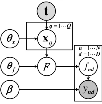
Our model is a four-layer GP dynamical system. Here t ∈ RN represents the input variables in the first layer. The matrix X ∈ RN×Q represents the low dimensional latent variables in the second layer with element xnq =xq(tn). Similarly, the matrix F ∈RN×D denotes the latent variables in the third layer, with element fnd =fd(xn) and the matrix
Y ∈ RN×D denotes the observations in the fourth layer whose nth row corresponds to
yn. The model is composed of an independent multi-output GP mapping from t to X, a dependent multi-output GP mapping fromX toF, and a linear mapping from F toY.
Specifically, for the first mapping, x is assumed to be a multi-output GP indexed by timet similarly to Damianou et al. (2011), that is
xq(t) ∼ GP(0, κx(t, t0)), q = 1, ..., Q, (1)
functions take the following forms.
κx(RBF)(ti, tj) =σ2rbfe
(ti−tj)2 2`2 ,
κx(M atern´ 3/2)(ti, tj) =σ2mat(1 + √
3|ti−tj|
` )e
−√3|ti−tj|
` ,
κx(RBF periodic)(ti, tj) =σ2pere
−1 2
sin2( 2Tπ(ti−tj))
` .
(2)
According to the conditional independency assumption among the latent variables{xq}Qq=1, we have
p(X|t) = Q
Y
q=1
p(xq|t) = Q
Y
q=1
N(xq|0,Kt,t), (3)
whereKt,t is the covariance matrix constructed byκx(t, t0).
For the second mapping, we assume that f is another multi-output GP indexed by x, whose outputs are dependent, that is
fd(x)∼ GP(0, κfd,fd0(x,x
0)), d, d0= 1, ..., D, (4)
where κfd,fd0(x,x
0) is a convolved process covariance function. The convolved process
co-variance function captures the dependency among all the data points across all the outputs with parameters θf = {{Λk},{Pd},{Sd,k}}. The detailed formulation of this covariance function will be given in Section 2.1. From the conditional dependency among the latent variables {fnd}N,Dn=1,d=1, we have
p(F|X) =p(f|X) =N(f|0,Kf,f), (5)
wheref is a shorthand for [f1>, ...,fD>]> and Kf,f sizedN D×N D is the covariance matrix
in which the elements are calculated by the covariance function κfd,fd0(x,x
0).
The third mapping, which is from the latent variable fnd to the observationynd, can be written as
ynd=fnd+nd, nd∼ N(0, β−1). (6)
Since the observations{ynd}N,Dn=1,d=1 are conditionally independent on F, we get
p(Y|F) = D
Y
d=1
N
Y
n=1
N(ynd|fnd, β−1). (7)
Given the above setting, the graphical model for the proposed VDM-GPDS on the training data {yn, tn}Nn=1 can be depicted as Figure 1. From (3), (5) and (7), the joint
probability distribution for the VDM-GPDS model is given by
p(Y, F, X|t) =p(Y|F)p(F|X)p(X|t) =p(f|X) D
Y
d=1
N
Y
n=1
p(ynd|fnd) Q
Y
q=1
t
q
x
1"
q Q
y
nd1"
n N
E
x
T
f
nd(
1"
d D
f
T
Figure 1: The graphical model for VDM-GPDS.
2.1 Convolved Process Covariance Function
Since the outputs in our model are dependent, we need to capture the correlations among all the data points across all the outputs. Bonilla et al. (2007) and Luttinen and Ilin (2012) used a Kronecker product covariance matrix with the form ofKF F =KDD⊗KN N, whereKDD is the covariance matrix among the output dimensions, and KN N is the covariance matrix calculated solely from the data inputs. This Kronecker form kernel is constructed from the processes which involve some form of instantaneous mixing of a series of independent processes. This is very limited and actually a special case of some general covariances when covariances calculated from outputs and inputs are independent ( ´Alvarez et al., 2012). For example, if we want to model two output processes in such a way that one process was a blurred version of the other, we cannot achieve this through the instantaneous mixing ( ´Alvarez and Lawrence, 2011). In this paper, we use a more general and flexible kernel in which KDD and KN N are not separated. In particular, the convolution processes ( ´Alvarez and Lawrence, 2011) are employed to model the latent function F(X).
Now we introduce how to construct the convolved process covariance functions. By using independent latent functions {uk(x)}Kk=1 and smoothing kernels {Gd,k(x)}D,Kd=1,k=1 in the
convolution processes, each latent function in (4) in the VDM-GPDS is expressed through a convolution integral,
fd(x) = K
X
k=1 Z
X
Gd,k(x−x˜)uk(˜x)d˜x. (9)
The most common construction is to use Gaussian forms for{uk(x)}Kk=1and{Gd,k(x)}D,Kd=1,k=1. So the smoothing kernel is assumed to be
Gd,k(x) =Sd,kN(x|0, Pd), (10)
Gaussian with covariance function
κk x,x0
=N x−x0|0,Λk. (11)
Thus, the covariance betweenfd(x) and fd0(x0) is
κfd,fd0(x,x
0) =
K
X
k=1
Sd,kSd0,kN(x|x0, Pd+Pd0 + Λk). (12)
The covariance betweenfd(x) anduk(x0) is
κfd,uk(x,x
0) =S
d,kN x−x0|0, Pd+ Λk
. (13)
These covariance functions (11), (12) and (13) will later be used for approximate in-ference in Section 3. Compared with Kronecker form kernels, our used convolved kernels have the following advantages. From the perspective of constructing the process fd, con-volved kernels are constructed using the convolution process fd in which the smoothing kernelsGd,k(x) related toxare employed while Kronecker form kernels are constructed us-ingfd(x) =aduk(x) in whichadhas no relation tox ( ´Alvarez and Lawrence, 2011). From the perspective of kernels, for different dimensions d and d0, convolved kernels allow that the covariances {κfd,fd0(x,x
0)} are related to different terms N(x|x0, P
d+Pd0+ Λk) while
Kronecker form kernels indicate that different covariances {κfd,fd0(x,x
0)} share the same
termκq(x,x0). Thus, our used convolved kernels are more general. 3. Inference and Optimization
As described above, the proposed VDM-GPDS explicitly models the dependency among multiple outputs, which makes it largely distinct to the previous VGPDS and other GP dynamical systems. In order to make it easy to implement by extending the existing frame-work of the VGPDS, in the current and the following sections, we will deduce the variational lower bound for the logarithmic marginal likelihood and the posterior distribution for pre-diction in a formulation similar to the VGPDS. However, many details as described in the paper are specific to our model, and some calculations are more involved.
The fully Bayesian learning for our model requires maximizing the logarithm of the marginal likelihood (Bishop, 2006)
p(Y|t) =
Z
p(Y|F)p(F|X)p(X|t)dXdF. (14)
Note that the integration w.r.t X is intractable, because X appears nonlinearly in the inverse of the matrixKf,f. We attempt to make some approximations for (14).
To begin with, we approximate p(F|X) which is constructed by convolution process
E(uk(˜x)|uk). Let U ={uk}Kk=1 and u = [u>1, ...,u>K]>. The probability distribution of u can be expressed as
p(u|Z) =N(0,Ku,u), (15)
whereKu,u is constructed byκk(x,x0) in (11). Combining (9) and (15), we get the proba-bility distribution of f conditional onu, X, Z as
p(f|u, X, Z) =N(f|Kf,uK−1u,uu,Kf,f −Kf,uK−1u,uKu,f), (16)
whereKf,uis the cross-covariance matrix betweenfd(x) anduk(z) with elementκfd,uk(x,x
0)
in (13), the block-diagonal matrix Ku,u is the covariance matrix between uk(z) and uk(z0) with elementκk(x,x0) in (11), andKf,f is the covariance matrix betweenfd(x) andfd0(x0)
with element κfd,fd0(x,x
0) in (12). Therefore, p(F|X) is approximated by
p(F|X)≈p(f|X, Z) =
Z
p(f|u, X, Z)p(u|Z)du, (17) and p(Y|t) is converted to
p(Y|t)≈p(Y|t, Z) =
Z
p(y|f)p(f|u, X, Z)p(u|Z)p(X|t)dF dU dX, (18)
where p(u|Z) = N(0,Ku,u) and y = [y1>, ...,yD>]
>. It is worth noting that the marginal
likelihood in (18) is still intractable as the integration with respect to X remains difficult. Then, we introduce a lower bound of the logarithmic marginal likelihood logp(Y|t) using variational methods. We construct a variational distributionq(F, U, X|Z) to approx-imate the posterior distribution p(F, U, X|Y,t) and compute the Jensen’s lower bound on logp(Y|t) as
L=
Z
q(F, U, X|Z) logp(Y, F, U, X|t, Z)
q(F, U, X|Z) dXdU dF. (19)
The variational distribution is assumed to be factorized as
q(F, U, X|Z) =p(f|u, X, Z)q(u)q(X). (20) The distributionp(f|u, X, Z) in (20) is the same as the second term in (18), which will be eliminated in the term logp(qY,F,U,X(F,U,X||tZ,Z) ) in (19). The distributionq(u) is an approximation to the posterior distributionp(u|X, Y), which is arguably Gaussian by maximizing the vari-ational lower bound (Titsias and Lawrence, 2010; Damianou et al., 2011). The distribution
q(X) is an approximation to the posterior distribution p(X|Y), which is assumed to be a product of independent Gaussian distributions q(X) =QQ
q=1N(xq|µq, Sq).
After some calculations and simplifications, the lower bound withX,U andF integrated out becomes
L= log
"
βN D2 |Ku,u| 1 2
(2π)N D2 |βψ2+Ku,u| 1 2
exp{−1 2y
>Wy} #
−βψ0
2 +
β
2Tr(K
−1
u,uψ2)−KL[q(X)||p(X|t)],
where W =βI −β2ψ1(βψ2+Ku,u)−1ψ>1, ψ0 = Tr(hKf,fiq(X)), ψ1 =hKf,uiq(X) and ψ2 =
hKu,fKf,uiq(X). KL[q(X)||p(X|t)] defined by R
q(X) logpq((XX|t)) dX is expressed as
KL[q(X)||p(X|t)] =Q
2 log|Kt,t| − 1 2
Q
X
q=1
log|Sq|
+1 2
Q
X
q=1
[Tr(K−1t,tSq) + Tr(K−1t,tµqµ>q)] +const.
(22)
The detailed derivation of this variational lower bound is described in Appendix A where L is expressed asL= ˆL −KL[q(X)||p(X|t)].
Note that although the lower bound in (21) and the one in VGPDS (Damianou et al., 2011) look similar, they are essentially distinct and have different meanings. In particular, the variables U in this paper are the samples of the latent functions {uk(x)}Kk=1 in the
convolution process while in VGPDS they are samples of the latent variablesF. Moreover, the covariance functions of F involved in this paper are multi-output covariance functions while VGPDS adopts single-output covariance functions. As a result, our model is more flexible and challenging. For example, the calculation of statistics ofψ0,ψ1 andψ2 is more
complex, as well as the derivatives of the parameters.
3.1 Computation of ψ0, ψ1, ψ2
Recall that the lower bound in (21) requires computing the statistics {ψ0, ψ1, ψ2}. We now
detail how to calculate them. ψ0 is a scalar that can be calculated as
ψ0 =
N X n=1 D X d=1 Z
κfd,fd(xn,xn)N(xn|µn, Sn)dxn
= D X d=1 K X k=1
N Sd,kSd,k
(2π)Q2|2Pd+ Λk| 1 2
.
(23)
ψ1 is aV ×W matrix whose elements are calculated as1
(ψ1)v,w = Z
κfd,uk(xn,zm)N(xn|µn, Sn)dxn
=Sd,kN(zm|µn, Pd+ Λk+Sn),
(24)
where V = N ×D, W =M ×K, d= bv−1
N c+ 1, n = v−(d−1)N, k =b w−1
M c+ 1 and
m =w−(k−1)M. Here the symbol “bc” means rounding down. ψ2 is a W ×W matrix
whose elements are calculated as
(ψ2)w,w0 =
D X d=1 N X n=1 Z
κfd,uk(xn,zm)κfd,uk0(xn,zm0)N(xn|µn, Sn)dxn
= D X d=1 N X n=1
Sd,kSd,k0N (zm|zm0,2Pd+ Λk+ Λk0)N(zm+zm 0
2 |µn,Σψ2),
(25)
where k = bw−1
M c+ 1, m = w−(k−1)M, k
0 = bw0−1
M c+ 1, m
0 = w0 −(k0 −1)M and
Σψ2 = (Pd+ Λk) >(2P
d+ Λk+ Λk0)−1(Pd+ Λk0) +Sn.
3.2 Conjugate Gradient Based Optimization
The parameters involved in (21) include the model parameters {β,θx,θf} and the varia-tional parameters {{µq, Sq}Qq=1, Z}. In order to reduce the variational parameters to be
optimized and speed up convergence, we reparameterize the variational parametersµq and
Sq to ¯µq and λq as done in Opper and Archambeau (2009) and Damianou et al. (2011)
µq = Kt,tµ¯q, (26)
Sq =
K−1t,t+diag(λq)
−1
, (27)
where diag(λq) = −2∂
ˆ L
∂Sq is an N ×N diagonal, positive matrix whose N-dimensional
diagonal is denoted byλq, and ¯µq = ∂
ˆ L
∂µq is anN-dimensional vector. Now the variational
parameters to be optimized are {{µ¯q,λq}Qq=1, Z}. Then the derivatives of the lower bound
L with respect to the variational parameters ¯µq and λq become
∂L
∂µ¯q
= Kt,t
∂Lˆ
∂µq −µ¯q
!
, (28)
∂L
∂λq
= −(Sq◦Sq)
∂Lˆ
∂Sq +1
2λq
!
. (29)
All the parameters are jointly optimized by the scaled conjugate gradient method to maximize the lower bound in (21). The detailed gradients with respect to the parameters are given in Appendix B.
4. Prediction
The proposed model can perform prediction for complex dynamical systems in two situa-tions. One is prediction with only time and the other is prediction with time and partial observations. In addition, it can be adapted to regression models.
4.1 Prediction with Only Time
If the model is learned with training data Y, one can predict new outputs with only given time. In the Bayesian framework, we need to compute the posterior distribution of the predicted outputs Y∗ ∈ RN∗×D on some given time instants t∗ ∈ RN∗. The expectation is used as the estimate and the autocovariance is used to show the prediction uncertainty. With the parameters as well as time t andt∗ omitted, the posterior density is given by
p(Y∗|Y) = Z
p(Y∗|F∗)p(F∗|X∗, Y)p(X∗|Y)dF∗dX∗, (30)
where F∗ ∈ RN∗×D denotes the set of latent variables (the noise-free version of Y∗) and
The distribution p(F∗|X∗, Y) is approximated by the variational distribution
p(F∗|X∗, Y)≈q(f∗|X∗) = Z
p(f∗|u, X∗)q(u)du, (31)
where f∗> = [f∗1>, ...,f∗>D], and p(f∗|u, X∗) is Gaussian. Since the optimal setting for q(u)
in our variational framework is also found to be Gaussian, q(f∗|X∗) is Gaussian that can
be computed analytically. The distribution p(X∗|Y) is approximated by the variational
distribution q(X∗) which is Gaussian. Given p(F∗|X∗, Y) approximated by q(f∗|X∗) and
p(X∗|Y) approximated byq(X∗), the posterior density off∗ (the noise-free version of y∗) is
now approximated by
p(f∗|Y) =
Z
q(f∗|X∗)q(X∗)dX∗. (32)
The specific formulations of the distributions p(f∗|u, X∗), q(f∗|X∗) and q(X∗) are given in
Appendix C as a more comprehensive treatment.
However, the integration of q(f∗|X∗) w.r.t q(X∗) is not analytically feasible. Following
Damianou et al. (2011), we give the expectation off∗ asE(f∗) and its element-wise autoco-variance as vector C(f∗) whose (˜n×d)th entry isC(fnd˜ ) with ˜n= 1, ..., N∗ and d= 1, ..., D.
E(f∗) =ψ1∗b, (33)
C(fnd˜ ) =b>(ψ2˜dn−(ψ1˜dn)>ψd1˜n)b+ψ0∗d −Tr h
(K−1u,u−(Ku,u+βψ2)−1)ψ2∗d i
, (34)
where ψ1∗ =hKf∗,uiq(X∗), b =β(Ku,u+βψ2)
−1ψ>
1y, ψ1˜dn = hKfnd˜ ,uiq(xn˜), ψ
d
2˜n =hKu,fnd˜ Kfnd˜ ,uiq(xn˜),ψ
d
0∗ = Tr(hKf∗d,f∗diq(X∗)) and ψ
d
2∗ =hKu,f∗dKf∗d,uiq(X∗). SinceY∗ is the noisy
version ofF∗, the expectation and element-wise autocovariance ofY∗ areE(y∗) =E(f∗) and
C(y∗) =C(f∗) +β−11N∗D, wherey
>
∗ = [y∗1>, ...,y>∗D].
4.2 Prediction with Time and Partial Observations
Prediction with time and partial observations can be divided into two cases. In one case, we need to predict Y∗m ∈ RN∗×Dm which represents the outputs on missing dimensions,
given Y∗pt∈RN∗×Dp which represents the outputs observed on partial dimensions. We call this task reconstruction. In the other case, we need to predict Y∗n ∈RN
∗
m×D which means
the outputs at the next time, givenY∗pv∈RN ∗
p×D which means the outputs observed on all
dimensions at the previous time. We call this task forecasting.
For the task of reconstruction, we should compute the posterior density ofY∗m which is
given below (Damianou et al., 2011)
p(Y∗m|Y∗pt, Y) = Z
p(Y∗m|F∗m)p(F∗m|X∗, Y∗pt, Y)p(X∗|Y∗pt, Y)dF∗mdX∗. (35)
p(X∗|Y∗pt, Y) is approximated by a Gaussian distributionq(X∗) whose parameters need to be
optimized for the sake of considering the partial observationsY∗pt. This requires maximizing
a new lower bound of logp(Y, Y∗pt) which can be expressed as
˜ L= log
"
βN D+2N∗Dp|Ku,u| 1 2
(2π)N D+2N∗Dp|βψ˜2+Ku,u| 1 2
exp{−1 2y˜
>W˜y˜} #
−βψ˜0
2 +
β
2Tr(K
−1
u,uψ˜2)−KL[q(X, X∗)||p(X, X∗)|t,t∗)],
where ˜W = βI −β2ψ˜1(βψ˜2+Ku,u)−1ψ˜>1, ˜ψ0 = Tr(hK˜f,˜fiq(X,X
∗)), ˜ψ1 =
hK˜f,uiq(X,X∗)
and ˜ψ2 = hKu,˜fK˜f,uiq(X,X∗). The vector ˜y splices the vectorization of matrix Y and the
vectorization of matrix Y∗pt, i.e. ˜y = [vec(Y);vec(Y∗pt)]. The vector ˜f corresponds to the
noise-free version of ˜y. Moreover, parameters of the new variational distribution q(X, X∗)
are jointly optimized because of the coupling of Xand X∗. Then the marginal distribution
q(X∗) is obtained fromq(X, X∗). Note that when multiple sequences such asX∗ andX are
independent, only the separated variational distribution q(X∗) is optimized.
For the task of forecasting, we focus on real-time forecasting for which the outputs are dependent on the previous ones and the training set Y is not used in the prediction stage. The variational distribution q(X∗) can be directly computed as (70). Then the
posterior density ofY∗n is computed as (66), but withY∗ andY replaced withY∗nand Y∗pv,
respectively. E(y∗n) is the estimate of the outputY∗n. An application for forecasting is given
in Section 6.3.
4.3 Adaptation to Regression Models
Since the VDM-GPDS can been seen as a multi-layer regression model which regards time indices as inputs and observations as outputs. It can be flexibly extended to solve regression problems. Specifically, the time indices in the dynamical systems are replaced with the observed input data V. In addition, the kernel functions for the latent variables X are replaced by some appropriate functions such as automatic relevance determination (ARD) kernels:
κx(v,v0) =σard2 e12
PP
p=1ωp(vp−v0p)2. (37)
Model inference and optimization remain the same except for some changes for model parametersθx. Compared with other dependent multi-output regression models such as the CMOGP, the VDM-GPDS can achieve much better performance. This could be attributed to its use of latent layers.
5. Related Work
Damianou et al. (2011) described a GP dynamical system with variational Bayesian infer-ence called VGPDS in which the latent variables X are imposed a GP prior to model the dynamical driving force and capture the high dimensional data’s characteristics. After in-troducing inducing points, the latent variables are variationally integrated out. The outputs of VGPDS are generated from multiple independent GPs with the same latent variablesX
Our model is capable of capturing the dependency among outputs as well as modeling the dynamical characteristics. It is also very different from the GPDM (Wang et al., 2006, 2008) which models the variance of each output with different scale parameters and employs Markov dynamical prior on the latent variables. The Gaussian prior for the latent variables in the VDM-GPDS can model the dynamical characteristics in the systems better than the Markov dynamical prior, since it can model different kinds of dynamics by using different kernels such as using periodic kernels to model periodicity. Moreover, in contrast to the GPDM that estimates the latent variablesXthrough the MAP, the VDM-GPDS integrates out the latent variables with variational methods. This is in the same spirit of the technique used in Damianou et al. (2011), which can provide a principled approach to handle uncer-tainty in the latent space and determine its principal dimensions automatically. In addition, the multiple outputs in our model are modeled by convolution processes as in ´Alvarez and Lawrence (2011), which can flexibly capture the correlations among the outputs.
6. Experiments
In this part, we design five experiments to evaluate our model for four different kinds of applications including prediction with only time as inputs, reconstruction of the missing data, real-time forecasting and solving robot inverse dynamics problem. Two experiments are performed on synthetic data and three on real-world data. A number of models such as the CMOGP/COGP, GPDM, VGPDS and VDM-GPDS are tested on the data. The root mean squire error (RMSE) and mean standardized log loss (MSLL) (Rasmussen and Williams, 2006) are taken as the performance measures. In particular, let ˆY∗be the estimate of matrix Y∗, and then the RMSE can be formulated as
RMSE(Y∗,Yˆ∗) =
"
1
D
1
N
X
d
X
n
(y∗nd−yˆn∗d)2
#12
. (38)
MSLL is the mean negative log probability of all the test data under the learned model Γ and training data Y, which can be formulated as
MSLL(Y∗,Γ) = 1
N
X
n
{−logp(y∗n|Γ, Y)}. (39) The lower value of the RMSE and MSLL we get, the better the performance of the model is. Our code is implemented based on the framework of publicly available code for the VGPDS and CMOGP.
6.1 Synthetic Data
In this section, we evaluate our method on synthetic data generated from a complex dynam-ical system. The latent variablesXare independently generated by the Ornstein-Uhlenbeck (OU) process (Archambeau et al., 2007)
dxq=−γxqdt+ √
σ2dW, q= 1, ..., Q. (40)
The outputs Y are generated through a multi-output GP
yd(x)∼ GP(0, κfd,fd0(x,x
Spline CMOGP GPDM VGPDS VDM-GPDS
RMSE(y1) 1.91±0.43 1.75±0.38 1.70±0.18 1.51±0.31 1.43±0.23
RMSE(y2) 4.23±1.01 3.46±0.67 3.32±0.27 2.99±0.53 2.82±0.35
RMSE(y3) 6.88±1.91 5.19±0.99 4.83±0.28 4.24±0.85 4.09±0.59
RMSE(y4) 6.99±1.52 7.50±0.94 5.98±0.55 5.16±0.92 5.00±0.60
Table 1: Averaged RMSE (%) with the standard deviation (%) for predictions on the output-dependent synthetic data.
CMOGP GPDM VGPDS VDM-GPDS
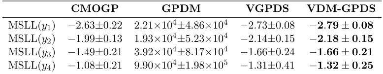
MSLL(y1) −2.63±0.22 2.21×10⁴±4.86×10⁴ −2.73±0.08 −2.79±0.08
MSLL(y2) −1.99±0.13 1.93×10⁴±5.23×10⁴ −2.14±0.15 −2.18±0.15
MSLL(y3) −1.49±0.21 3.92×10⁴±8.17×10⁴ −1.66±0.24 −1.66±0.21
MSLL(y4) −1.08±0.21 9.90×10⁴±1.98×10⁵ −1.31±0.41 −1.32±0.25
Table 2: Averaged MSLL with the standard deviation for predictions on the output-dependent synthetic data.
where κfd,fd0(x,x
0) defined in (12) is the multi-output covariance function. In this paper,
the number of the latent functions in (9) is set to one, i.e.,K = 1, which is also the common setting used in ´Alvarez and Lawrence (2011).
We sample the synthetic data by two steps. First we use the differential equation with parameters γ = 0.5, σ = 0.01 to sample N = 200, Q= 2 latent variables at time interval [−1,1]. Then we sample D = 4 dimensional outputs, each of which has 200 observations through the multi-output GP with the following parameters S1,1 = 1, S2,1 = 2, S3,1 = 3,
S4,1 = 4, P1 = [5,1]>, P2 = [5,1]>, P3 = [3,1]>, P4 = [2,1]> and Λ = [4,5]>. For
approximation, 30 random inducing points are used. In addition, white Gaussian noise is added to each output.
6.1.1 Prediction
Here we evaluate the performance of our method for predicting the outputs given only time over the synthetic data. We randomly select 50 points from each output for training with the remaining 150 points for testing. This is repeated for ten times. The CMOGP, GPDM and VGPDS are performed as comparisons. The cubic spline interpolation (spline for short) is also chosen as a baseline. The latent variables X in the GPDM, VGPDS and VDM-GPDS with two dimensions are initialized by using the principal component analysis on the observations. Moreover, the Mat´ern 3/2 covariance function is used in the VGPDS and VDM-GPDS.
−0.5 0 0.5 1 2
2.5 3 3.5
Time−t
Value−y
Pred True
(a) Spline
−0.5 0 0.5 1
2 2.5 3 3.5
Time−t
Value−y
Pred True
(b) CMOGP
−0.5 0 0.5 1
2 2.5 3 3.5
Time−t
Value−y
Pred True
(c) GPDM
−0.5 0 0.5 1
2 2.5 3 3.5
Time−t
Value−y
Pred True
(d) VGPDS
−0.5 0 0.5 1
2 2.5 3 3.5
Time−t
Value−y
Pred True
(e) VDM-GPDS
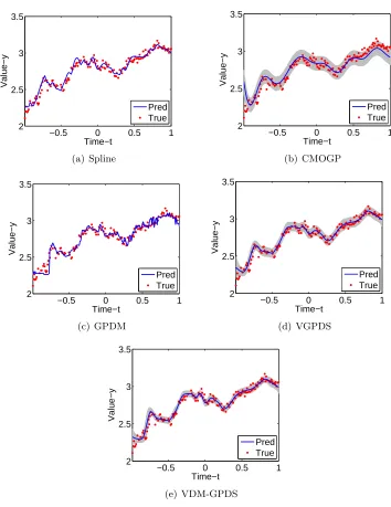
Figure 2: Predictions for y4(t) with the five methods. Pred and True indicate predicted
and observed values, respectively. The shaded regions represent two standard deviations for the predictions.
Spline CMOGP GPDM VGPDS VDM-GPDS
RMSE(y1) 3.81±0.82 11.49±0.26 3.82±1.55 2.18±0.06 2.21±0.06
RMSE(y2) 2.58±0.68 3.59±0.72 3.45±1.70 2.06±0.19 2.05±0.13
RMSE(y3) 3.26±0.90 1.75±0.10 3.57±1.71 1.68±0.09 1.72±0.12
RMSE(y4) 9.06±1.17 8.34±10.89 7.10±1.28 4.48±0.23 4.45±0.20
Table 3: Averaged RMSE (%) with the standard deviation (%) for predictions on the output-independent synthetic data.
CMOGP GPDM VGPDS VDM-GPDS
MSLL(y1) −0.74±0.02 5.22×10²±5.23×10² −2.34±0.04 −2.33±0.04
MSLL(y2) −1.91±0.24 1.10×10³±2.22×10³ −2.36±0.10 −2.36±0.13
MSLL(y3) −2.62±0.05 2.10×10²±3.43×10² −2.50±0.08 −2.52±0.11
MSLL(y4) −1.38±0.66 5.19×10²±1.16×10³ −1.46±0.17 −1.48±0.18
Table 4: Averaged MSLL with the standard deviation for predictions on the output-independent synthetic data.
the GPDM cannot work well in the case in which data on many time intervals are lost. Prediction with the GPDM results in very high MSLL. To sum up, our model gives the best performance among the five models as expected.
In order to give intuitive representations, we draw one prediction result from the ten experiments in Figure 2 where the shaded regions in 2(b), 2(c), 2(d) and 2(e) represent two standard deviations for the predictions. Through the figures, it is clear that the VDM-GPDS has higher accuracies and smaller variances. Note that the GPDM has very small variances, but low accuracies, which leads to the high MSLL as in Table 2. With all the evaluation measures considered, the VDM-GPDS gives the best performance of prediction with only time as inputs.
In addition, to verify the flexibility of the VDM-GPDS, we perform experiments on the output-independent data which are generated analogously to Section 6.1. In particular, the output-independent data are generated using Equation (41) but with κfd,fd0(x,x
0) = 0 for
d6=d0 after generatingX. Note that the GPDM and VGPDS do not make the assumption of output dependency. The results in terms of RMSE and MSLL are shown in Table 3 and Table 4 where we can see that our model performs as well as the VGPDS and significantly better than the CMOGP and GPDM.
6.1.2 Reconstruction
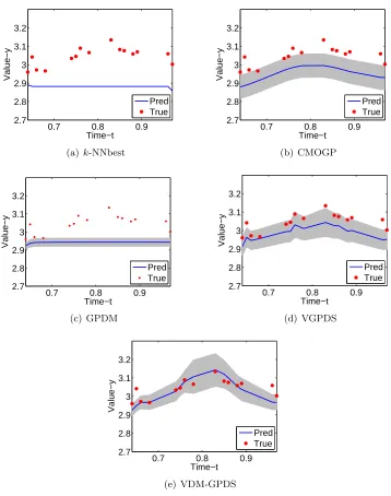
In this section, we compare the VDM-GPDS with the k-nearest neighbor best (k-NNbest) method which chooses the best k from {1, . . . ,5}, the CMOGP, GPDM and VGPDS for recovering missing points given time and partially observed outputs. We set S4,1 =−4 to
generate data in this part, which makes the output y4 be negatively correlated with the
k-NNbest CMOGP GPDM VGPDS VDM-GPDS
RMSE(y1) 1.87±0.62 1.90±0.31 2.69±3.67 1.49±0.94 0.98±0.34
RMSE(y4) 13.51±2.54 9.31±0.87 12.61±2.43 6.79±6.07 5.56±1.88
Table 5: Averaged RMSE (%) with the standard deviation (%) for reconstructions of the missing points fory1 and y4.
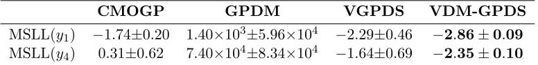
CMOGP GPDM VGPDS VDM-GPDS
MSLL(y1) −1.74±0.20 1.40×10³±5.96×10⁴ −2.29±0.46 −2.86±0.09
MSLL(y4) 0.31±0.62 7.40×10⁴±8.34×10⁴ −1.64±0.69 −2.35±0.10
Table 6: Averaged MSLL with the standard deviation for reconstructions of the missing points fory1 and y4.
resulting in 35 points as training data. Note that the CMOGP considers all the present outputs as the training set while the GPDM, VGPDS and VDM-GPDS only consider the outputs at time interval [−1,0.5) as the training set.
Table 5 and Table 6 show the averaged RMSE and MSLL with the standard deviation for reconstructions of the missing points for y1 and y4. The proposed model performs best
with the lowest RMSE and MSLL. Specifically, our model can make full use of the present data on some dimensions to reconstruct the missing data through the dependency among outputs. This advantage is shown by comparing with the GPDM and VGPDS. In addition, the two Gaussian process mappings in the VDM-GPDS help to well model the dynamical characteristics and complexity of the data. This advantage is shown by comparing to the CMOGP.
Figure 3 shows one reconstruction result fory4 from the ten experiments by five different
methods. It can be seen that the results of the VDM-GPDS are the closest to the true values among the compared methods. This indicates the superior performance of our model for the reconstruction task.
6.2 Human Motion Capture Data
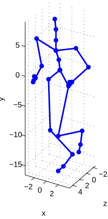
In order to demonstrate the validity of the proposed model on real-world data, we employ ten sequences of runs/jogs from subject 35 (see Figure 4 for a skeleton) and two sequences of runs/jogs from subject 16 in the CMU motion capture database for the reconstruction task. In particular, our task is to reconstruct the right leg or the upper body of one test sequence on the motion capture data given training sequences. We preprocess the data as in Lawrence (2007) and divide the sequences into training and test data. Nine independent training sequences are all from subject 35 and the remaining three testing sequences are from subject 35 and subject 16 (one from subject 35 and two from subject 16). The average length of each sequence is 40 frames and the output dimension is 59.
0.7 0.8 0.9 2.7
2.8 2.9 3 3.1 3.2
Time−t
Value−y
Pred True
(a)k-NNbest
0.7 0.8 0.9
2.7 2.8 2.9 3 3.1 3.2
Time−t
Value−y
Pred True
(b) CMOGP
0.7 0.8 0.9
2.7 2.8 2.9 3 3.1 3.2
Time−t
Value−y
Pred True
(c) GPDM
0.7 0.8 0.9
2.7 2.8 2.9 3 3.1 3.2
Time−t
Value−y
Pred True
(d) VGPDS
0.7 0.8 0.9
2.7 2.8 2.9 3 3.1 3.2
Time−t
Value−y
Pred True
(e) VDM-GPDS
Figure 3: Reconstructions of the missing points for y4(t) with the five methods. Pred and
True indicate predicted and observed values, respectively. The shaded regions represent two standard deviations for the predictions.
block-−2 0 2
−2 0 2 4 −15
−10 −5 0 5
z x
y
Figure 4: A skeleton of subject 35 running at a moment.
NN sc. NN CMOGP GPDM VGPDS VDM-GPDS
RMSE(LS) 0.82 0.85 1.15 0.68 0.65 0.64
RMSE(LA) 6.75 7.94 13.53 5.61 5.54 5.30
RMSE(BS) 1.00 1.40 3.56 0.68 0.66 0.60
RMSE(BA) 5.63 9.57 5.02 3.39 2.81 2.60
RMSE(LS) 1.03 1.40 1.37 0.91 0.89 0.85
RMSE(LA) 10.10 9.73 15.19 8.90 8.13 8.65
RMSE(BS) 2.88 3.00 4.70 2.85 3.80 2.83
RMSE(BA) 7.45 7.83 8.04 7.13 10.64 6.69
Table 7: The RMSE for reconstructions of the missing points of the motion capture data. The values listed above the double line are the results for the one test sequence from subject 35 while the values listed below the double line are the averaged results for the two test sequences from subject 16.
diagonal matrix because the sequences are independent. Moreover, the latent variables X
in the VGPDS and VDM-GPDS with nine dimensions are initialized by using principal component analysis on the observations. For parameter optimization of the VDM-GPDS and VGPDS, the maximum numbers of iteration steps are set to be identical.
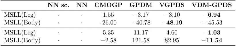
NN sc. NN CMOGP GPDM VGPDS VDM-GPDS
MSLL(Leg) · · 1.55 −3.17 −3.10 −6.94
MSLL(Body) · · -26.00 −40.78 −48.19 −45.53
MSLL(Leg) · · 5.35 11.17 4.60 −1.03
MSLL(Body) · · −2.58 121.58 82.95 −11.54
Table 8: The MSLL for reconstructions of the missing points of the motion capture data. The values listed above the double line are the results for the one test sequence from subject 35 while the values listed below the double line are the averaged results for the two test sequences from subject 16.
BA correspond to the reconstructions of the upper body in the same two spaces. Table 8 shows the MSLL in the original space for the same reconstructions as in Table 7. As expected, the results on subjects whose motions are used to learn the models show signifi-cantly smaller RMSE and MSLL than those for the test motions from subjects not used in the training set. No matter under what circumstances, our model generally outperforms the other approaches. We conjecture that this is because the VDM-GPDS effectively considers both the dynamical characteristics and the dependency among the outputs in the complex dynamical system. Specifically, for the CMU data, the dependency among different parts of the entire body can be well captured by the VDM-GPDS. When only parts of data on each frame of the test sequence are observed, the missing data on the corresponding frame can be recovered by utilizing the observed data. Meanwhile, the GP prior on the latent variables makes sure the continuity and smoothness of movements.
6.3 Traffic Flow Forecasting
The problem addressed here is to predict the future traffic flows of a certain road link. We focus on the short-term predictions, in the time interval of 15 minutes, which is a difficult but very important application. A real urban transportation network is used for this experiment. The raw data are of 25 days, which include 2400 recording points for each road link. Note that the data are not continuous in these 25 days, though data are complete within each recording day. Specifically, the day numbers with recordings are {[1∼19],[21],[25∼29]}. The first seven days are used for training, and the remaining 18 days are for testing. Figure 5 shows a patch taken from the urban traffic map of highways as in Sun et al. (2006). Each circle node in the sketch map denotes a road link. An arrow shows the direction of the traffic flow, which reaches the corresponding road link from its upstream link. Paths without arrows are of no traffic flow records.
We predict the traffic volumes (vehicles/hour) of the road links (Bb,Ch,Dd,Eb, F e,
B
C
D
H
G
F
E
I
J
K
a
b
h
e
f
g
d
b
a
c
i
b
l
k
b
a
c
d
f
h
b
a
d
d
f
c
e
h
b
d
g
Figure 5: A patch taken from the urban traffic map of highways.
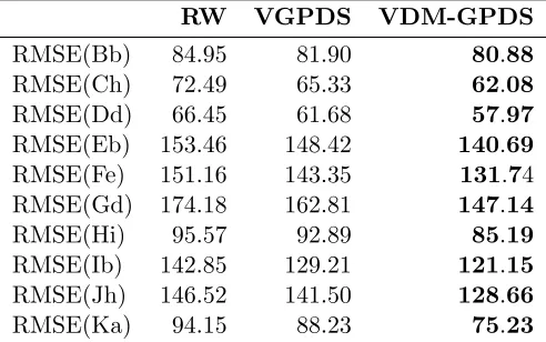
RW VGPDS VDM-GPDS
RMSE(Bb) 84.95 81.90 80.88
RMSE(Ch) 72.49 65.33 62.08
RMSE(Dd) 66.45 61.68 57.97
RMSE(Eb) 153.46 148.42 140.69
RMSE(Fe) 151.16 143.35 131.74
RMSE(Gd) 174.18 162.81 147.14
RMSE(Hi) 95.57 92.89 85.19
RMSE(Ib) 142.85 129.21 121.15
RMSE(Jh) 146.52 141.50 128.66
RMSE(Ka) 94.15 88.23 75.23
Table 9: The RMSE for forecasting results on the traffic flow data.
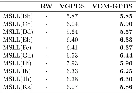
the historic traffic flows of the four road links to predict the flows ofGdin the next interval. The historic time for forecasting is fixed as four intervals. We compare our model with the Random Walk (RW) and VGPDS. The RW is to forecast the current value using the last value (Williams, 1999), which is chosen as a baseline. According to the descriptions about real-time forecasting in Section 4.2, the VGPDS can be adapted to apply to this experiment. Moreover, in the previous experiments, the VGPDS performs best among the compared models except the VDM-GPDS. Therefore, it is sufficient to compare our model with the RW and VGPDS. Note that the realization of the VGPDS also takes the periodicity into consideration.
multi-RW VGPDS VDM-GPDS
MSLL(Bb) · 5.87 5.85
MSLL(Ch) · 6.04 5.90
MSLL(Dd) · 5.64 5.57
MSLL(Eb) · 6.40 6.33
MSLL(Fe) · 6.41 6.37
MSLL(Gd) · 6.53 6.44
MSLL(Hi) · 5.93 5.90
MSLL(Ib) · 6.33 6.25
MSLL(Jh) · 6.38 6.30
MSLL(Ka) · 6.07 5.86
Table 10: The MSLL for forecasting results on the traffic flow data.
output dependency in the VDM-GPDS; the relationship between the traffic flows of the objective road link and its own historical series is captured by the dynamical characteristics modeled in the VDM-GPDS. Therefore, the entire cause information is well collected by the VDM-GPDS to predict the traffic flows of the objective road link.
To be intuitive, we give the final forecasting results of the performed models for the road link Gd in the last three days in Figure 6. The VDM-GPDS has shown great superiority to the compared models. As seen from Figure 6(a) and Figure 6(b), the forecasting results with the RW and VGPDS often lag.
6.4 Robot Inverse Dynamics Problem
The robot inverse dynamics problem is an important task in the robot areas (Sciavicco and Vijayakumar, 2000). For a goal of touching or grasping a subject using a robotic manipu-lator, it usually needs the following procedures. First, the inverse kinematic calculates the robot joint coordinates given the pose of the end-effector. Then trajectory planing decides a trajectory describing how a robot should move to achieve the desired task. Finally, given the trajectory, i.e., the motion specified by the joint angles, velocities and accelerations, the torques needed at the joints to drive it along the trajectory are computed by the inverse dynamics. What we concerned here is the robot inverse dynamics problem. Analytical models for the inverse dynamics are often infeasible, for example due to uncertainty in the physical parameters of the robot, or the difficulty of modeling frictions. This leads to the need to learn the inverse dynamics by some machine learning methods (Chai et al., 2009; Nguyen and Bonilla, 2014).
0 50 100 150 200 250 300 0
500 1000 1500 2000 2500
Sample point
Traffic flow (veh/h)
True Pred
(a) RW
0 50 100 150 200 250 300 0
500 1000 1500 2000 2500
Sample point
Traffic flow (veh/h)
True Pred
(b) VGPDS
0 50 100 150 200 250 300 0
500 1000 1500 2000 2500
Sample point
Traffic flow (veh/h)
True Pred
(c) VDM-GPDS
Figure 6: Forecasting results of the performed models for the road linkGdon the last three days.
learning for the two couples, the 2nd and 3rd, the 4th and 7th torques. Note that, the 2nd and 3rd torques are negatively correlated while the 4th and 7th torques are positively correlated.
Joint 2 Joint 1
Joint 3 Joint 4
Joint 5
Joint 6
Joint 7
Figure 7: Sketch of the SARCOS dextrous arm (Vijayakumar and Schaal, 2000).
Method 2nd joint 3rd joint
(N = 100) RMSE MSLL RMSE MSLL
sGPR 6.33±1.33 3.85±0.86 4.48±1.04 4.06±1.18
MTGP 5.52±0.79 3.88±0.19 3.20±0.38 3.10±0.27
COGP 5.11±0.44 4.17±0.69 3.18±0.23 3.39±0.38
VGPDS 4.89±0.36 6.20±0.87 2.96±0.26 5.73±0.89
VDM-GPDS 4.55±0.34 2.95±0.14 2.68±0.22 2.34±0.15
Method 4th joint 7th joint
(N = 100) RMSE MSLL RMSE MSLL
sGPR 5.01±2.06 4.33±1.54 1.04±0.22 2.76±1.53
MTGP 3.27±0.35 3.44±0.49 0.72±0.07 2.11±0.55
COGP 3.26±0.25 2.68±0.24 0.68±0.05 1.30±0.21
VGPDS 3.19±0.20 2.36±0.08 0.65±0.03 0.86±0.66
VDM-GPDS 3.19±0.26 2.44±0.12 0.66±0.04 0.95±0.10
Table 11: Averaged RMSE and MSLL with the standard deviation for robot inverse dy-namics learning with 100 training points.
30 inducing points are used for 100, 300 and 500 training points, respectively. For the VDM-GPDS and VGPDS, the dimensionality of the latent space is set to two. Table 11, 12 and 13 show the results for different methods in terms of averaged RMSE and MSLL. For intuition, we also plot the RMSE results in Figure 8.
VDM-Method 2nd joint 3rd joint
(N = 300) RMSE MSLL RMSE MSLL
sGPR 4.19±0.83 2.85±0.32 2.61±0.51 2.44±0.37
MTGP 4.37±0.89 3.36±0.35 2.53±0.56 2.77±0.19
COGP 3.78±0.14 5.08±0.79 2.27±0.09 3.49±0.43
VGPDS 3.67±0.18 2.62±0.04 2.11±0.12 2.06±0.04
VDM-GPDS 3.52±0.09 2.59±0.04 2.01±0.06 2.00±0.03
Method 4th joint 7th joint
(N = 300) RMSE MSLL RMSE MSLL
sGPR 2.21±0.37 2.39±0.59 0.55±0.13 0.92±0.51
MTGP 2.01±0.20 2.40±0.12 0.47±0.04 1.27±0.19
COGP 2.25±0.18 2.65±0.25 0.52±0.02 1.71±0.21
VGPDS 2.31±0.38 2.12±0.15 0.48±0.06 0.59±0.10
VDM-GPDS 1.95±0.09 1.92±0.04 0.45±0.01 0.53±0.04
Table 12: Averaged RMSE and MSLL with the standard deviation for robot inverse dy-namics learning with 300 training points.
Method 2nd joint 3rd joint
(N = 500) RMSE MSLL RMSE MSLL
sGPR 4.01±0.71 2.78±0.27 2.08±0.45 2.05±0.32
MTGP 3.50±0.32 3.42±0.27 1.97±0.27 2.59±0.24
COGP 3.33±0.08 5.24±0.49 1.89±0.06 3.54±0.34
VGPDS 3.47±0.17 2.57±0.03 1.98±0.12 2.02±0.03
VDM-GPDS 3.20±0.11 2.52±0.04 1.77±0.08 1.93±0.04
Method 4th joint 7th joint
(N = 500) RMSE MSLL RMSE MSLL
sGPR 2.08±0.38 2.28±0.51 0.47±0.08 0.76±0.45
MTGP 1.66±0.17 2.28±0.19 0.39±0.02 1.27±0.15
COGP 1.77±0.06 2.46±0.10 0.45±0.02 2.20±0.22
VGPDS 1.93±0.14 2.04±0.08 0.44±0.01 0.55±0.04
VDM-GPDS 1.64±0.06 1.83±0.02 0.39±0.01 0.44±0.03
Table 13: Averaged RMSE and MSLL with the standard deviation for robot inverse dy-namics learning with 500 training points.
100 300 500 0
1 2 3 4 5 6 7 8
RMSE
Training Set Size
sGPR MTGP COGP VGPDS VDM−GPDS
(a) 2nd joint
100 300 500 0
1 2 3 4 5 6
RMSE
Training Set Size
sGPR MTGP COGP VGPDS VDM−GPDS
(b) 3rd joint
100 300 500 0
1 2 3 4 5 6 7 8
RMSE
Training Set Size
sGPR MTGP COGP VGPDS VDM−GPDS
(c) 4th joint
100 300 500
0 0.2 0.4 0.6 0.8 1 1.2 1.4
RMSE
Training Set Size
sGPR MTGP COGP VGPDS VDM−GPDS
(d) 7th joint
Figure 8: Averaged RMSE with the standard deviation for the 2nd, 3rd, 4th and 7th joint torques prediction. (better in color)
the multiple outputs. No matter for dynamical system modeling or static data regression, the proposed model is reasonable and applicable.
6.5 Performance and Efficiency Analysis
The proposed VDM-GPDS outperforms several previous methods for predicting outputs and recovering missing points for dynamical systems. In order to quantify the superior results, we evaluate the performance increases with the averaged performance increasing ratio to the VGPDS in terms of RMSE. The increasing ratios of the four experiments (Sections 6.1.1, 6.1.2, 6.2, 6.3 and 6.4) are 4.49%, 26.17%, 10.40%, 7.35% and 7.97%, respectively.
CMOGP GPDM VGPDS VDM-GPDS
computational complexity O(D3N3) O(N3) O(M2N Q) O(M2N DQK)
execution time 50.7 26.8 74.2 181.1
Table 14: Computational complexities and execution time (in ms) for different models.
since the proposed method explicitly models the dependency among outputs, the dependent multi-output covariance matrix in the VDM-GPDS is a full matrix with sizeN D×N D and operations involving it cannot be factorized. This is in contrast to the independent multi-output covariance matrix in the GPDM and VGPDS, which is block-diagonal. As in Titsias (2009), inducing points are employed for the variational inference for the VDM-GPDS. The number of the inducing points M is much smaller than that of the data points N, which can improve the computational efficiency. For the VDM-GPDS, the most time-consuming calculation is to compute ψ2 whose computational complexity isO(M2N DQK).
In order to give clear comparisons in terms of efficiency, we list the computational complexities of four models and the execution time (in ms) of one step for learning the models on the synthetic data in Table 14. Through the table, we find that the VDM-GPDS costs a lot. Nevertheless, our model can obtain high performance improvements as discussed above. We believe that getting performance improvements is worth the time cost.
7. Conclusion
In this paper, we have proposed a dependent multi-output GP for modeling complex dynam-ical systems. We give the reasonable assumption that the different outputs of the systems are generally dependent. The convolved process covariance function is employed to model the dependency among all the data points across all the outputs. We adapt the variational inference method involving inducing points to our model so that the latent variables are variationally integrated out. The model and variational parameters are jointly optimized with the scaled conjugate gradient method. Through small adaptations, our model can handle regression problems.
Modeling the possible dependency among multiple outputs can help to make better predictions. The effectiveness of the proposed model for complex dynamical systems is empirically demonstrated through multiple experiments. However, when the dimensionality of the output is very high, our model may take a long time to converge. This opens the possibility for future work to accelerate training for high dimensional dynamical systems.
Acknowledgments
Appendix A. Derivation of the Lower Bound
In order to approximately compute the marginal likelihood p(Y|t), we compute the varia-tional lower bound of it by involving the variavaria-tional distribution q(F, U, X|Z). The varia-tional lower bound Lcan be expressed as
L=
Z
q(F, U, X|Z) logp(Y, F, U, X|t, Z)
q(F, U, X|Z) dXdU dF
=
Z
p(f|u, X, Z)q(u)q(X) logp(y|f)p(u|Z)p(X|t)
q(u)q(X) dfdudX,
(42)
since
p(Y, F, U, X|t, Z) =p(y|f)p(f|u, X, Z)p(u|Z)p(X|t), (43) and
q(F, U, X|Z) =p(f|u, X, Z)q(u)q(X). (44) For neatness, the above expression is split into two parts as L = ˆL −KL[q(X)||p(X|t)]. Specifically, ˆLis expressed by
ˆ L=
Z
p(f|u, X, Z)q(u)q(X) logp(y|f)p(u|Z)
q(u) dfdudX. (45)
KL[q(X)||p(X|t)] is the relative entropy of q(X) and p(X|t), expressed as
KL[q(X)||p(X|t)] =
Z
q(X) log q(X)
p(X|t) =Q
2 log|Kt,t| − 1 2
Q
X
q=1
log|Sq|
+1 2
Q
X
q=1
[Tr(K−1t,tSq) + Tr(Kt−1,tµqµ>q)] +const,
(46)
since
p(X|t) = Q
Y
q=1
N(xq|0,Kt,t), (47)
and
q(X) = Q
Y
q=1
N(xq|µq, Sq). (48)
So far,KL[q(X)||p(X|t)] can be calculated analytically as the above, we need to calculate ˆ
L. By using the facts that logp(y|f)q(u)p(u|Z) = logp(y|f) + logp(u|q(u)Z) andR p(f|u, X, Z)df = 1, ˆ
L is converted into
ˆ L=
Z
q(u)q(X)
Z
p(f|u, X, Z) logp(y|f)dfdudX
+
Z
q(u)q(X) logp(u|Z)
q(u) dudX.
We know thatp(y|f) and p(f|u, X, Z) are both Gaussian, and then
Z
p(f|u, X, Z) logp(y|f)df
= logN(y|Kf,uK−1u,uu, β−1I)−
β
2Tr(Kf,f −Kf,uK
−1 u,uKu,f).
(50)
Thus ˆL in (49) can be simplified as
ˆ L=
Z
q(u)q(X) logN(y|a, B)p(u)
q(u) dudX
−
Z
β
2Tr(Kf,f −Kf,uK
−1
u,uKu,f)q(X)dX,
(51)
wherea=Kf,uK−1u,uu andB =β−1I. By changing the integration order, we get
ˆ L=
Z
q(u)[loge
hlogN(y|a,B)iq(X)
p(u)
q(u) ]d(u) −β
2Tr(hKf,fiq(X)− hKf,uK
−1
u,uKu,fiq(X)).
(52)
We compute the optimal bound using the reserved Jensen’s inequality as in Titsias and Lawrence (2010). This gives
ˆ L ≤log
Z
ehlogN(y|a,B)iq(X)p(u)du − β
2Tr(hKf,fiq(X)) +
β
2Tr(hKf,uK
−1
u,uKu,fiq(X)).
(53)
The optimal distribution q(u) that gives rise to this lower bound is given by q(u) =
ehlogN(y|Kf,uK−u,1uu,β−1I)iq(X)p(u), which is analytically Gaussian
q(u)∝ N(βy>ψ1Ku,u(βψ2+Ku,u)−1ψ1>y,Ku,u(βψ2+Ku,u)−1), (54)
where ψ0 = Tr(hKf,fiq(X)), ψ1 =hKf,uiq(X) and ψ2 =hKu,fKf,uiq(X). The closed-form of
the lower bound of the approximated marginal log-likelihood defined as Lis given by
L= log
"
βN D2 |Ku,u| 1 2
|2π|N D2 |βψ2+Ku,u| 1 2
exp{−1 2y
>
Wy}
#
−βψ0
2 +
β
2Tr(K
−1
u,uψ2)−KL[q(X)||p(X|t)],
(55)
whereW =βI−β2ψ1(βψ2+Ku,u)−1ψ1>. Given the above, we can obtain the final
Appendix B. Gradients with Respect to the Parameters
The parameters involved in the proposed model include the model parameters {β,θx,θf} and the variational parameters{{µ¯q, λq}Qq=1, Z}after reparameterizing{µq, Sq}Qq=1. All the
parameters are jointly optimized by maximizing the lower bound in (21) with the scaled conjugate gradient method. Here we give the detailed gradients of all the parameters. Note that in our model the dimensionality of the latent variableU is one (K=1). So the statistics such as Sd,k, Λk, W are changed to sd, Λ, M here. In order to simplify the expressions, we define Σψ0 = 2Pd+ Λ, Σψ1 = Pd+ Λ +Sn, Σψ21 = 2(Pd+ Λ), Σψ22 =
Pd+Λ
2 +Sn,
C−1=β−1Ku,u+ψ2. z is equivalent tozmand z0 is equivalent tozm0. The symbol|q after
a matrix means theqth column of the matrix.
Because of the reparameterization, we need to calculate the gradients of ˆLwith respect to µq, Sq and then obtain the gradients of L with respect to ¯µq, λq using (28) and (29). Given that KL[q(X)||p(X|t)] does not involve the parameters θf, β and Z, its gradients with respect toθf,β and Z are zero. Therefore, ∂∂θLf = ∂
ˆ L
∂θf,
∂L
∂β = ∂Lˆ
∂β and ∂L
∂Z = ∂Lˆ
∂Z.
First, we give the gradients of ˆLwith respect to µq,Sq,Pd,sd through the formulation
∂Lˆ
∂θ =−
β
2
∂ψ0
∂θ +βTr[ ∂ψ>1
∂θ yy
>ψ 1C] +
β
2Tr[
∂ψ2
∂θ (K
−1 u,u−
C
β −Cψ
>
1 yy>ψ1C)], (56)
where θ represents µnq, Snq, Pdq and sd. The detailed derivatives of ψ0, ψ1 and ψ2 with
respect to µnq, Snq, Pdq and sd are different. The derivatives of ψ0, (ψ1)vm and (ψ2)mm0
with respect toµnq are
∂ψ0
∂µnq = 0,
∂(ψ1)vm
∂µnq
=sdN(z|µn,Σψ1)((z−µn) >
Σ−1ψ
1|q),
∂(ψ2)mm0 ∂µnq
= D
X
d=1
sd2N(z|z0,Σψ21)N( z+z0
2 |µn,Σψ22)(( z+z0
2 −µn)
>
Σ−1ψ
22|q).
(57)
The derivatives of ψ0, (ψ1)vm and (ψ2)mm0 with respect toSnq are ∂ψ0
∂Snq = 0,
∂(ψ1)vm
∂Snq
=sdN(z|µn,Σψ1)(− |Σψ1|
−1
2
∂|Σψ1|
∂Snq −1
2(z−µn)
>∂Σ −1
ψ1
∂Snq
(z−µn)), ∂(ψ2)mm0
∂Snq =
D
X
d=1
sd2N(z|z0,Σψ21)N( z+z0
2 |µn,Σψ22)
(−|Σψ22| −1
2
∂|Σψ22|
∂Snq − 1
2(
z+z0
2 −µn)
>∂Σ −1
ψ22
∂Snq
(z+z
0
2 −µn)).
The derivatives of ψ0, (ψ1)vm and (ψ2)mm0 with respect toPdq are ∂ψ0 ∂Pdq = D X d=1 −N 2
sdsd
|2π|Q2|Σψ 0|
3 2
∂|Σψ0|
∂Pdq
,
∂(ψ1)vm
∂Pdq
=sdN(z|µn,Σψ1)(− |Σψ1|
−1
2
∂|Σψ1|
∂Pdq −1
2(z−µn)
>∂Σ −1
ψ1
∂Pdq
(z−µn)),
∂(ψ2)mm0 ∂Pdq
= N
X
n=1
sd2N(z|z0,Σψ21)N( z+z0
2 |µn,Σψ22)
(−|Σψ21| −1
2
∂|Σψ21|
∂Pdq − 1
2(z−z
0)>∂Σ −1
ψ21
∂Pdq
(z−z0)
−|Σψ22| −1
2
∂|Σψ22|
∂Pdq −1
2(
z+z0
2 −µn)
>∂Σ −1
ψ22
∂Pdq
(z+z
0
2 −µn)).
(59)
The derivatives of ψ0, (ψ1)vm and (ψ2)mm0 with respect tosd are
∂ψ0
∂sd
= 2N sd |2π|Q2|Σψ
0| 1 2
,
∂(ψ1)vm
∂sd
=N(z|µn,Σψ1),
∂(ψ2)mm0 ∂sd
= N
X
n=1
2sdN(z|z0,Σψ21)N( z+z0
2 |µn,Σψ22).
(60)
Then, we give the gradients of L with respect to Λ and Z through the formulation
∂L
∂θ =−
β
2
∂ψ0
∂θ +βTr[ ∂ψ1>
∂θ yy
Tψ
1C] +
β
2Tr[
∂ψ2
∂θ (K
−1 u,u−Cψ
> 1 yy
>
ψ1C−β−1C)]
+ 1 2Tr[
∂Ku,u
∂θ (K
−1 u,u−Cψ
> 1yy
>
ψ1C−β−1C−βK−1u,uψ2K −1 u,u],
(61)
whereθrepresents Λq,Zmq. The detailed derivatives of theψ0,ψ1,ψ2andKu,uwith respect
to Λq, Zmq are given separately. The derivatives of ψ0, (ψ1)vm, (ψ2)mm0 and (Ku,u)
with respect to Λq are
∂ψ0
∂Λq = D
X
d=1
−N 2
sdsd
|2π|Q2|Σψ 0|
3 2
∂|Σψ0|
∂Λq ,
∂(ψ1)vm
∂Λq
=sdN(z|µn,Σψ1)(−
1 2|Σψ1|
−1∂|Σψ1|
∂Λq −1
2(z−µn)
>∂Σ −1
ψ1
∂Λq
(z−µn)), ∂(ψ2)mm0
∂Λq = N X n=1 D X d=1
sd2N(z|z0,Σψ21)N( z+z0
2 |µn,Σψ22)
(− ∂|Σψ21|
2|Σψ21|∂Λq −1
2(z−z
0)>∂Σ −1
ψ21
∂Λq (z−z
0)
− ∂|Σψ22|
2|Σψ22|∂Λq −1
2(
z+z0
2 −µn)
>∂Σ −1
ψ22
∂Λq
(z+z
0
2 −µn)),
∂(Ku,u)mm0 ∂Λq
=N(z|z0,Λ)(−1 2|Λ|
−1∂|Λ|
∂Λq −1
2(z−z
0)>∂Λ−1
∂Λq
(z−z0)).
(62)
The derivatives of ψ0, (ψ1)vm, (ψ2)mm0 and (Ku,u)
mm0 with respect to zmq are
∂ψ0
∂zmq =0,
∂(ψ1)vm
∂zmq
=−sdN(z|µn,Σψ1)((z−µn) >
Σ−1ψ
1|q),
∂(ψ2)mm0 ∂zmq
= D
X
d=1
sd2N(z|z0,Σψ21)N( z+z0
2 |µn,Σψ22)
(−1 2(
z+z0
2 −µn)
>Σ−1
ψ22|q+ (z−z 0)>Σ−1
ψ21|q),
∂(Ku,u)mm0 ∂zmq
=− 1 ΛqN(z|z
0,Λ)(z
mq−zm0q).
(63)
Finally, we give the gradients ofL with respect toβ and θx as follows.
∂L
∂β =
1 2[Tr(K
−1
u,uψ2) + (V −M)β−1−ψ0−Tr(yy>) + Tr(Cψ1>yy>ψ1)
+β−2Tr(Ku,uC) +β−1Tr(Ku,uCψ>1yy>ψ1C)], (64)
∂L ∂θx = Q X q=1
Tr[[−1
2( ˆBqKt,t ˆ
Bq+ ¯µqµ¯Tq) + (I−BˆqKt,t)
∂Lˆ
∂Sq
(I−BˆqKt,t)>]
∂Kt,t
∂θx ]
+ ∂Lˆ
∂µq
!>
∂Kt,t
∂θx ¯
µq, (65)
where ˆBq= Λ
1 2
q(I+ Λ
1 2
qKt,tΛ 1 2
q)−1Λ
1 2
Appendix C. Derivations of Prediction with Only Time
With the parameters as well as time t and t∗ omitted, the posterior density for prediction is given by
p(Y∗|Y) = Z
p(Y∗|F∗)p(F∗|X∗, Y)p(X∗|Y)dF∗dX∗, (66)
where F∗ ∈ RN∗×D denotes the set of latent variables (the noise-free version of Y∗) and
X∗∈RN∗×Q represents the latent variables in the low dimensional space.
The distribution p(F∗|X∗, Y) in (66) is approximated by the variational distribution
p(F∗|X∗, Y)≈q(f∗|X∗) = Z
p(f∗|u, X∗)q(u)du, (67)
wheref∗>= [f∗1>, ...,f∗>D], andp(f∗|u, X∗) is Gaussian with the formulation
p(f∗|u, X∗) =N(f∗|Kf∗,uK
−1
u,uu,Kf∗,f∗−Kf∗,uK
−1
u,uKu,f∗). (68)
Since the optimal setting forq(u) in our variational framework is also found to be Gaussian,
q(f∗|X∗) is Gaussian that can be computed analytically
q(f∗|X∗) =N(βKf∗,u(Ku,u+βψ2)
−1
ψ>1y,
Kf∗,u(Ku,u+βψ2)
−1K>
f∗,u+Kf∗,f∗−Kf∗,u,K
−1
u,uK>f∗,u).
(69)
The distributionp(X∗|Y) in (66) is approximated by the variational distributionq(X∗)
which is Gaussian and can be explicitly formulated as
q(X∗) =N(µX∗,ΣX∗), (70)
whereµX∗ is composed of column vectorµx∗q and block-diagonal matrixΣX∗ has diagonal
elementΣx∗q with
µx∗q = Kt∗,tK
−1
t,tµq, (71)
Σx∗q = Kt∗,t∗−Kt∗,tK
−1
t,t(Kt,t∗−SqK
−1
t,tKt,t∗). (72)
Given p(F∗|X∗, Y) approximated by q(f∗|X∗) and p(X∗|Y) approximated byq(X∗), the
posterior density of f∗ (the noise-free version ofy∗) is now approximated by
p(f∗|Y) =
Z
q(f∗|X∗)q(X∗)dX∗. (73)
So far, following Damianou et al. (2011), the expectation of f∗and its element-wise autoco-variance are given in (33) and (34).
References