Convex Regression with Interpretable Sharp Partitions
Ashley Petersen [email protected]
Noah Simon [email protected]
Department of Biostatistics University of Washington Seattle, WA 98195
Daniela Witten [email protected]
Departments of Biostatistics and Statistics University of Washington
Seattle, WA 98195
Editor:Maya Gupta
Abstract
We consider the problem of predicting an outcome variable on the basis of a small number of covariates, using an interpretable yet non-additive model. We proposeconvex regression with interpretable sharp partitions (CRISP) for this task. CRISP partitions the covariate space into blocks in a data-adaptive way, and fits a mean model within each block. Unlike other partitioning methods, CRISP is fit using a non-greedy approach by solving a convex optimization problem, resulting in low-variance fits. We explore the properties of CRISP, and evaluate its performance in a simulation study and on a housing price data set.
Keywords: convex optimization, interpretability, non-additivity, non-parametric regres-sion, prediction
1. Introduction
Classification and regression trees (CART) are immensely popular for flexible and non-additive predictive modeling, despite the fact that they date back more than thirty years (Breiman et al., 1984). The trees are fit using a two-stage process in which the tree is first greedily “grown” to some maximum size, and then “pruned” to avoid overfitting. The final tree with K terminal nodes can be visually displayed as a decision tree with K −1 splits, or equivalently as K disjoint boxes that completely partition the covariate space. CART has stood the test of time, because its output is highly interpretable and it can easily incorporate complex non-additive relationships between features. However, it is a greedy procedure, and a small perturbation of the data can produce a very different tree. The high variability of the fitted values can compromise the scientific utility of the tree, as well as the tree’s prediction accuracy on test data. While an ensemble approach, like random forests, can reduce CART’s variability, this comes at the expense of interpretability (Breiman, 2001).
greedily chosen and some of which involve pairs of features. TPS fits the observed data, regularized by smoothness penalties. In the case of two covariatesx1 andx2and a response y, the TPS fit is the solution to
minimize
f
n
X
i=1
[yi−f(x1i, x2i)]2+λ
Z Z
R2
k∇2f(x
1, x2)k2F dx1 dx2.
The fits from MARS and TPS are incredibly flexible, but can be less interpretable than the fits from CART.
In recent years, the statistical community has been very interested in formulating pre-dictive models as solutions to convex optimization problems. However, to the best of our knowledge, no proposals have been made for flexible, non-additive, and interpretable mod-eling via convex optimization. To close this gap, we propose a non-greedy procedure whose fits have a block structure reminiscent of CART. Our proposal, convex regression with in-terpretable sharp partitions (CRISP), is the solution to a convex optimization problem with predictions that are much less variable than those of CART. Also unlike CART, CRISP bor-rows information across the blocks, and is able to adequately model the data when the mean model is smooth. Thus our method provides a compromise between the interpretability of CART and the flexibility of MARS and TPS. In this paper, we consider the low-dimensional setting in which there are a small number of covariates of interest (p n). We leave an extension to the p > nsetting to future work.
CRISP has a number of attractive properties:
• CRISP can accommodate interactions between pairs of covariates in a flexible way. This is useful when the impact of one covariate may depend on the value of another covariate, but there is not stronga prioriknowledge about the form of the interaction.
• CRISP fits a piecewise constant model, which is easily interpreted by even those with limited statistical background.
• CRISP is formulated as a convex optimization problem. Thus we can solve for the global optimum, and can derive an expression for CRISP’s degrees of freedom.
The remainder of this paper is organized as follows. In Section 2, we introduce our method and present an algorithm to implement it. We compare our method to existing approaches using simulated data in Section 3. In Section 4, we derive some properties of the method. In Section 5, we discuss connections between our method and other work. We illustrate our method on a housing price data set in Section 6. We consider a modification to our proposal in Section 7, and close with the discussion in Section 8. Proofs are in the Appendix.
2. Convex Regression with Interpretable Sharp Partitions
Throughout most of this paper, for ease of exposition, we focus on the case ofp= 2 features. An extension to the case of p >2 is given in Section 7.
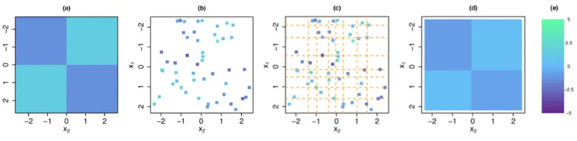
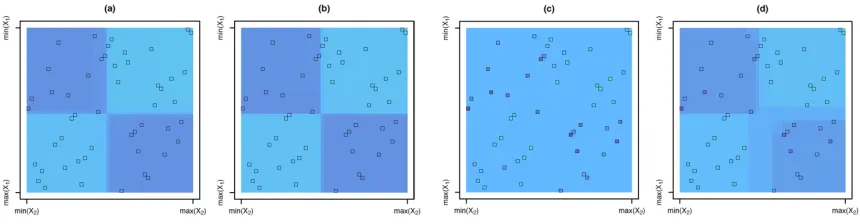
Figure 1: In (a), the mean model f(x1, x2) used to generate data. In (b), each of the 50 squares represents an observation (x1, x2, y) with y = f(x1, x2) + with ∼ N(0,1). In (c), there are q2 = 64 bins of (x1, x2) values, whose boundaries coincide with the octiles ( ) of x1 and x2. In (d), CRISP estimatesf(x1, x2) to be constant within each bin, and furthermore encourages adjacent bins to take on the same value. When applied to the data in(b) with q = 8, this leads to an estimatedf(x1, x2) with four blocks. In(e), we show the heat scale legend.
error term, andf is an unknown function that we wish to estimate. An example off(x1, x2) is displayed in Figure 1(a). Figure 1(b) displays a training set of n i.i.d. observations of (x1, x2, y). We first partition the feature space into q2 bins, as shown in Figure 1(c) with q= 8. The CRISP approach estimatesf(x1, x2) to be constant within each bin, and further encouragesf to take on the same value at adjacent bins; this leads to constant-valuedblocks. The CRISP output is shown in Figure 1(d); there are four estimated blocks. More details about this simulation set-up are provided in Section 3.
2.1 Notation and Goal of CRISP
We now introduce some new notation, and provide further intuition for CRISP, before presenting the optimization problem for CRISP in Section 2.2.
As is shown in Figure 1(c), we wish to estimate the mean modelf(x1, x2) for aq×q grid of bins, wheref(x1, x2) is estimated to be constant within each bin. LetM ∈Rq×q denote
a mean matrix whose elementM(i)(j)contains the mean for pairs of covariate values within aquantile rangeof the observed predictorsx1,x2∈Rn. For example,M(1)(2)represents the mean of the observations withx1 less than the 1q-quantile ofx1, andx2 between the 1q- and
2
q-quantiles ofx2. In Figure 1(c), the corner grid bins correspond toM(1)(1),M(8)(1),M(8)(8), and M(1)(8), starting at the top-left corner of the grid and moving counter-clockwise. In CRISP, our goal is to estimate theq×q matrixM on the basis of y∈Rn, which contains
nnoisy observations from various bins of M.
to an estimated mean model with a block structure. For instance, in Figure 1(d), M is estimated to have four blocks, or regions of feature space over which f(x1, x2) is constant. Consequently, the CRISP solution M∗ shown in Figure 1(d) only has 4 unique elements, while M is an 8×8 matrix. If we examined the estimateM∗, we would see that all pairs of neighboring rows and neighboring columns of M∗ are identical, except for one pair of columns and one pair of rows.
While the true mean model in this example has a block structure (as seen in Figure 1(a)), we will show in Section 3 that CRISP can perform well even when the true mean model is smooth. The data in this example were uniformly distributed in the covariate space. CRISP is most suitable for data applications where observations are distributed throughout the covariate space. Highly correlated covariates will lead to an insufficient amount of data to estimate the mean model over the entire covariate space.
2.2 The Optimization Problem
The CRISP optimization problem balances the trade-off between fitting the data and en-couraging a block structure. We estimate M by solving the convex optimization problem
minimize
M∈Rq×q
1 2
n
X
i=1
(yi−Ω(M, x1i, x2i))2+λP(M). (1)
In (1), the function Ω extracts the element of M corresponding to the bin to which the observation (x1i, x2i) belongs. For instance, in Figure 1(c), Ω(M,0,−1) = M(4)(2). Note that Ω is explicitly defined in Appendix A. Furthermore, λ≥0 is a tuning parameter, and the penalty P is defined as
P(M) =
q−1
X
i=1
h
Mi·−M(i+1)·
2+
M·i−M·(i+1)
2
i
, (2)
whereMi·andM·i denote theith row and column ofM, respectively. The sum of squared
errors in (1) encourages the estimate of M to fit the data, while the group lasso penalty (Yuan and Lin, 2006) in (2) encourages pairs of neighboring rows (or columns) to be exactly identical. This leads to the formation of constant-valued blocks, which are comprised of multiple bins of theq×qgrid. Appendix B discusses other possible penalties that could be used in (1).
We now rewrite (1) in a way that will be useful later. We introduce a vectorized form of M, which is denoted by m = vec(M) = (M·1)T, (M·2)T, · · ·, (M·q)T
T
where M·i
is the ith column of M. The correspondence between M and m is shown in Figure 10 of Appendix A. In what follows, we will switch between using the matrix M and the vectorizedm. Then (1) can be rewritten as
minimize
m∈Rq2
1
2ky−Qmk 2 2+λ
q−1
X
i=1
[kRimk2+kCimk2], (3)
where each row of Q ∈ Rn×q2 contains q2−1 elements that equal 0, and a single 1, such
of x1 and x2, we suppress this to simplify the notation.) In (3), Ri,Ci ∈ Rq×q
2
extract differences between neighboring rows and columns of M (i.e., Rim =Mi·−M(i+1)· and Cim = M·i −M·(i+1)). An example of Q and explicit definitions of Q, Ri, and Ci are
in Appendix A. We let A = RT
1, · · · , RTq−1, C1T, · · · , CqT−1
T
∈ R2q(q−1)×q2
, and then rewrite (3) as
minimize
m∈Rq2,z∈R2q(q−1)
1
2ky−Qmk 2 2+λ
q−1
X
i=1
[kz1ik2+kz2ik2] subject to Am=z, (4)
wherez = (z11)T, · · · , (z1(q−1))T, (z21)T, · · ·, (z2(q−1))T
T
withz1i,z2i ∈Rq.
While (1), (3), and (4) have the same solution, it is most convenient to derive an algorithm to solve CRISP using the parameterization in (4). Throughout this paper, we will alternate between using the notation M∗ andm∗, wherem∗ = vec(M∗), to represent the CRISP solution to (4). The training set predictions for CRISP are given by ˆy=Qm∗.
2.3 An Algorithm for CRISP
We solve for the global optimum of the convex optimization problem (4) using thealternating directions method of multipliers(ADMM) algorithm (Boyd et al., 2011). This is summarized in Algorithm 1. Additional details are in Appendix C.
Algorithm 1 — Alternating Directions Method of Multipliers for Equation (4)
1. Let u = (u11)T, . . . , (u1(q−1))T, (u21)T, . . . , (u2(q−1))T
T
denote the scaled dual variables. Initializem(0):=0,z(0):=0,and u(0) :=0.
2. Fork= 1,2, . . ., until the primal and dual residuals satisfy a stopping criterion:
(a) m(k):=QTQ+ρATA−1QTy+ρAT(z(k−1)−u(k−1)) (b) z1(ki):= (Rim(k)+u(k
−1)
1i )(1−λ/(ρkRim(k)+u(k
−1) 1i k2))+,
z2(ki):= (Cim(k)+u(k
−1)
2i )(1−λ/(ρkCim(k)+u(k
−1)
2i k2))+ fori= 1, . . . , q−1 (c) u(k):=u(k−1)+Am(k)−z(k)
In Algorithm 1, the computational bottleneck occurs in Step 2(a). Evaluating the q -banded matrixQTQ+ρATAhas a one-time cost ofO(n+q4) operations, and computing its LU factorization requires an additionalO(q4) operations. Then Step 2(a) can be performed in O(q3) operations (Boyd and Vandenberghe, 2004). Therefore, Algorithm 1 requires an initial step of O(n+q4) operations, followed by a per-iteration complexity of O(q3).
On a Macbook Pro with a 2.0 GHz Intel Sandy Bridge Core i7 processor, our Python
We chose to solve CRISP using an ADMM algorithm, as ADMM works well in related problems. For example, in the context of trend filtering, Ramdas and Tibshirani (forth-coming) found that their ADMM implementation converged more reliably across a variety of tuning parameter values and sample sizes than the primal-dual interior point method of Kim et al. (2009). In our setting, an interior point algorithm for CRISP involves solving a dense system of equations at each iteration, which has a computational complexity of O(q6). Additionally, an interior point method would not recover the exact block structure (any strictly feasible solution would have no zero row or column differences). In contrast, we directly recover the block structure of our estimated mean model from the z variables of our ADMM algorithm. Furthermore, ADMM algorithms typically converge to moder-ate accuracy within only tens of iterations (Boyd et al., 2011), which is acceptable in our setting.
The value of λ can be chosen using K-fold cross-validation. Alternatively, λ can be selected using approaches based on Akaike’s information criterion (AIC; Akaike, 1973) or Bayesian information criterion (BIC; Schwarz, 1978) using the degrees of freedom estimator proposed in Section 4.1. The roles of λ and q in controlling the granularity of the model are further characterized in Sections 4.2 and 4.3.
3. Simulations
In this section, we compare the performance of CRISP to CART, TPS, and competing methods. We consider a variety of mean models, as well as smaller (n= 100) and larger (n= 10,000) training set sample sizes.
3.1 Methods
We generate data with either n = 100 or n = 10,000, and p = 2. We independently sample each element of x1 and x2 from a Unif[−2.5,2.5] distribution, and then take y = f(x1,x2) +, where∼MVN(0, σ2In) withσ = 1 forn= 100 and σ= 10 for n= 10,000.
Note that we use the notation MVN to indicate a multivariate normal distribution.
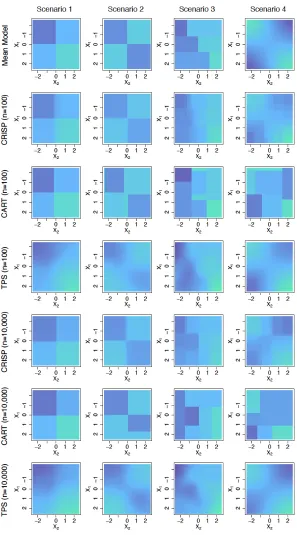
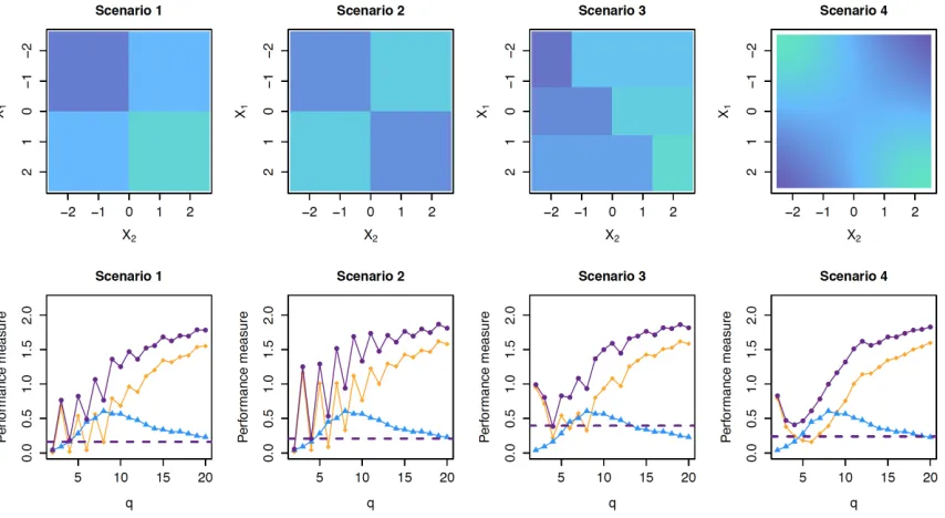
We consider four mean models for f(x1, x2); these are displayed in the top panel of Figure 2, and defined in detail in Appendix D. In Scenario 1, the mean model is additive inx1 andx2. Scenario 2 is similar to Scenario 1, but the mean model is non-additive. The mean model in Scenario 3 is piecewise constant, with the cut points for x2 depending on
x1. Finally, Scenario 4 is a smooth mean model.
For each of the four scenarios, we plot mean squared prediction error1 versus degrees of freedom (a notion that will be discussed extensively in Section 4.1). CRISP and FLAM are fit over a sequence of exponentially decreasing λ values, with the degrees of freedom estimated using (6) and a result from Petersen et al. (forthcoming), respectively. TPS is fit over a sequence of degrees of freedom. For CART, we vary the number of terminal nodes in the tree, and average the estimator (7) over the replicates in order to estimate the degrees of freedom for each number of terminal nodes. Note that the number of degrees of freedom of CART is non-monotonic for small numbers of terminal nodes (as seen in Figure 3).
3.2 Results for n= 100
Results are shown in Figure 3. We see that both CRISP and TPS perform reasonably well in terms of prediction error in all scenarios, regardless of the true mean model. FLAM outperforms the other methods in Scenario 1, which is unsurprising as the mean model is truly additive, and FLAM boils down to CRISP with an additivity constraint (Section 5.2). However, FLAM performs poorly for mean models with substantial non-additivity (Scenar-ios 2 and 4). Outside of Scenario 1, CART performs worse than TPS and CRISP. CRISP, TPS, and CART all perform better than a linear model with an interaction in Scenarios 1–3. However, in Scenario 4, the mean model is well-approximated using a linear model. We also fit MARS for all scenarios; however, performance was poor and the results are omitted.
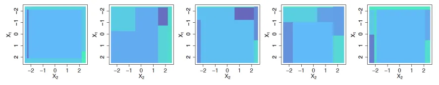
While CRISP and TPS have comparable prediction error, their fits are quite different. In Figure 2, we show the estimated mean models for CRISP, TPS, and CART for a single replicate of data in each scenario. CRISP provides fits that reflect the true mean model well, even when the true mean model is smooth. While TPS has low prediction error, the smooth fits from TPS are not easily interpreted and are far from the true mean model in some scenarios. While the fits from CART reflect the mean model reasonably well in Scenarios 1 and 2, the fits from CART in all scenarios are highly variable. CART fits from different replicates of Scenario 4 are shown in Figure 4. The average variance of an element ofM∗ across the 200 replicates for Scenario 4 was 0.843 for CART, compared to 0.0935 for CRISP and 0.0653 for TPS. The variance of CART’s fitted values is similarly inflated for the other scenarios. Small perturbations of the data can produce very different qualitative conclusions when examining CART’s fits.
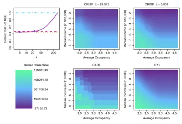
3.3 Results for n= 10,000
We compare CRISP to TPS and CART. Results are in Figures 2 and 5. Again, CRISP performs well in all scenarios, and the CART fits are much more variable than those of CRISP and TPS. The average variance of an element of M∗ across the 200 replicates for Scenario 1 was 0.111 for CART, compared to 0.051 for CRISP and 0.083 for TPS. For Scenario 2, the average variance was 1.42 for CART, compared to 0.056 for CRISP and 0.083 for TPS. For Scenario 3, the average variance was 0.692 for CART, compared to 0.077 for CRISP and 0.129 for TPS. And finally, for Scenario 4, the average variance was 1.89 for
1. Mean squared prediction error is defined as 1
q2kM−M
∗k2
F, whereM∈R q×q
is the true mean matrix and
Mean Squared Prediction Error
0 5 10 15 20 25 30 35
0.0
1.0
2.0
3.0
Scenario 1
Degrees of Freedom
*
*
*
0 5 10 15 20 25 30 35
0.0
1.0
2.0
3.0
Scenario 2
Degrees of Freedom
*
*
*
0 5 10 15 20 25 30 35
0.0
1.0
2.0
3.0
Scenario 3
Degrees of Freedom
*
*
*
0 5 10 15 20 25 30 35
0.0
1.0
2.0
3.0
Scenario 4
Degrees of Freedom
*
*
*
Figure 3: Mean squared prediction error, as a function of the degrees of freedom, for the four scenarios considered in the simulations of Section 3.2. The methods displayed are CRISP ( ), FLAM ( ), TPS ( ), CART ( ), linear model with an interaction ( ), and the oracle linear model ( ). The oracle linear model is only fit for Scenarios 1–3, for which the mean models have constant regions. Shaded bands (only visible for CART) indicate point-wise 95% confidence intervals over the 200 replicate data sets. The linear models have a fixed number of degrees of freedom, but are shown as horizontal lines. Asterisks indicate the degrees of freedom used for the fits shown in Figure 2.
Mean Squared Prediction Error
0 10 20 30 40
0.0
1.0
2.0
3.0
Scenario 1
Degrees of Freedom
*
*
*
0 10 20 30 40
0.0
1.0
2.0
3.0
Scenario 2
Degrees of Freedom
*
*
*
0 10 20 30 40
0.0
1.0
2.0
3.0
Scenario 3
Degrees of Freedom
*
*
*
0 10 20 30 40
0.0
1.0
2.0
3.0
Scenario 4
Degrees of Freedom
*
*
*
Figure 5: Results for n= 10,000 for CRISP ( ), TPS ( ), and CART ( ) in the simu-lations of Section 3.3. Details are as given in Figure 3.
CART, compared to 0.096 for CRISP and 0.061 for TPS. Notably, a large sample size is not sufficient for producing stable CART fits, unless the signal-to-noise ratio is suitably large.
4. Properties of CRISP
In this section, we provide an unbiased estimator for CRISP’s degrees of freedom. We also derive an analytical expression for the range ofλfor which the solution to (4) takes a constant value, m∗ = n11Ty
1. Lastly, we discuss the role of q and λ in controlling the granularity of CRISP. Throughout this section, we use A+ to denote the Moore-Penrose pseudoinverse of a matrix A.
4.1 Degrees of Freedom
Suppose that Var(y) =σ2I, and letg(y) = ˆydenote the fit corresponding to some model-fitting procedure g. Then the degrees of freedom of g is defined as σ12
Pn
i=1Cov(yi,yˆi)
(Hastie and Tibshirani, 1990; Efron, 1986).
The concept of degrees of freedom provides a common framework for comparing the complexities of various models; this is particularly useful when the models under consider-ation are complex or unrelated. Ye (1998) proposed a computconsider-ationally-burdensome Monte Carlo approach for estimating the degrees of freedom of a model-fitting procedure. In recent years, unbiased estimators for the degrees of freedom have been derived for the lasso and generalized lasso (Zou et al., 2007; Tibshirani and Taylor, 2012), among other methods. These estimators allow us to characterize a model’s complexity, and also can be used in order to develop an approach for tuning parameter selection based on Akaike’s information criterion (AIC; Akaike, 1973) or Bayesian information criterion (BIC; Schwarz, 1978).
Problem (3) is equivalent to the problem
minimize
m
1
2ky−Qmk 2
2+λ
q−1 X
i=1
[kRimk2+kCimk2] + γ 2kmk
2
2 (5)
We now introduce some notation. First, we define C, the set of difference matrices corresponding to equal neighboring rows or columns in the solution m∗ to (5). That is, C ={Ai :kAim∗k2 = 0} where A1 = R1,A2 =R2, . . . ,Aq−1 =Rq−1,Aq = C1,Aq+1 =
C2, . . . ,A2q−2 =Cq−1.Then we defineA∗ to be the submatrix ofA obtained by retaining
only the rows ofAcorresponding to matricesAi ∈ C. Note thatA∗∈Rq|C|×q2. We propose
to estimate the degrees of freedom of CRISP as
ˆ
dfCRISP = Tr
Q
D+λP X
i:Ai∈C/
S2(Ai,m∗)P +γI
−1
P QT
, (6)
whereP =Iq2 −A+∗A∗,S2(Ai,m∗) = A
T iAi
kAim∗k2 −
AT
iAim∗m∗TATiAi
kAim∗k32
, and Qwas defined in
(3). Recall that M∗ will tend to contain row-column blocks of constant value, as shown in Figure 1(d). We defineD = diag
h(m∗1),· · ·, h(m∗q2)
, where h(m∗i) is the ratio of the number of observations in the block of M∗ that contains m∗i to the number of elements of M∗ in the block of M∗ that contains m∗i. We use the notation MVN to indicate a multivariate normal distribution.
Proposition 1 Assume y∼MVN(µ, σ2I). Then dfˆCRISP is an unbiased estimator of the degrees of freedom of CRISP.
The following corollary indicates that the estimator (6) simplifies substantially when the CRISP solution takes a particular form.
Corollary 2 Assume y∼MVN(µ, σ2I). If either all rows or all columns ofM∗ are equal, then the total number of blocks of M∗ is an unbiased estimator of the degrees of freedom.
In 100 replicate data sets withyi ∼N(µi, σ2), we compare the mean of (6) to the mean
of
1 σ2
n
X
i=1
(ˆyi−µi) (yi−µi), (7)
which provides a Monte Carlo estimate of σ12 Pn
i=1Cov(yi,yˆi), the true degrees of freedom
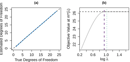
of CRISP. The results in Figure 6(a) empirically validate Proposition 1, showing that (6) is an unbiased estimator of CRISP’s degrees of freedom. Note that the proofs of Proposition 1 and Corollary 2 can be found in Appendices E and F, respectively.
4.2 Range of λ that Yields a Constant Solution
CRISP has a single tuning parameter λ, which we typically will select via cross-validation or a related approach. Here, we derive the minimum value ofλsuch that m∗= 1n1Ty1, corresponding to a fit in which all elements of m∗ are equal.
Lemma 3 The solution to (4) is constant (i.e., m∗ = n11Ty1) if and only if λ≥ max
1≤i≤q−1{kd
∗
0 5 10 15 20 25
0
5
10
15
20
25
(a)
True Degrees of Freedom
Estimated Degrees of Freedom 0.2 0.6 1.0 1.4
22
23
24
25
26
(b)
log λ
Objectiv
e V
alue at m*(
λ
)
Figure 6: In (a), we compare the degrees of freedom calculated using our estimator (7) (y-axis) from Section 4.1 to the unbiased, Monte Carlo estimator (6) (x-axis). Varying λ gives the solid line, and the dashed line indicates y = x. In (b), we plot the value of the objective of (4) at m∗(λ), the minimizer of (4) at λ, for a replicate of data as λvaries. We compare two ways of finding a λ large enough such that m∗(λ) = 1n1Ty
1, which results in the objective shown as . We take λ = max1≤i≤q−1{kd1ik2,kd2ik2} with either d being the solution to (8) ( ) or d = (AT)+QT y− 1
n1 Ty
1 ( ). The former ( ) matches the result of Lemma 3 in Section 4.2.
where d∗ = (d∗11T · · · d∗1(Tq−1)d∗21T . . . d∗2(Tq−1))T is the solution to minimize
d 1≤maxi≤q−1{kd1ik2,kd2ik2} subject to Q
T
y−
1 n1
Ty
1
=ATd. (8)
Recall that the matrix Q was defined in (3). Takingλ= max1≤i≤q−1
n
kd˜1ik2,kd˜2ik2
o
for
any feasible vector ˜dfor (8) will give a value of λsufficiently large so m∗ is constant. For example, we can choose ˜d= (AT)+QT y− n11Ty1. However, choosingλin accordance with Lemma 3 will give the minimum value of λ such that m∗ = 1n1Ty
1. The opti-mization problem (8) can be solved using a standard convex solver, such as SDPT3 via
CVX in MATLAB (Grant and Boyd, 2008, 2014). An illustration of Lemma 3 is provided in
Figure 6(b).
4.3 Controlling the Granularity of CRISP
Both q and λcontrol the granularity of the final CRISP model: q controls the size of the grid used to construct M, and λ controls the number of blocks in the final fitted CRISP model. For a range of very small λ values, there will beq2 blocks; for larger λ values, the CRISP solution will have a smaller number of blocks.
4.3.1 Choice of q
In principle,q may be chosen to equaln. This means that each bin of theq×q grid would contain at most one observation. However, when n is large, choosing q = n can lead to excessive computational time, memory burden, and variance in the fit. Instead, we aim to choose q to be large enough to allow for adequate granularity, but not excessively large. What constitutes adequate granularity will depend on the context of the problem.
In our analyses, we choose to treat q as a fixed parameter that is chosen prior to fitting CRISP. However, if desired,q could be chosen byK-fold cross validation.
4.3.2 Choice of λ
To illustrate the role ofλ, consider takingλ= 0 in (3), and treatingqas a tuning parameter rather than a fixed value. When λ= 0, (3) contains only a sum of squared errors term, so the estimate within each bin is the mean value of the observations in that bin. For bins without any observations, we estimate the corresponding element of M to be the overall mean ofy.
For the mean models shown in Figure 2, we compare CRISP to (3) with λ = 0 and q chosen adaptively. We focus on the general findings here, but detailed results are given in Appendix H. When the true mean model is piecewise constant with boundaries that are well-approximated by a grid of bins (as in Scenarios 1–3), CRISP and (3) with λ = 0 and variable q perform similarly. However, CRISP is clearly superior at estimating the smooth mean model of Scenario 4 (Figure 12), as it is able to borrow information across bins, instead of simply fitting the mean of observations within each bin. CRISP also allows the granularity of the fitted model to vary adaptively over the covariate space, as shown in Figure 13(a) of Appendix H. The blocks of this mean model perfectly align with a grid that hasq = 3, but the mean model only has 4 blocks. While (3) withλ= 0 andq= 3 fits 9 blocks, CRISP correctly identifies 4 blocks (Figures 13(b) and 13(c) of Appendix H).
5. Connections to Other Methods
In this section, we establish connections between CRISP and two previous proposals.
5.1 Connection to One-Dimensional Fused Lasso
Suppose that for a given value of λ, the CRISP fit involves only one covariate: that is,
M∗ = ˜m1Tq or M∗ = 1qm˜T for some ˜m ∈ Rq. We will now show that in this setting,
the CRISP solution can be recovered by solving a one-dimensional fused lasso problem (Tibshirani et al., 2005).
Before presenting Lemma 4, we introduce some notation. DefineD= [I(q−1)×(q−1) 0(q−1)×1]− [0(q−1)×1 I(q−1)×(q−1)] to be the first difference matrix. Define ˜y ∈ Rq such that ˜yi is the
mean outcome value of the observations in theith row of theq×q grid used to construct
M. Let ni denote the number of observations in the ith row of the q×q grid used to
constructM. DefineW ∈Rq×q to be the diagonal matrix with entries√n
1, √
Lemma 4 Suppose that, for some value ofλ, the CRISP solution is of the formM∗ = ˜m1Tq for some m˜ ∈Rq. Then m˜ is the solution to the problem
minimize ˜
m∈Rq
1
2kW( ˜y−m˜)k 2 2+λ
√
qkDm˜k1. (9)
If insteadM∗ =1qm˜T, then a result similar to Lemma 4 holds, with modifications to the
definitions of W and ˜y.
Equation 9 is a weighted fused lasso problem with response vector ˜y and weights √
n1, √
n2, . . . ,√nq. When q =n, (9) simplifies to a standard one-dimensional fused lasso
problem.
Corollary 5 If q = n and M∗ = ˜m1Tn, then m˜ is the solution to the one-dimensional fused lasso problem
minimize ˜
m∈Rn
1
2kP y−m˜k 2 2+λ
√
nkDm˜k1, (10) where P is the permutation matrix that orders the elements of x1 from least to greatest. If instead M∗ = 1nm˜T, then Corollary 5 holds with P defined to be the permutation
matrix that orders the elements of x2 from least to greatest. 5.2 Connection to Fused Lasso Additive Model
In this subsection, we will establish that CRISP is a generalization of the fused lasso additive model (FLAM) proposal of Petersen et al. (forthcoming). FLAM fits an additive model in which each covariate’s fit is estimated to be piecewise constant with adaptively-chosen knots. For simplicity, assume thatq=n. Consider a modification of CRISP in which we impose additivity on the mean matrix M. That is, we assume f(x1, x2) = θ0 +f1(x1) +f2(x2), whereθ0is an overall mean, andf1 andf2 are mean-zero over the training observations. We introduce then-vectorsθ1 andθ2, wheref1(xi1) =θ1i and f2(xi2) =θ2i for alli= 1, . . . , n.
Thus the additivity constraint for the (i, j) element of M,M(i)(j), can be expressed as M(i)(j) =θ0+θ1i+θ2j fori= 1, . . . , n; j = 1, . . . , n with 1Tθ1 =1Tθ2= 0. (11) Lemma 6 CRISP (1)–(2) with q=n and with the additional additivity constraint (11) is equivalent to FLAM with p= 2, which is the solution to the optimization problem
minimize
θ0∈R,θ1,θ2∈Rn 1
2ky−(θ01+θ1+θ2)k 2
2+λ(kDP1θ1k1+kDP2θ2k1) subject to 1Tθ1=1Tθ2 =0,
(12)
where λ≥0 is a tuning parameter, Pj is the permutation matrix that orders the elements
of xj from least to greatest, and D = [I(n−1)×(n−1) 0(n−1)×1]−[0(n−1)×1 I(n−1)×(n−1)] is the first difference matrix.
The proof of Lemma 6 follows from algebraic manipulation.
CRISP (1)–(2) with the additivity constraint (11) is also equivalent to FLAM when the `2 norms in the penalty (2) are changed to`1 or`∞norms. These alternative penalties are
discussed further in Appendix B.
6. Data Application
We consider predicting median house value on the basis of median income and average occupancy, measured for 20,640 neighborhoods in California. The data set was originally considered in Pace and Barry (1997) and is publicly available from the Carnegie Mellon StatLib data repository (lib.stat.cmu.edu).
For this analysis, we focus on predicting median house value for the central area of the covariate space. In particular, we filter the neighborhoods to select those with median incomes and average occupancies that both fall within the central 95% of the covariate distribution, which results in 18,662 neighborhoods to be analyzed. Further details are provided in Appendix I. To illustrate the impact that the size of the data set may have on the preferred analysis approach, we consider five different training set sizes: 100, 500, 1000, 5000, and 11,198 (which corresponds to 60% of the observations). We use the observations not selected for the training set as the test set. For each training set size, we consider 10 different data samples. We compare the performance of CRISP (with q = 100) to CART and TPS.
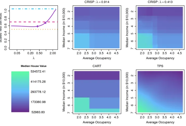
Figure 7 shows that income is positively associated with house value. Occupancy is not strongly associated with house value in low-income neighborhoods. However, among neighborhoods with median incomes exceeding around $50,000, neighborhoods with mostly single or double occupancy tend to have more expensive homes than those with higher occupancies and the same income. This is perhaps because single people and couples without children have more disposable income to spend on housing than families at the same income level.
In Figure 7, we show estimated mean models from CRISP for two different values of λ. The larger value ofλhas slightly worse prediction performance, but has a simple block structure reminiscent of CART. The smaller value ofλgives better prediction performance with a more complex fit structure that resembles the fits from TPS. This illustrates how CRISP’s tuning parameter,λ, balances the trade-off between interpretability and prediction performance.
0 2000 6000 10000
0.0e+00
1.5e+09
3.0e+09
Size of training set
A
v
er
age V
ar
iance of Element of M* ●
●● ●
●
●
●●
● ●
●
●● ● ●
0 2000 6000 10000
0.0
0.2
0.4
0.6
Size of training set
Minim
um Scaled T
est Set MSE
●
●● ● ●
●
● ●
● ●
●
●● ● ●
Figure 8: We plot the average variance of predictions and the minimum scaled test set MSE (as defined in Figure 7) as a function of training set sample size for CRISP ( ), CART ( ), and TPS ( ) applied to the housing data considered in Section 6.
7. Extension to p >2
We have assumed thus far thatp= 2. In this case, the estimated mean model for the entire covariate space can be summarized in a single plot, as in Figure 2.
We extend CRISP to the setting ofp >2 by constructing anadditive model of bivariate fits. That is, we estimate the fit for each of the p(p2−1) pairs of features, giving a bivariate fit for each pair of covariates like those obtained in the setting ofp= 2 and shown in Figure 2. We assume that the mean model is additive in these fits. We restrict the model to pairwise interactions between covariates for a couple of reasons. First, only considering pairwise interactions increases interpretability and reduces model complexity. Our model fit with pairwise interactions can be summarized using p(p2−1) plots, like those shown in Figure 2. There is no analogous way to easily summarize the model if we were to include higher-order interactions. Second, considering higher-order interactions would cause our model to suffer from the curse of dimensionality. That is, as the number of covariates increases, the data in any region of thep-dimensional space will become sparser and sparser: there would be an insufficient density of data throughout the covariate space to reasonably estimate a mean model with higher-order interactions.
We now present the details of our proposal for CRISP with p >2. We consider interac-tions between each pair of features, {(j, j0) : 1≤j < j0 ≤p}. For ease of notation, we refer to the elements of this set using the indexk∈(1, . . . , K) whereK= p(p2−1). Recall that for p= 2, the mean model for CRISP is E[y|x1,x2] =Qm, wherem∈Rq
2
is the vectorized mean matrix and Q selects the elements of m corresponding to the covariate bins of the elements ofy. Recall thatQis a function ofx1 andx2, though we suppress this to simplify the notation. Forp >2, we consider the mean model
E[y|x1, . . . ,xp] =m01+
K
X
k=1
Qkmk,
where m0 ∈ R is an intercept, mk ∈ Rq
2
is the vectorized mean matrix for the pair of features indexed by k, and Qk ∈ Rn×q2 selects the elements of mk corresponding to the
covariate bins for the pair of covariates indexed byk. We include the intercept m0 ∈Rin
our model, and assume thatm1, . . . ,mK are mean-zero, to ensure identifiability.
When p >2, we extend the CRISP optimization problem (4) as follows:
minimize
m0,mk,zk:k=1,...,K
1 2
y− m01+
K
X
k=1
Qkmk
!
2
2 +λ
K
X
k=1
q−1
X
i=1
kzk,1ik2+kzk,2ik2
subject to Amk=zk,1Tmk= 0,
(13)
whereAis as defined in Section 2.2. Thus ˆy=m∗01+PK
k=1Qkm∗k, where (m0∗,m∗1, . . . ,m∗K)
is the solution to (13).
Problem (13) can be solved using block coordinate descent (Tseng, 2001), which gives Algorithm 2. We iterate through the pairs of covariates, and perform a partial minimization (using Algorithm 1) for eachmk, while keeping the others fixed. Using an argument similar
an initial step and O(q3) for each iteration of Step 2(b) of Algorithm 2. In practice, the number of iterations needed to achieve convergence in Step 2(b) of Algorithm 2 is relatively small.
We present a block coordinate descent algorithm, since it is a natural extension of Algorithm 1 to the p > 2 setting. However, CRISP with p 2 can alternatively be fit using generalized gradient descent, which allows the updates for each bivariate fit to be run in parallel on a cluster.
Algorithm 2 — Block Coordinate Descent for CRISP withp >2 (Equation (13))
1. Initialize m∗0 = 0 andm∗k=0 for allk= 1, . . . , K.
2. Fork= 1, . . . , K,1, . . . , K, . . ., until convergence of the objective of (13):
(a) Compute the residualrk=y−
m∗01+P
k06=kQk0m∗ k0
.
(b) Using Algorithm 1, solve
minimize
mk,zk
1
2krk−Qkmkk 2
2+λ
q−1 X
i=1
kzk,1ik2+kzk,2ik2
subject to Amk=zk.
Letm∗k denote the solution.
(c) Compute the intercept, m∗0 ← m∗0 + mean(m∗k), and center, m∗k ← m∗k − mean(m∗k).
8. Discussion
We have presented CRISP, a method for fitting interpretable, flexible, and non-additive predictive models. CRISP fits have an easily-interpreted block structure, which is somewhat reminiscent of the fits from CART. But the fits from CRISP result from a non-greedy procedure, and are much less variable than those of CART. In our numerical studies, the prediction performance of CRISP is similar to TPS, and in many cases CRISP provides a simpler and more interpretable fit.
Future work could consider an alternative penalization scheme. Recall that CRISP first divides the covariate space into aq×qgrid of bins. Our proposal only uses the information about the bin into which each of then observations falls, which is used to construct Q in (4). Thus CRISP only makes use of the rankings of the observations for each covariate, rather than the actual values of the covariates. A modification to (4) could allow us to more heavily penalize the differences between pairs of neighboring rows or columns corresponding to observations with similar values in a given covariate. This modification is not very important when the covariate pairs are distributed uniformly over the covariate space, as in our simulation study in Section 3.
−2 −1 0 1 2
2
1
0
−
1
−
2
(a)
x2
x1
−2 −1 0 1 2
2
1
0
−
1
−
2
(b)
x2
x1
−2 −1 0 1 2
2
1
0
−
1
−
2
(c)
x2
x1
Figure 10: In (a), each of the 20 squares represents an observation (x1, x2, y). There are q2 = 16 bins of (x1, x2) values, whose boundaries coincide with the quartiles ( ) of x1 and x2. In (b) and (c), we label the elements of M and m, respectively, corresponding to each bin of (x1, x2) values. Additionally, in (b) and(c), we show (x1i, x2i) = (0.4,0.8), which is used in Appendix A to describe
the construction ofQ.
Acknowledgments
We thank the associate editor and three referees for helpful comments. D.W. was supported by NIH Grant DP5OD009145, NSF CAREER Award DMS-1252624, and an Alfred P. Sloan Foundation Research Fellowship. N.S. was supported by NIH Grant DP5OD019820.
Appendix A. Notational Details
We first give an intuitive explanation of our vectorization scheme. Recall that each row of
Q ∈Rn×q2
contains q2−1 elements that equal 0, and a single 1 that extracts an element of maccording to the covariate values for that observation. For example, consider the ith row of Q for (x1i, x2i) = (0.4,0.8) in Figure 10(a). These covariate values fall within the
2nd row and 3rd column of the 4×4 grid, meaning thatM(2)(3) provides an estimate foryi.
After vectorizing M,M(2)(3) is m10, the 10th element of the mean vector. Note that we can convert between the matrix and vector notation by taking the column number minus one multiplied byq and adding the row number (e.g., (3−1)×4 + 2). The correspondence betweenM and m is illustrated in Figures 10(b) and 10(c). Thus theith row ofQ would contains all zeros, except a single 1 for the 10th element. Finally, (Qm)i=m10.
Before formally defining the function Ω and matrices Q, Ri for i = 1, . . . , q−1, and Ci for i = 1, . . . , q−1 introduced in Section 2.2, we define a quantile function. We use
quantile(·) to denote the quantile range into which an element falls: quantile(x1i) =kifx1i
We define the function Ω as Ω(M, x1i, x2i) = M(a)(b) where a = quantile(x1i) and
b= quantile(x2i).
We construct Q∈Rn×q2
such that
[Q]jk =
(
1 ifk= quantile(x1j) +q×(quantile(x2j)−1)
0 otherwise ,
Ri ∈Rq×q
2
fori= 1, . . . , q−1 such that
[Ri]jk =
1 ifk=i+q×(j−1) −1 ifk=i+ 1 +q×(j−1)
0 otherwise
,
and Ci ∈Rq×q2 fori= 1, . . . , q−1 such that
[Ci]jk =
1 ifk=j+q×(i−1) −1 ifk=j+q×i
0 otherwise
.
Appendix B. Alternative Penalties
A more general formulation of our proposal in (1) is
minimize
M∈Rq×q
1 2
n X
i=1
(yi−Ω(M, x1i, x2i)) 2
+λ q−1 X
i=1
Mi·−M(i+1)·
t+
M·i−M·(i+1) t
, (14)
which is equivalent to (1) fort= 2. One might consider solving (14) for t=∞, which (like t= 2) encourages pairs of neighboring rows or columns of M to be identical. We compare the fit for t = 2 to that for t =∞ in Figure 11(a)–(b). While t = ∞ gives desirable fits similar to t= 2, the computational time required is much higher than that fort= 2. This is because when adapted to t=∞, Step 2(b) of Algorithm 1 no longer has a closed-form solution (Duchi and Singer, 2009).
We also consider the use of t= 1 in (14); this encourages each element of M to equal its four adjacent elements. However, using t = 1 gives very poor results: the bins of M
containing observations are estimated to be shrunken versions of their observed values, while the bins of M without observations are estimated to be a common value (Figure 11(c)). In a sense, the penalization fort= 1 is too local given the data sparsity (e.g., only q of q2 elements observed whenq=n).
The results fort= 1 improve if an additional penalty is added to the objective function. First, note that (14) can also be written as
minimize
M∈Rq×q
1 2
n
X
i=1
(yi−Ω(M, x1i, x2i))2+λ kMTDTkt,1+kM DTkt,1
, (15)
where D = [I(q−1)×(q−1) 0(q−1)×1]−[0(q−1)×1 I(q−1)×(q−1)]. Motivated by a proposal from van de Geer (2000), we add an additional penalty to (15) witht= 1,
minimize
M∈Rq×q
1 2
n X
i=1
Figure 11: The estimated mean model from solving (14) for(a)t= 2 (CRISP),(b)t=∞, and (c) t= 1, as well as(d) the estimated mean model from solving (16). The methods are described in detail in Appendix B. Note that q = n was used for all methods. Data was generated for n= 50 from Scenario 2 (described in Section 3). The locations of the 50 observations are outlined in each plot. The heat scale legend is in Figure 1(e).
The penalty kDM DTk
1,1 encourages |M(i)(j)+M(i−1)(j−1)−M(i−1)j −Mi(j−1)|to equal zero, which results in a block structure as shown in Figure 11(d). While (16) outperforms (14) with t= 1, CRISP witht= 2 yields better results.
Appendix C. Details of Algorithm 1
C.1 Derivation of Algorithm 1
The scaled augmented Lagrangian of (4) is
Lρ(m,z,u) =
1
2ky−Qmk 2 2+λ
q−1
X
i=1
[kz1ik2+kz2ik2]
+ρ 2
q−1
X
i=1
h
kRim−z1i+u1ik22+kCim−z2i+u2ik22
i
(17)
whereu= (u11)T. . .(u1(q−1))T(u21)T. . .(u2(q−1))T
T
is the scaled dual variable. Solving (4) using ADMM relies on initializing estimates m(0) := 0,z(0) := 0, and u(0) := 0 and then iterating over three steps until convergence. At iterationk, the updates are
Step 1. m(k):= argmin
m
Lρ
m(k−1),z(k−1),u(k−1)
Step 2. z(k):= argmin
z
Lρ
m(k),z(k−1),u(k−1)
Note that Step 3 can equivalently be written asu(k):=u(k−1)+Am(k)−z(k). We provide details regarding Steps 1 and 2 below.
Details of Step 1
The optimality condition of (17) form is
∂Lρ
∂m =−Q
T(y−Qm) +ρ
q−1
X
i=1
RTi (Rim−z1i+u1i) +CiT(Cim−z2i+u2i)
=0
or equivalently,−QT(y−Qm) +ρAT(Am+u−z) =0.Therefore the update for Step 1 ism(k):=
QTQ+ρATA−1
QTy+ρAT(z(k−1)−u(k−1))
.
Details of Step 2
Theproximal operator proxλfofλfis defined byproxλf(v) = argmin
x
f(x) +21λkx−vk2 2
.
The minimization for Step 2 is separable in the z1i and z2i for i= 1, . . . , q−1. The
mini-mization forz1i is
z1(ki):= argmin
z1i
λkz1ik2+ ρ 2
Rim
(k)−z
1i+u(k
−1) 1i 2 2
=proxλ ρk·k2
Rim(k)+u(k
−1) 1i
=
Rim(k)+u(1ki−1)
1−
λ
ρ
Rim
(k)+u(k−1) 1i 2 + .
Similarly, the update forz2i isz2(ki):=
Cim(k)+u(k
−1) 2i
1− λ
ρ
Cim
(k)+u(k−1) 2i 2 ! + .
C.2 Stopping Criterion
We use the stopping criterion for Algorithm 1 suggested in Boyd et al. (2011), stopping when the primal residualr(k) =Am(k)−z(k) and dual residuals(k) =ρAT z(k−1)−z(k)
are sufficiently small. Specifically, we check if
kr(k)k2 ≤
p
2q(q−1)abs+relmax{kAm(k)k2,kz(k)k2} and ks(k)k2 ≤qabs+relkρATu(k)k2 with abs, rel > 0. We use abs = 10−4 and rel = 10−2 in order to obtain the results presented in Sections 3 and 6.
C.3 Varying Penalty Parameter
be updated in conjunction with the updating of ρ. At the end of each iteration, we apply the updates
(ρ(k+1),u(k+1)) :=
(τincrρ(k),u(k)/τincr) ifkr(k)k2 > δks(k)k2 (ρ(k)/τdecr, τdecru(k)) ifks(k)k2 > δkr(k)k2 (ρ(k),u(k)) otherwise
where δ, τincr, τdecr >1. We choose δ = 10 and τincr = τdecr = 2. Updating ρ keeps the
norms of the residualsr(k) and s(k) within a factor of δ of one another. While convergence of ADMM has only been proven for fixed ρ, varying ρ has been shown to work well in practice (Boyd et al., 2011).
C.4 Modification to Provide Sparsity
Inspection of the updates forz∗1iandz∗2iin Algorithm 1 indicates that the ADMM algorithm yields sparsity in z∗1i and z2∗i, but not necessarily exact equality of the rows and columns of M∗. This is in effect a numerical issue: our algorithm might yield z1i =0, but kMi∗·− M(∗i+1)·k2 = 1×10⁻⁸. To resolve this issue, we first determine the “blocks” of m∗ using an initial run of Algorithm 1, and then solve (4) once more with constraints on the rows and columns of M to enforce equality of the appropriate rows and columns. This second optimization is performed simply to yield an estimate ofM for which elements are exactly equal within each block.
Appendix D. Details of Simulations in Section 3
The mean modelsf(x1, x2) used to generate data for Scenarios 1–4 in Section 3 are defined as follows. Note that x1 and x2 are sampled uniformly from [−2.5,2.5]. We define the indicator function1A(x) =
(
1 ifx∈ A 0 otherwise.
Scenario 1: f(x1, x2) = sign(x1)×1[0,∞)(x1×x2) Scenario 2: f(x1, x2) =−sign(x1×x2)
Scenario 3: f(x1, x2) = −3×1[−2.5,−0.83)(x1)×1[−2.5,−1.25)(x2) +1[−2.5,−0.83)(x1)× 1[−1.25,2.5](x2)−2×1[−0.83,0.83](x1)×1[−2.5,0)(x2)+2×1[−0.83,0.83](x1)×1[0,2.5](x2)−1(0.83,2.5](x1)× 1[−2.5,1.25)(x2) + 3×1(0.83,2.5](x1)×1[1.25,2.5](x2)
Scenario 4: f(x1, x2) = x 10
1−2.5 3
2
+
x
2−2.5 3
2
+1
+x 10
1+2.5 3
2
+
x
2+2.5 3
2
+1
Each of the mean modelsf(x1, x2) defined above is centered and scaled such that
R2.5 −2.5
R2.5
−2.5f(x1, x2)dx1dx2 = 0 and 1 25
R2.5 −2.5
R2.5
−2.5f(x1, x2)2 dx1 dx2 = 2. Appendix E. Proof Sketch of Proposition 1
Proof Using the dual problem of (5) and Lemma 1 of Tibshirani and Taylor (2012), it can be shown that g:Rn→Rn with ˆy=g(y) = (g1(y), . . . , gn(y))T is continuous and almost
differentiable. Thus, Stein’s lemma implies that df( ˆy) = E
h
Tr
∂g(y)
∂y
i
of (5), we have
QT(y−Qm∗) =λ
q−1
X
i=1
[RiTS1(Ri,m∗) +CiTS1(Ci,m∗)] +γm∗, (18)
whereS1(Ai,m∗) =
( A
im∗
kAim∗k2 ifkAim
∗k
26= 0 ∈ {g:kgk2 ≤1} ifkAim∗k2= 0 .
We define C={Ai :kAim∗k2 = 0} whereA1 =R1,A2=R2, . . . ,Aq−1=Rq−1,Aq= C1,Aq+1 =C2, . . . ,A2q−2 =Cq−1.We define A∗ to be the submatrix of A with the rows
corresponding toAi ∈ C/ removed, and letP =Iq2−A+∗A∗, the projection onto the space orthogonal to the row space of A∗. We left-multiply (18) by P to give
P QT(y−Qm∗) =λP X i:Ai∈C/
ATiAim∗
kAim∗k2
+γP m∗, (19)
since P AT
i S1(Ai,m∗) =0 if Ai ∈ C (i.e., kAim∗k2 = 0). BecauseP m∗ = m∗, (19) can be rewritten as
P QT(y−QP m∗) =λP X i:Ai∈C/
ATi AiP m∗
kAim∗k2
+γm∗. (20)
We letD = diag
h(m∗1),· · · , h(m∗q2)
, whereh(m∗i) is defined to be the ratio of the number of observations in the block ofM∗ that containsm∗i to the number of elements ofM∗in the block of M∗ that contains m∗i. Note that P QTQP = DP. Thus P QTQP m∗ = Dm∗, and (20) is equivalent to
P QTy=Dm∗+λP X
i:Ai∈C/
ATi AiP m∗
kAim∗k2
+γm∗. (21)
We conjecture that there is a neighborhood around almost everyy such that the blocks of m∗ do not change. That is, C and P in (21) are constant with respect to y, and the derivative of (21) with respect to y is
P QT =
D+λP X
i:Ai∈C/
S2(Ai,m∗)P +γI
∂m∗
∂y , (22)
whereS2(Ai,m∗) =
AT
iAi
kAim∗k2−
AT
iAim∗m∗TATiAi
kAim∗k32
. Recall ˆy=Qm∗, so solving (22) for ∂∂my∗ and left-multiplying byQ gives
∂yˆ ∂y =Q
D+λP X
i:Ai∈C/
S2(Ai,m∗)P +γI
−1
where D+λP P
i:Ai∈C/ S2(Ai,m
∗)P +γI
is invertible as bothDandλPP
i:Ai∈C/ S2(Ai,m
∗)P
are positive semi-definite. Therefore, the degrees of freedom is
E Tr Q
D+λP X
i:Ai∈C/
S2(Ai,m∗)P +γI
−1
P QT
.
This establishes the unbiasedness of the estimator (6).
Appendix F. Proof of Corollary 2
Proof This corollary pertains to the setting in which either all rows ofM∗ are equal (i.e.,
Ri ∈ C for all i) or all columns of M∗ are equal (i.e., Ci ∈ C for all i). In this setting,
we will showPS2(Ai,m∗) =0 for anyAi ∈ C/ using two facts: (1)Aim∗ =ci1q for some
ci ∈ R and (2) P ATi = vi1Tq for some vi ∈ Rq
2
. These facts follow from the assumption that either all rows or all columns of M∗ are equal. Consider someAi ∈ C. We have/
PS2(Ai,m∗) =
P ATi Ai
kAim∗k2
−P A
T
i Aim∗m∗TATiAi
kAim∗k32 = P A
T i Ai
kAim∗k2
−(vi1
T
q)(ci1q)(ci1Tq)Ai
c2
iqkAim∗k2 = P A
T i Ai
kAim∗k2
− vi1
T qAi
kAim∗k2 = P A
T i Ai
kAim∗k2
− P A
T i Ai
kAim∗k2 =0.
Therefore, the estimator (6) with γ = 0 simplifies to Tr[QD−1P QT] = Tr[D−1P QTQ]. Recall that D is a diagonal matrix with Dii = h(m∗i) = Ni0/Ni, where Ni0 and Ni are
the number of observations and the number of elements, respectively, in the block of M∗
containingm∗i. Note that (P QTQ)iiequals n0i/Ni, wheren0i is the number of observations
corresponding tom∗i. Thus
Tr[D−1P QTQ] =
q2 X
i=1
(P QTQ)ii
Dii
= X
i:m∗
i observed
Ni
Ni0 n0i Ni
= X
i:m∗
i observed
n0i Ni0,
Appendix G. Proof of Lemma 3
Proof If m∗ = 1n1T ny
1q2 solves (3), then there existq-vectors d1i,d2i withkd1ik2 ≤λ and kd2ik2≤λsuch that
QT
y−
1 n1
T ny
1q
=
q−1
X
i=1
RTi d1i+CiTd2i
, (23)
since Q1q2 =1q. Let d= (dT11 · · · d1(Tq−1) dT21 . . . dT2(q−1))T. Then (23) can be rewritten as
QT
y− 1
n1 T ny
1q
=ATd. (24)
Note that m∗ = n11Tny1q2 for a certain λ if and only if (24) is satisfied for some d for which kd1ik2 ≤ λ,kd2ik2 ≤ λ for i = 1, . . . , q−1. We find the d∗ corresponding to the minimumλfor which m∗ = n11Tny
1q2 by solving the convex optimization problem
minimize
d 1≤maxi≤q−1{kd1ik2,kd2ik2} subject to Q
T
y−
1 n1
T ny
1q
=ATd.
Thusm∗ = 1n1Tny1q2 if and only if λ≥max1≤i≤q−1{kd∗1ik2,kd∗2ik2}.
Appendix H. Simulations Illustrating Performance of (3) with λ= 0 and Variable q
We illustrate how (3) with λ = 0 over a range of q values performs compared to CRISP for a variety of scenarios. We generate data withn= 100 by independently sampling each element ofx1 andx2 from a Unif[−2.5,2.5] distribution, and then takingy=f(x1,x2) +, where∼MVN(0,In). The four mean modelsf(x1,x2) we consider are shown in Figure 12. Note that these are the same mean models we consider extensively in Section 3.
For each mean model, we generate 1000 replicates of data and estimate the mean model using (3) with λ = 0 and various q. We plot the MSE, squared bias, and variance of the mean model estimate as a function of q in Figure 12. In Scenarios 1 and 2, q = 2 has the best performance, which is unsurprising given the mean model structure. Usingq = 2, there will be four bins whose boundaries roughly coincide with the true boundaries of the mean model. As q increases, the bias increases in an oscillating fashion where even values of q give better performance than odd ones. This is because odd values of q will not tend to have bins with boundaries that coincide with the true boundaries the mean model. Asq increases, most of the q2 bins will not have observations in them, and their estimates will be the mean of y. Thus the variance decreases as many bins take on the same value, but the squared bias continues to increase. In Scenarios 3 and 4, the minimum MSE occurs at q = 4, not q = 2 as in Scenarios 1 and 2. This is because the mean models in Scenarios 3 and 4 are more complex and not well-estimated using only 2×2 grid of bins.
Figure 13: In(a), we plot the mean modelf(x1, x2) used to generate data for the simulation described in Appendix H. In (b), we show the estimated mean model from the method of (3) withλ= 0 andq= 3. In(c), we show the estimated mean model from CRISP withq=n. In(d), we show the performance of the method of (3) with λ = 0 as a function of q in terms of MSE ( ), squared bias ( ), and variance ( ). The MSE for CRISP withq =nand optimal λis shown ( ) for comparison.
The method of (3) withλ= 0 unsurprisingly has the best performance forq= 3, which is shown in Figure 13(d). The estimated mean model from using q = 3 andλ= 0 hasq2= 9 blocks, as shown in Figure 13(b), since there is no adaptive shrinking together of blocks. However, CRISP is able to adaptively determine that only 4 blocks are needed, as shown in the estimated mean model in Figure 13(c). This example illustrates how CRISP is able to adaptively determine the amount of granularity over the covariate space. With λ = 0, the amount of granularity is constant across the covariate space.
Appendix I. Details of Data Application
In Section 6, we analyze housing data with the outcome of median house value and predictors of median income and average occupancy. We plot median income versus average occupancy in Figure 14. Note that 37 neighborhoods had an average occupancy larger than 10 and are omitted from the plot. The mean of average occupancy for these neighborhoods with an average occupancy greater than 10 was 88. In Figure 14, we outline the central 95% of the data in both covariates. That is, the 2.5% and 97.5% quantiles are shown for both covariates. We restrict our analysis to observations that fall in the central 95% of the data for both covariates. Of the original 20,640 neighborhoods, this excludes 1978 observations, leaving 18,662 observations for analysis.
References
0 2 4 6 8 10
0
5
10
15
Average Occupancy
Median Income
Figure 14: We plot median income versus average occupancy for the housing data consid-ered in Section 6 and described in Appendix I. The rectangle ( ) identifies observations falling within the central 95% of the data for both covariates.
Stephen Boyd and Lieven Vandenberghe.Convex optimization. Cambridge University Press, 2004.
Stephen Boyd, Neal Parikh, Eric Chu, Borja Peleato, and Jonathan Eckstein. Distributed optimization and statistical learning via the alternating direction method of multipliers. Foundations and TrendsR in Machine Learning, 3(1):1–122, 2011.
Leo Breiman. Random forests. Machine Learning, 45(1):5–32, 2001.
Leo Breiman, Jerome Friedman, Charles J. Stone, and Richard A. Olshen. Classification and Regression Trees. CRC Press, 1984.
John Duchi and Yoram Singer. Efficient online and batch learning using forward backward splitting. The Journal of Machine Learning Research, 10:2899–2934, 2009.
Jean Duchon. Splines minimizing rotation-invariant semi-norms in Sobolev spaces. In Constructive Theory of Functions of Several Variables, pages 85–100. Springer, 1977.
Bradley Efron. How biased is the apparent error rate of a prediction rule? Journal of the American Statistical Association, 81(394):461–470, 1986.
Jerome H. Friedman. Multivariate adaptive regression splines. The Annals of Statistics, pages 1–67, 1991.
Michael Grant and Stephen Boyd. Graph implementations for nonsmooth convex programs. In V. Blondel, S. Boyd, and H. Kimura, editors, Recent Advances in Learning and Con-trol, Lecture Notes in Control and Information Sciences, pages 95–110. Springer-Verlag Limited, 2008. http://stanford.edu/~boyd/graph_dcp.html.
Trevor J. Hastie and Robert J. Tibshirani. Generalized Additive Models, volume 43. CRC Press, 1990.
Seung-Jean Kim, Kwangmoo Koh, Stephen Boyd, and Dimitry Gorinevsky. `1 trend filter-ing. SIAM Review, 51(2):339–360, 2009.
Douglas Nychka, Reinhard Furrer, and Stephan Sain. fields: Tools for spatial data, 2014.
URLhttp://CRAN.R-project.org/package=fields. R package version 7.1.
R. Kelley Pace and Ronald Barry. Sparse spatial autoregressions. Statistics & Probability Letters, 33(3):291–297, 1997.
Ashley Petersen. flam: Fits Piecewise Constant Models with Data-Adaptive Knots, 2014.
URLhttp://CRAN.R-project.org/package=flam. R package version 1.0.
Ashley Petersen, Daniela Witten, and Noah Simon. Fused lasso additive model. Journal of Computational and Graphical Statistics, forthcoming.
Aaditya Ramdas and Ryan J. Tibshirani. Fast and flexible ADMM algorithms for trend filtering. Journal of Computational and Graphical Statistics, forthcoming.
Gideon Schwarz. Estimating the dimension of a model. The Annals of Statistics, 6(2): 461–464, 1978.
Terry Therneau, Beth Atkinson, and Brian Ripley. rpart: Recursive Partitioning and Re-gression Trees, 2014. URL http://CRAN.R-project.org/package=rpart. R package version 4.1-8.
Robert Tibshirani, Michael Saunders, Saharon Rosset, Ji Zhu, and Keith Knight. Sparsity and smoothness via the fused lasso. Journal of the Royal Statistical Society: Series B (Statistical Methodology), 67(1):91–108, 2005.
Ryan J. Tibshirani and Jonathan Taylor. Degrees of freedom in lasso problems. The Annals of Statistics, 40(2):1198–1232, 2012.
Paul Tseng. Convergence of a block coordinate descent method for nondifferentiable mini-mization. Journal of Optimization Theory and Applications, 109(3):475–494, 2001.
Sara van de Geer. Empirical Processes in M-estimation, volume 6. Cambridge University Press, 2000.
Jianming Ye. On measuring and correcting the effects of data mining and model selection. Journal of the American Statistical Association, 93(441):120–131, 1998.
Ming Yuan and Yi Lin. Model selection and estimation in regression with grouped variables. Journal of the Royal Statistical Society: Series B (Statistical Methodology), 68(1):49–67, 2006.