Equivalence of Graphical Lasso and Thresholding for
Sparse Graphs
Somayeh Sojoudi, [email protected]
Department of Electrical Engineering and Computer Sciences University of California, Berkeley
Editor:Michael Mahoney
Abstract
This paper is concerned with the problem of finding a sparse graph capturing the conditional dependence between the entries of a Gaussian random vector, where the only available information is a sample correlation matrix. A popular approach to address this problem is the graphical lasso technique, which employs a sparsity-promoting regularization term. This paper derives a simple condition under which the computationally-expensive graphical lasso behaves the same as the simple heuristic method of thresholding. This con-dition depends only on the solution of graphical lasso and makes no direct use of the sample correlation matrix or the regularization coefficient. It is proved that this condition is always satisfied if the solution of graphical lasso is close to its first-order Taylor approximation or equivalently the regularization term is relatively large. This condition is tested on several random problems, and it is shown that graphical lasso and the thresholding method lead to highly similar results in the case where a sparse graph is sought. We also conduct two case studies on brain connectivity networks of twenty subjects based on fMRI data and the topology identification of electrical circuits to support the findings of this work on the similarity of graphical lasso and thresholding.
Keywords: Graphical Lasso, Graphical Models, Sparse Graphs, Brain Connectivity Networks, Electrical Circuits
1. Introduction
the computationally-expensive graphical lasso behaves the same as the simple heuristic method of thresholding.
Consider a random vector x = (x1, x2, ..., xn) with a multivariate normal distribution. Let Σ∗ ∈ Sn
+ denote the correlation matrix associated with the vector x. The inverse of the correlation matrix can be used to determine the conditional independence between the random variables x1, x2, ..., xn. In particular, if the (i, j)th entry of Σ−1∗ is zero, then xi and xj are conditionally independent. The graph G Σ−1∗
(i.e., the sparsity graph of Σ−1∗ ) represents a graphical model capturing the conditional independence between the elements of x. Assume that G Σ−1∗
is a sparse graph. Finding this graph is nontrivial in practice because the exact correlation matrix Σ∗ is rarely known. More precisely, G Σ−1∗
should be constructed from a given sample correlation matrix as opposed to Σ∗. Let Σ denote an arbitrary n×n positive semidefinite matrix, which is provided as an estimate of Σ∗. In this paper, we do not impose any assumption on the error kΣ−Σ∗k. Consider the convex optimization problem
minimize S∈Sn
+
−log det(S) + trace(ΣS) (1)
where Sn+ denotes the set of n×n positive semidefinite matrices. It is easy to verify that the optimal solution of the above problem is Sopt = Σ−1. Hence, Sopt aims to estimate Σ−1∗ . On the other hand, although the inverse of Σ∗ is assumed to be a sparse graph, a small perturbation of Σ∗ would make its inverse a dense graph. This implies that the sparsity graph of Sopt, denoted asG(Sopt), may not resemble the graphical model G Σ−1∗
in general. Hence, the optimization problem (1) needs to be modified to indirectly enforce some sparsity on its solution. To this end, consider the problem
minimize S∈Sn+
−log det(S) + trace(ΣS) +λkSk1 (2)
where λ∈R+ is a regularization parameter and kSk1 is defined as Pn i=1
Pn
j=1|Sij|. This problem is referred to as graphical lasso(Banerjee et al., 2008; Friedman et al., 2008; Yuan and Lin, 2007). Intuitively, the penalty term λkSk1 with a large λ aims to decrease the off-diagonal entries ofS in magnitude and enforce most of them to be zero. Henceforth, the notationSoptis used to denote a solution of the graphical lasso instead of the unregularized optimization problem (1). There is a large body of literature suggesting that G(Sopt) is a good estimate of the graphical model G Σ−1∗
for a suitable choice of λ (Banerjee et al., 2008; Danaher et al., 2014; Friedman et al., 2008; Kr¨amer et al., 2009; Liu et al., 2010; Witten et al., 2011; Yuan and Lin, 2007). Note that although graphical lasso is motivated by multivariate normal random variables, its application is beyond this class of random variables and it applies to all problems for which a sparse inverse correlation matrix is sought.
Suppose that it is knowna priorithat the true graphG Σ−1∗
haskedges, for some given number k. Assume that the nonzero entries of the upper triangular part of Σ (excluding its diagonal) have different magnitudes (this assumption is satisfied both generically and under an infinitesimal perturbation of the nonzero entries of Σ). Two heuristic methods for finding an approximation ofG Σ−1∗
are as follows:
that λ can be updated in the optimization problem using the bisection technique (Theorem 3 in Fattahi and Lavaei (2016) guarantees the existence of an appropriate interval forλunder generic conditions).
• Thresholding: Without solving any optimization problem, we simply identify those 2k
entries of Σ that have the largest magnitudes among all off-diagonal entries of Σ. We then replace the remainingn2−n−2koff-diagonal entries of Σ with zero and denote the resulting matrix as Σk. Note that Σ and Σk have the same diagonal. Finally, we consider the sparsity graph of Σk, namelyG(Σk), as an estimate ofG Σ−1∗
.
The connection between graphical lasso and the thresholding technique is not well un-derstood and there are only a few studies on this subject. The work Mazumder and Hastie (2012) has recently shown that if the sample covariance matrix is thresholded at λand its corresponding graph is decomposed into connected components, then the vertex-partition induced by these components is equal to the one induced by the connected components of the estimated graph obtained from graphical lasso for the same λ. The paper Guillot and Rajaratnam (2011) obtains graph conditions that are required for preserving the positive definiteness of the sample correlation matrix after thresholding.
This paper is focused on the investigation of the connection between graphical lasso and thresholding. First, we derive a condition under which the heuristic thresholding method performs very similarly to the computationally-heavy graphical lasso. We then argue that this condition is satisfied as long as λ is large enough. Moreover, we demonstrate in nu-merical examples that graphical lasso and thresholding lead to the same approximate graph for G Σ−1∗
. Note that although the condition provided here depends on the solution of graphical lasso, it can be systematically expressed in terms of the sample correlation matrix Σ for certain types of graphs (see the technical report Sojoudi (2016) for the derivation of such conditions for acyclic graphs).
Recently, there has been a significant interest in studying the human brain functional connectivity networks using functional MRI (fMRI) data. Functional connectivity is mea-sured as the temporal coherence or correlation between the activities of disjoint brain areas, where the direct statistical dependence between every two brain regions in the functional network can be obtained using partial correlation. In most fMRI studies, computing partial correlations is a daunting challenge due to the limitation on the number samples available from fMRI scans. Graphical lasso has become popular in the literature for the identifica-tion of the direct correlaidentifica-tions between the activities of different parts of the brain using a small number of samples (Huang et al., 2010). In this work, we apply graphical lasso and thresholding to the resting-state fMRI data collected from twenty subjects and observe a high degree of similarity between the outcomes of these two techniques for each individ-ual subject. Note that the matrix Σ is not invertible for the fMRI study conducted here. More precisely, this work makes no assumption on the invertibility of the sample correlation matrix Σ (although the true correlation matrix Σ∗ needs to be invertible).
associated with the nodal voltages. In other words, the sparsity pattern of the inverse co-variance matrix has the same structure as the adjacency matrix of the circuit network. In this work, we use the above circuit model to verify the high similarity between graphical lasso and the thresholding technique for electrical networks.
This paper is organized as follows. The main results are presented in Section 2. Simu-lations on random systems are provided in Section 3. Two case studies on fMRI data and electrical circuits are conducted in Sections 4 and 5, respectively. Some concluding remarks are drawn in Section 6.
1.1 Notations and Definitions
Notations: R,Sn,andSn+ denote the sets of real numbers,n×n(real) symmetric matrices, andn×npositive semidefinite matrices, respectively. trace{M}and log det{M}denote the trace and the logarithm of the determinant of a matrix M. The (i, j) entry ofM is shown asMij. The notations |x|and kMk1 represent the absolute value of a scalarx and the sum of absolute values of a matrixM, respectively. The symbol sign(·) denotes the sign function (note that sign(0) = 0). The standard basis vectors in Rn are shown as e1, e2, ..., en. The optimal value of a matrix variableM is denoted as Mopt.
Definition 1 Given a symmetric matrixS∈Sn, the support (sparsity) graph ofS is defined
as a graph with the vertex set V := {1,2, ..., n} and the edge set E ⊆ V × V such that
(i, j)∈ V if and only if Sij 6= 0, for every two different vertices i, j∈ V. The support graph
of S captures the sparsity of the matrix S and is denoted as G(S).
Definition 2 Given two graphs G andG0 with the same vertex set, define G − G0 as a graph obtained fromG by removing the common edges of G andG0.
2. Main Results
In this section, we study the connection between thresholding and graphical lasso. To simplify the presentation, we assume that the nonzero entries of the upper triangular part of Σ (excluding its diagonal) have different magnitudes. Assume also that the number of such nonzero entries is greater than or equal tok(in order to guarantee that the thresholding method is able to obtain a graph withkedges). For notational convenience, we denote the (i, j)th entry of the matrix (Sopt)−1 as (Sopt)−1ij throughout this work.
2.1 Optimality Conditions
Lemma 3 Sopt is an optimal solution of graphical lasso if and only if the conditions
(Sopt)−1ij = Σij+λ if i=j (3a)
(Sopt)−1ij = Σij+λ×sign(Sijopt) if S
opt
ij 6= 0 (3b)
(Sopt)−1ij ≤Σij+λ if Sijopt = 0 (3c) (Sopt)−1ij ≥Σij−λ if Sijopt = 0 (3d)
are satisfied for all indices i, j∈ {1, ..., n}.
Proof Due to the convexity of graphical lasso, a locally optimal solution of this problem is a global solution and, therefore, a local perturbation analysis can be used to prove the lemma. To this end, notice that −log(0) = +∞, trace(ΣS) ≥ 0, and kSk1 is finite only when all entries of S are finite. It follows from these properties that Sopt has bounded entries and a nonzero determinant, i.e., Sopt 0 (note that a zero determinant for Sopt
makes the objective function of graphical lasso equal to +∞). This means thatSopt(ε;i, j) defined as Sopt+ε(eieTj +ejeTi ) is a feasible solution of the optimization problem (2) for small values of ε(note that the matrix eieTj +ejeTi is sign indefinite). On the other hand, for everyi, j∈ {1, ..., n}, one can write:
−log det(Sopt) + trace(ΣSopt) +λkSoptk1
−
−log det(Sopt(ε;i, j)) + trace(ΣSopt(ε;i, j)) +λkSopt(ε;i, j)k1
= 2
(Sopt)−1ij −Σij
ε+ 2
|Sijopt| − |Sijopt+ε|λ+τ ε2+O(ε3)
(4)
where τ is a positive number due to the strict convexity of the objective of the optimiza-tion problem (2). The above equaoptimiza-tion is derived based on the Taylor series expansion of log det(·) and the fact that the derivative of log det(S) with respect to S is equal toS−1. Now, recall that Sopt is an optimal solution of (2), whereas Sopt+ε(e
ieTj +ejeTi ) is only a feasible solution. Hence, the left side of the equality (4) must always be non-positive for all sufficiently small values of ε. A simple analysis of this equation leads to the conditions provided in (3).
Lemma 3 offers a set of necessary and sufficient conditions for the matrix Sopt to be an optimal solution of graphical lasso. These optimality conditions can be summarized as:
• The diagonal of (Sopt)−1 is obtained from that of Σ after a shift by the numberλ. • Each off-diagonal element (i, j) of the matrix (Sopt)−1is in the interval [Σij−λ,Σij+λ],
and is located at one of the endpoints of this interval if (i, j) is an edge of the graphical model G(Sopt).
2.2 First Condition for Equivalence
Definition 4 A symmetric matrix Sˆ is said to be equivalent to Sopt if Sˆ can be obtained from Sopt through two operations: (i) permutation of its off-diagonal entries, and (ii) flip-ping the sign of some of its off-diagonal entries. We use the notationSˆ∼Sopt to show this equivalence.
Theorem 5 Let kdenote the number of edges of the graphG(Sopt). Consider the optimiza-tion problems
minimize
S∈Sn trace(ΣS) +λkSk1 subject to S∼S
opt (5)
and
minimize S∈Sn+
−log det(S) + trace(ΣS) +λkSk1 subject to S∼Sopt (6)
If these two problems possess the same solution, thenSoptandΣ
kwill have the same support
graph.
Proof Let ˆSopt denote an optimal solution of the optimization problem (5). Our first goal is to show that G( ˆSopt) = G(Σ
k). To this end, notice that every feasible solution S of (5) satisfies the equality kSk1 = kSoptk1 due to Definition 4. This implies that the additive term λkSk1 can be eliminated from the objective function of the optimization problem (5). On the other hand, the first part of the objective function can be expressed
as trace(ΣS) = n
P
i,j=1
(ΣijSij). By investigating this sum, it is straightforward to show that
the optimization problem (5) has a unique solution ˆSopt that can be obtained as follows: • First, we focus on the upper triangular part of Σ (excluding the diagonal) and identify
those k entries with the largest absolute values, which are denoted as Σi1j1,Σi2j2, ...,
Σikjk such that
|Σi1j1|>|Σi2j2|> ... >|Σikjk| (7)
(note that the nonzero entries of the upper triangular part of Σ have different magni-tudes, by assumption).
• Second, we repeat the above procedure on the matrixSoptand identify thosekentries with the greatest absolute values, which are denoted as (p1, q1), ...,(pk, qk) such that
|Spopt1q1| ≥ |Spopt2q2| ≥...≥ |Spoptkqk| (8)
• For every l∈ {1, ..., k}, the (il, jl)th entry of ˆSopt is equal to -sign(Σiljl)|S
opt plql|.
Now, it is easy to verify that
As verified by the author, the condition given in Theorem 5 is satisfied for many nu-merical examples, leading to the equivalence of thresholding and graphical lasso. The main intuition behind the satisfaction of the above condition is as follows:
• Consider a small number k(or a large numberλ) for which the matrixSopt is highly sparse.
• Due to Lemma 3, the diagonal entries of Sopt would be relatively much larger than the nonzero off-diagonal entries of Sopt.
• Hence, the permutation of the (small) off-diagonal entries of the positive semidefinite
Sopt would not make the matrix sign indefinite and also has a negligible effect on the log det of the matrix.
• Under such circumstances, the condition derived in Theorem 5 would be satisfied (note that (5) is obtained from (6) by dropping the sign-definite condition and the log det term).
To strengthen the above argument, an easy-to-check condition will be provided next to guarantee the equivalence of thresholding and graphical lasso.
2.3 Second Condition for Equivalence
Consider the solutionSopt. The objective of this part is to derive a condition of equivalence that depends only on the entries of Sopt, without using λor Σ explicitly. Recall that this equivalence does not requite that the matrices Sopt and Σk be identical (which is unlikely to occur in practice), and is only concerned with the sparsity patterns of these matrices.
Theorem 6 Let k denote the number of edges of the graph G(Sopt). Assume that the inequalities
sign
Sijopt
×sign
(Sopt)−1ij
≤0 (10a)
|(Sopt)−1ij | ≥ |(Sopt)−1pq| (10b)
hold for every two pairs(i, j) and(p, q) satisfying
(i, j)∈ G(Sopt) (11a)
(p, q)∈ G((Sopt)−1)− G(Sopt) (11b)
Then, graphical lasso and thresholding produce the same graph, i.e., G(Sopt) =G(Σk).
Proof Consider two arbitrary pairs (i, j) and (p, q) satisfying (11). It follows from (10) and Lemma 3 that
|Σij| ≥λ (12)
and that
Similar to the proof of Theorem 5, let the entries of the upper triangular part of Σk be ordered as
|Σi1j1|> ... >|Σikjk|>|Σik+1jk+1| ≥ · · · ≥ |Σimjm| (14)
where m = n22−n. To prove the theorem by contradiction, assume that G(Sopt) 6= G(Σk). Recall thatG(Σk) is a graph withn vertices and the edges (i1, j1),(i2, j2), ...,(ik, jk). Since G(Sopt) has exactly k edges, the above assumption implies that there exist two numberss
and r such that
s∈ {1, ..., k} and (is, js)6∈ G(Sopt) (15a)
r∈ {s+ 1, ..., m} and (ir, jr)∈ G(Sopt) (15b)
Therefore, it follows from (13) that
|(Sopt)−1isjs| ≤ |Σirjr| −λ <|Σisjs| −λ (16)
However, the inequality
|(Sopt)−1isjs|<|Σisjs| −λ (17)
is in contradiction with the relation
(Sopt)−1i
sjs ∈[Σisjs −λ,Σi2js+λ] (18)
that is given in (3). This completes the proof.
Theorem 6 states that graphical lasso and thresholding are equivalent if two conditions are satisfied:
• Condition 1: The sign of every nonzero off-diagonal entry of Sopt is different from that of its corresponding entry in the inverse ofSopt.
• Condition 2: If a zero off-diagonal entry ofSopt takes a nonzero value in the inverse of
Sopt, then its magnitude is not larger than the magnitude of any off-diagonal element of (Sopt)−1 corresponding to a nonzero entry ofSopt.
Note that the above conditions only depend onSopt and are not directly related to Σ. To better understand these conditions, we decomposeSopt as
Sopt =Dopt+Oopt (19)
whereDopt is a diagonal matrix andOopt has a zero diagonal. If the norm of (Dopt)−1Oopt
is less than 1, one can write
(Sopt)−1 = ∞
X
t=0
−(Dopt)−1Oopt t!
(Dopt)−1 (20)
In general, we have
where h.o.t stands for higher order terms in the Taylor series expansion if the norm of (Dopt)−1Oopt is less than 1, and otherwise is equal to (Sopt)−1Oopt(Dopt)−1Oopt(Dopt)−1 (as a general formula). We refer to
Eopt:= (Dopt)−1−(Dopt)−1Oopt(Dopt)−1 (22) as the first-order approximation of (Sopt)−1. Note that ifλis relatively large, it is expected thatOopt will be small compared to Dopt, which will lead to small higher order terms. Theorem 7 The condition (10)given in Theorem 6 to guarantee the equivalence of graph-ical lasso and thresholding is satisfied if(Sopt)−1 is replaced by its first-order approximation
Eopt in the condition.
Proof Equation (22) yields that
Eijopt =
(Dopt)−1ii if i=j
−(Dopt)−1 ii O
opt ij (Dopt)
−1
jj if (i, j)∈ G(Sopt)
0 otherwise
(23)
for everyi, j∈ {1, ..., n}. Note thatDopt >0 due to the positive definiteness ofSopt. Hence, given a pair (i, j)∈ G(Sopt), one can write:
sign
Sijopt
sign
Eijopt
=−signOoptij 2
(Dopt)−1ii (Dopt)−1jj ≤0 (24) Moreover, given arbitrary pairs (i, j) and (p, q) satisfying (11), it follows from (23) that
Epqopt = 0. Therefore,
|Eoptij | ≥ |Eoptpq | (25) The proof is completed by combining (24) and (25).
Before further simplifying the conditions of Theorem 6 based on Theorem 7, it is de-sirable to offer a more general condition measuring the “similarity” of graphical lasso and thresholding (as opposed to their “equivalence”).
Definition 8 Define Ik as the set of indices (locations) of those k entries of the upper
triangular part of (Sopt)−1 that have the largest magnitudes.
Note that if multiple entries of (Sopt)−1have the same value, then
Ikmay not be uniquely defined. In that case,Ikcan be considered as any of the sets satisfying the properties given in Definition 8.
Theorem 9 Let k denote the number of edges of the graph G(Sopt), and h be the number of indices (i, j)’s in the set Ik for which the relation
signSijopt×sign(Sopt)−1ij <0 (26)
holds. Then, the graphsG(Σk) andG(Sopt) have at leasth edges in common. In particular,
Proof The proof of Theorem 6 can be adopted to prove this theorem. The details are omitted for brevity.
Theorem 9 states that the graphG(Sopt) (obtained using graphical lasso) and the graph G(Σk) (obtained using thresholding) share at leasth edges. Hence, this theorem provides a simple mechanism to check the similarity between graphical lasso and thresholding through a simple test onSopt. This mechanism will be further studied below.
Definition 10 Given a matrixH ∈Sn and a positive integert∈ {1,2, ..., k}, definef(H, t)
as the magnitude of the tth largest entry (in magnitude) of the upper triangular part of H
(excluding its diagonal). For example, f(H,1) is equal to the absolute value of an off-diagonal entry of H with the largest magnitude.
We define ∆Eopt as the difference between the matrix (Sopt)−1 and its first-order ap-proximation Eopt.
Theorem 11 Given a positive integert∈ {1,2, ..., k}, the graphsG(Σk) and G(Sopt) have
at least t edges in common if
2 f(∆Eopt,1)< f(Eopt, t) (27)
In particular, graphical lasso and thresholding lead to the same approximate graph if the above inequality is satisfied fort=k.
Proof The proof follows from Theorems 7 and 9. The main idea will be sketched fort=k
below. Consider arbitrary pairs (i, j) and (p, q) satisfying (11). It follows from (27) that
|Eijopt| ≥f(Eopt, k)≥2f(∆Eopt,1)≥ 2|∆Eijopt| (28) Similarly,
|Eijopt| ≥f(Eopt, k)≥2f(∆Eopt,1)≥ 2|∆Epqopt| (29) On the other hand, (Sopt)−1ij =Eijopt+ ∆Eijopt and sign(Sijopt) = sign(Oijopt) =−sign(Eijopt). The above relations together with (23) imply the condition (10). This completes the proof.
Roughly speaking, f(∆Eopt,1) is small for a relatively large number λ, and f(Eopt, t) would stay away from zero due to Lemma 3. Theorem 11 explains that the relationship between Eopt and ∆Eopt determines the degree of similarity between graphical lasso and thresholding. Note that Theorem 11 is more conservative than Theorem 9, but its condition is more insightful.
Note that the definition of graphical lasso in (2) is based on the regularization term
λkSk1. Consider a second version of graphical lasso where only the off-diagonal entries ofS
are penalized in the regularization term. This is realized by replacing the term kSk1 with 2Pn
i=1
Pn
Σ =
1 0.5448 0.4980 0.2045 −0.2818 −0.1452 0.5448 1 −0.1327 −0.0604 −0.6860 −0.0457 0.4980 −0.1327 1 0.1283 −0.1859 −0.5174 0.2045 −0.0604 0.1283 1 0.4019 0.6238 −0.2818 −0.6860 −0.1859 0.4019 1 0.5139 −0.1452 −0.0457 −0.5174 0.6238 0.5139 1
(30)
Sopt=
0.6934 −0.0453 −0.0229 0 0 0 −0.0453 0.7114 0 0 0.1153 0 −0.0229 0 0.6919 0 0 0.0321
0 0 0 0.6997 0 −0.0839
0 0.1153 0 0 0.7098 −0.0305 0 0 0.0321 −0.0839 −0.0305 0.7025
(31)
(Sopt)−1 =
1.4500 0.0949 0.0480 −0.0003 −0.0155 −0.0029 0.0949 1.4500 0.0036 −0.0013 −0.2360 −0.0106 0.0480 0.0036 1.4500 −0.0081 −0.0035 −0.0674 −0.0003 −0.0013 −0.0081 1.4500 0.0077 0.1738 −0.0155 −0.2360 −0.0035 0.0077 1.4500 0.0640 −0.0029 −0.0106 −0.0674 0.1738 0.0640 1.4500
(32)
difference is in the diagonal of (Sopt)−1. It is easy to verify that the theorems developed in this work are all valid for the second version of graphical lasso as well. However, note that in order to obtain a graph with kedges, the value of the regularization term λmay not be the same for the original and the second version of graphical lasso.
3. Numerical Examples
Example 1: Consider Σ as the randomly generated matrix given in (30). The solutionSopt of graphical lasso withλ= 0.45 is provided in (31) (this value ofλguarantees thatG(Sopt) will havenedges). It can be deduced from this solution that the graphG(Sopt) consists of the vertex setV :={1,2, ...,6}and the edge setE :={(1,2),(1,3),(2,5),(3,6),(4,6),(5,6)}. On the other hand, it follows from a simple inspection of the matrix Σ thatE coincides with the index set of the 6 largest absolute values of the upper triangular part of Σ. Hence, graphical lasso and thresholding are equivalent in this example, meaning thatG(Sopt) =G(Σ6).
Σ =
1 0.9342 0.8156 0.8609 0.6994 0.8457 0.9342 1 0.7110 0.7736 0.7283 0.8532 0.8156 0.7110 1 0.8593 0.8905 0.7958 0.8609 0.7736 0.8593 1 0.7876 0.7793 0.6994 0.7283 0.8905 0.7876 1 0.7040 0.8457 0.8532 0.7958 0.7793 0.7040 1
(35) Σ5 =
1 0.9342 0 0.8609 0 0
0.9342 1 0 0 0 0.8532
0 0 1 0.8593 0.8905 0 0.8609 0 0.8593 1 0 0
0 0 0.8905 0 1 0
0 0.8532 0 0 0 1
(36)
Sopt=
0.5417 −0.0247 0 −0.0032 0 0 −0.0247 0.5417 0 0 0 −0.0009
0 0 0.5408 −0.0027 −0.0118 0 −0.0032 0 −0.0027 0.5406 0 0
0 0 −0.0118 0 0.5408 0
0 −0.0009 0 0 0 0.5405
(37)
(Sopt)−1 =
1.8500 0.0842 0.0001 0.0109 0.0000 0.0002 0.0842 1.8500 0.0000 0.0005 0.0000 0.0032 0.0001 0.0000 1.8500 0.0093 0.0405 0.0000 0.0109 0.0005 0.0093 1.8500 0.0002 0.0000 0.0000 0.0000 0.0405 0.0002 1.8500 0.0000 0.0002 0.0032 0.0000 0.0000 0.0000 1.8500
(38)
largest absolute values of the matrix (Sopt)−1, it turns out that
I6 ={(1,2),(1,3),(2,5),(3,6),(4,6),(5,6)} (33) In addition, the relation
sign
Sijopt
×sign
(Sopt)−1ij
<0, ∀(i, j)∈I6 (34)
holds. Therefore, it follows from Theorem 9 that graphical lasso and thresholding lead to the same result.
lasso forλ= 0.85 leads to the solutionSopt provided in (37), with the inverse given in (38) (this value ofλguarantees thatG(Sopt) will haven−1 edges). By analyzing the matrixSopt and its inverse, it can be verified that the conditions provided in Theorem 9 are satisfied. Hence, thresholding and graphical lasso are equivalent. An interesting observation is that the matrix Σ has two close entries 0.8457 and 0.8532 such that only one of them is removed through thresholding, but graphical lasso recognizes this fact and selects the entry with a slightly higher value. In other words, even in the case where the matrix Σ have entries with similar values (which makes it hard to decide what entries should be included in the graphical model), graphical lasso may still behave the same as thresholding.
Example 3: We construct a matrix N NT, where the entries of N ∈R30×30 are chosen at random according to some probably distribution. Define Σ as a matrix obtained fromN NT
through a normalization to make its diagonal entries all equal to 1. We order the entries
of Σ according to (14) and consider λas |Σi30j30|+|Σi29j29|
2 (i.e., the average of the 29th and 30th largest absolute values of the upper triangular part of Σ). Two experiments will be concluded below.
Experiment I:By choosing every entry of the matrixN from a normal probability distribu-tion, we generated 100 random matrices Σ’s. In Figure 1(a), the number of edges ofG(Sopt) is shown for each of the 100 trials (the trials are reordered to make the curve increasing). In Figure 1(b), the number of edges of the difference graphG(Sopt)− G(Σ
k) is depicted, where
k is considered as the number of edges ofG(Sopt). It can be seen that graphical lasso and thresholding are equivalent in more than 75 trials and are different by at most 2 edges in the remaining trials (note that the orderings of the trials for Figures 1(a) and 1(b) are different to ensure that each curve changes smoothly). This supports the claim of the paper that graphical lasso and thresholding would behave highly similarly. As opposed to computing the graphG(Sopt)− G(Σ
k) directly, Theorem 9 offers a simple insightful condition to find a subset of the common edges of G(Sopt) andG(Σ
k). This simple condition is tested on the 100 trials and the results are summarized in Figure 1(c). This figure shows the percentage of the common edges of G(Sopt) and G(Σ
k) that are detected by Theorem 9. It can be observed that the condition provided in the paper is able to detect a similarity degree on the order of 80% for more than 90% of the trials.
Experiment II:This study is the same as the previous experiment with the only difference that every entry of the matrixN was chosen from the interval [0,1] with a uniform proba-bility distribution. The results are shown in Figures 1(d), (e) and (f). It can be seen that graphical lasso and thresholding are similar with the probability of at least 95%.
4. Case Study on Brain Networks
0 20 40 60 80 100 27 28 29 30 31 32 33 Trial
Number of Edges
(a)
0 20 40 60 80 100
0 0.5 1 1.5 2 2.5 3 Trial Edge Difference (b)
0 20 40 60 80 100
70 75 80 85 90 95 100 Trial
Similarity Degree (in Percentage)
(c)
0 20 40 60 80 100
29 30 31 32 33 34 Trial
Number of Edges
(d)
0 20 40 60 80 100
0 0.5 1 1.5 2 Trial Edge Difference (e)
0 20 40 60 80 100
75 80 85 90 95 100 Trial
Similarity Degree (in Percentage)
(f)
Figure 1: Figures (a), (b) and (c) show the number of edges of G(Sopt), the number of edges ofG(Sopt)− G(Σ
k), and the similarity degree of thresholding and graphical lasso detected via Theorem 9 for Experiment I. Figures (d), (e) and (f) show the number of edges of G(Sopt), the number of edges of G(Sopt)− G(Σ
k), and the similarity degree of thresholding and graphical lasso detected via Theorem 9 for Experiment II.
direct interactions (or conditional dependence/independence) between the activities of these cortical regions.
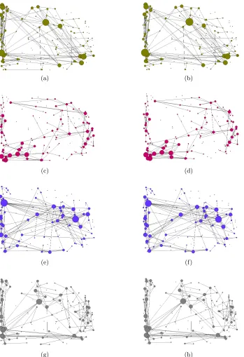
Using the aforementioned time series data, a 140×140 sample correlation matrix can be computed for each subject. Note that the number of samples is smaller than the number of variables and, therefore, the sample correlation matrix is not invertible. As a result, it is not possible to take the inverse of the sample correlation matrix for estimating a partial correlation matrix. The brain network being sought has n = 140 nodes (brain regions). In an effort to find a subgraph of this network as closely as possible to a spanning tree, we choose the regularization parameter λ in the graphical lasso algorithm and the level of thresholding in such a way that they both lead to graphs with n−1 = 139 edges. As illustrated in Figure 2, the similarity degree between the outcomes of these two techniques is above 90% for all twenty subjects. The outcomes of graphical lasso and thresholding obtained for 4 of these subjects are given in Figure 3 for illustration. Note that these graphs are not spanning trees as indented, which imply that graphical lasso and thresholding are able to obtain graphs with n−1 edges but they inevitably have cycles.
2 4 6 8 10 12 14 16 18 20 0
10 20 30 40 50 60 70 80 90 100
Subject
Similarity Degree (in Percentage)
Figure 2: The similarity degree of thresholding and graphical lasso for obtaining brain net-works of 20 subjects.
5. Case Study on Electrical Circuits
(a) (b)
(c) (d)
(e) (f)
(g) (h)
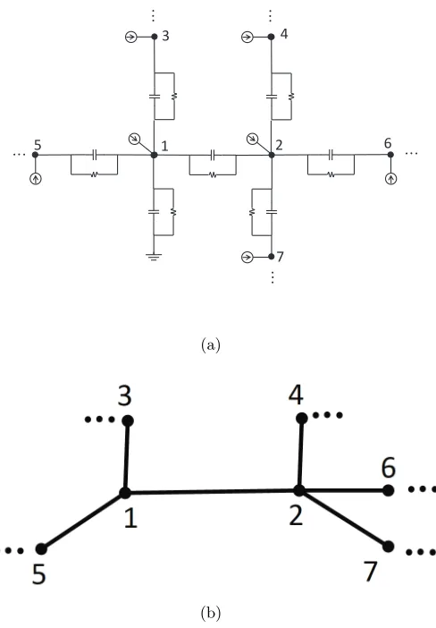
Σ∗ denote the “steady-state” covariance of the voltage measurements. It can be shown that Σ∗ = C−1, where C is the n×n capacitance matrix of the circuit (Sojoudi and Doyle, 2014). Note that the sparsity pattern of C is consistent with the topology of the circuit. Therefore, the inverse covariance matrix Σ−1∗ and the partial correlation matrix both have the same sparsity structure as the circuit. In other words, the partial correlation matrix unveils the physical connectivity of the circuit. Assuming that the circuit under study has a sparse structure, it can be concluded that
• Σ∗ is generically a dense matrix, due to being the inverse of the sparse matrix C.
• Σ−1∗ is sparse and its sparsity pattern conforms with the circuit topology.
1 2
3 4
5 6
7
(a)
(b)
Figure 4: a) An RC network with node 1 connected to the ground via a resistor and a capacitor, b) a graph representation of the RC network connectivity.
con-struct a sample covariance matrix as
Σ = 1
r
r
X
i=1
Vi(ti)Vi(ti)T (39)
whererdenotes the number of samples. Note that Σ converges to the population covariance Σ∗asr → ∞. Whenris finite, two possible scenarios arise: i) Σ is invertible but the inverse matrix needs to be thresholded to some level due to the error Σ∗−Σ, ii) Σ is not invertible and therefore alternative methods are needed to estimate the inverse matrix.
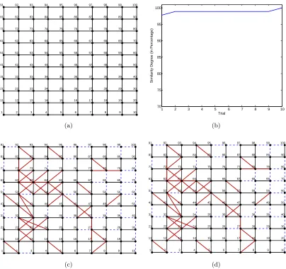
The above circuit model can be used to study the relationship between the thresholding and graphical lasso techniques. As an example, consider a mesh circuit with n = 100 nodes that are connected to one another through 180 links. The graphical model of this grid circuit is depicted in Figure 5(a). With no loss of generality, assume that Cij = −1 for all (i, j) ∈ E. Furthermore, suppose that nodes 2, 9, 22, 61 and 70 of the circuit are connected to the ground through parallel RC circuits with values equal to 0.1. For
r = 99 and 10 different trials, we have calculated the sample covariance matrices and applied the thresholding technique and graphical lasso to these matrices in order to recover networks with 180 edges. Note that since the number of samples is less than the number of variables, the sample partial correlations cannot be obtained through matrix inversion. The degree of similarity between graphical lasso and thresholding for these 10 trials are given in Figure 5(b). Figures 5(c) and 5(d) show the networks obtained from thresholding and graphical lasso for one of the trials. False positives are marked in red and false negatives are colored in blue. These two graphs have 178 edges in common (out of 180 edges), which indicates a high degree of similarity between the outcomes of the two techniques under study (to observe some of the few differences, one can inspect the existence of the edges (64,75) and (55,56) in these two graphs). We have repeated the above experiment on many circuit models beyond mesh networks and observed a very similar result.
6. Conclusions
0 2 4 6 8 10 12 0 2 4 6 8 10
1 2 3 4 5 6 7 8 9 10
11 12 13 14 15 16 17 18 19 20
21 22 23 24 25 26 27 28 29 30
31 32 33 34 35 36 37 38 39 40
41 42 43 44 45 46 47 48 49 50
51 52 53 54 55 56 57 58 59 60
61 62 63 64 65 66 67 68 69 70
71 72 73 74 75 76 77 78 79 80
81 82 83 84 85 86 87 88 89 90
91 92 93 94 95 96 97 98 99 100
(a)
1 2 3 4 5 6 7 8 9 10
70 75 80 85 90 95 100 Trial
Similarity Degree (in Percentage)
(b)
0 2 4 6 8 10 12
0 2 4 6 8 10 12 STH
1 2 3 4 5 6 7 8 9 10
11 12 13 14 15 16 17 18 19 20
21 22 23 24 25 26 27 28 29 30
31 32 33 34 35 36 37 38 39 40
41 42 43 44 45 46 47 48 49 50
51 52 53 54 55 56 57 58 59 60
61 62 63 64 65 66 67 68 69 70
71 72 73 74 75 76 77 78 79 80
81 82 83 84 85 86 87 88 89 90
91 92 93 94 95 96 97 98 99 100
(c) 00 2 4 6 8 10 12
2 4 6 8 10 12 S
GL: n−1
1 2 3 4 5 6 7 8 9 10
11 12 13 14 15 16 17 18 19 20
21 22 23 24 25 26 27 28 29 30
31 32 33 34 35 36 37 38 39 40
41 42 43 44 45 46 47 48 49 50
51 52 53 54 55 56 57 58 59 60
61 62 63 64 65 66 67 68 69 70
71 72 73 74 75 76 77 78 79 80
81 82 83 84 85 86 87 88 89 90
91 92 93 94 95 96 97 98 99 100
(d)
Figure 5: a) The mesh RC circuit studied in Section 5, b) the similarity degree of thresh-olding and graphical lasso for the mesh network over 10 trails, c) the network obtained from thresholding the sample correlation matrix for one trial, d) the network obtained from graphical lasso for the same trial used for Figure (c).
References
Onureena Banerjee, Laurent El Ghaoui, and Alexandre d’Aspremont. Model selection through sparse maximum likelihood estimation for multivariate Gaussian or binary data.
The Journal of Machine Learning Research, 9:485–516, 2008.
Alfred M Bruckstein, David L Donoho, and Michael Elad. From sparse solutions of systems of equations to sparse modeling of signals and images. SIAM review, 51(1):34–81, 2009.
Venkat Chandrasekaran, Pablo Parrilo, Alan S Willsky, et al. Latent variable graphical model selection via convex optimization. In 48th Annual Allerton Conference on Com-munication, Control, and Computing, pages 1610–1613, 2010.
Patrick Danaher, Pei Wang, and Daniela M Witten. The joint graphical lasso for inverse covariance estimation across multiple classes. Journal of the Royal Statistical Society: Series B (Statistical Methodology), 76(2):373–397, 2014.
Jianqing Fan and Jinchi Lv. A selective overview of variable selection in high dimensional feature space. Statistica Sinica, 20(1):101, 2010.
Salar Fattahi and Javad Lavaei. On the convexity of optimal decentralized control prob-lem and sparsity path. http: // www. ieor. berkeley. edu/ ~ lavaei/ SODC_ 2016. pdf, 2016.
Jerome Friedman, Trevor Hastie, and Robert Tibshirani. Sparse inverse covariance estima-tion with the graphical lasso. Biostatistics, 9(3):432–441, 2008.
Tom Goldstein and Stanley Osher. The Split Bregman method for L1-regularized problems.
SIAM Journal on Imaging Sciences, 2(2):323–343, 2009.
Dominique Guillot and Bala Rajaratnam. Retaining positive definiteness in thresholded matrices. http: // arxiv. org/ abs/ 1108. 3325, 2011.
Shuai Huang, Jing Li, Liang Sun, Jieping Ye, Adam Fleisher, Teresa Wu, Kewei Chen, Eric Reiman, Alzheimer’s Disease NeuroImaging Initiative, et al. Learning brain connectivity of alzheimer’s disease by sparse inverse covariance estimation. NeuroImage, 50(3):935– 949, 2010.
Ali Jalali, Pradeep D Ravikumar, Vishvas Vasuki, and Sujay Sanghavi. On learning dis-crete graphical models using group-sparse regularization. InInternational Conference on Artificial Intelligence and Statistics, pages 378–387, 2011.
Nicole Kr¨amer, Juliane Sch¨afer, and Anne-Laure Boulesteix. Regularized estimation of large-scale gene association networks using graphical Gaussian models. BMC bioinfor-matics, 10(1):384, 2009.
Han Liu, Kathryn Roeder, and Larry Wasserman. Stability approach to regularization se-lection (stars) for high dimensional graphical models. InAdvances in Neural Information Processing Systems, pages 1432–1440, 2010.
Rahul Mazumder and Trevor Hastie. Exact covariance thresholding into connected compo-nents for large-scale graphical lasso. The Journal of Machine Learning Research, 13(1): 781–794, 2012.
Nicolai Meinshausen and Bin Yu. Lasso-type recovery of sparse representations for high-dimensional data. The Annals of Statistics, pages 246–270, 2009.
Mark Schmidt, Alexandru Niculescu-Mizil, Kevin Murphy, et al. Learning graphical model structure using L1-regularization paths. InAAAI, volume 7, pages 1278–1283, 2007.
Somayeh Sojoudi. Graphical lasso and thresholding: Conditions for equivalence. http: // www. somayehsojoudi. com/ GL_ Versus_ TH2. pdf, 2016.
Somayeh Sojoudi and John Doyle. Study of the brain functional network using synthetic data. In52nd Annual Allerton Conference on Communication, Control, and Computing, pages 350–357, 2014.
Robert Tibshirani. Regression shrinkage and selection via the lasso. Journal of the Royal Statistical Society. Series B (Methodological), pages 267–288, 1996.
Petra E V´ertes, Aaron F Alexander-Bloch, Nitin Gogtay, Jay N Giedd, Judith L Rapoport, and Edward T Bullmore. Simple models of human brain functional networks.Proceedings of the National Academy of Sciences, 109(15):5868–5873, 2012.
Daniela M Witten, Jerome H Friedman, and Noah Simon. New insights and faster compu-tations for the graphical lasso. Journal of Computational and Graphical Statistics, 20(4): 892–900, 2011.
John Wright, Allen Yang, Arvind Ganesh, Shankar Sastry, and Yi Ma. Robust face recog-nition via sparse representation. IEEE Transactions on Pattern Analysis and Machine Intelligence, 31(2):210–227, 2009.
Ming Yuan and Yi Lin. Model selection and estimation in the Gaussian graphical model.
Biometrika, 94(1):19–35, 2007.