In Search of Coherence and Consensus:
Measuring the Interpretability of Statistical Topics
Fred Morstatter [email protected]
University of Southern California Information Sciences Institute 4676 Admiralty Way Ste. 1001 Marina Del Rey, CA 90292
Huan Liu [email protected]
Arizona State University 699 S. Mill Ave
Tempe, AZ 85283
Editor:David Blei
Abstract
Topic modeling is an important tool in natural language processing. Topic models provide two forms of output. The first is a predictive model. This type of model has the ability to predict unseen documents (e.g., their categories). When topic models are used in this way, there are ample measures to assess their performance. The second output of these models is the topics themselves. Topics are lists of keywords that describe the top words pertaining to each topic. Often, these lists of keywords are presented to a human subject who then assesses the meaning of the topic, which is ultimately subjective. One of the fundamental problems of topic models lies in assessing the quality of the topics from the perspective of human interpretability. Naturally, human subjects need to be employed to evaluate interpretability of a topic. Lately, crowdsourcing approaches are widely used to serve the role of human subjects in evaluation. In this work we study measures of interpretability and propose to measure topic interpretability from two perspectives: topic coherence and topic consensus. We start with an existing measure for topic coherence—model precision. It evaluates coherence of a topic by introducing an intruded word and measuring how well a human subject or a crowdsourcing approach could identify the intruded word: if it is easy to identify, the topic is coherent. We then investigate how we can measure coherence comprehensively by examining dimensions of topic coherence. For the second perspective of topic interpretability, we suggest topic consensus that measures how well the results of a crowdsourcing approach matches those given categories of topics. Good topics should lead to good categories, thus, high topic consensus. Therefore, if there is low topic consensus in terms of categories, topics could be of low interpretability. We then further discuss how topic coherence and topic consensus assess different aspects of topic interpretability and hope that this work can pave way for comprehensive measures of topic interpretability.
1. Introduction
Understanding natural language is one of the cornerstones of artificial intelligence research. Researchers can usually rely on text to give them signal for their specific problem. Text has been used to greatly aid artificial intelligence tasks such as opinion mining (Pang and
c
Lee, 2008; Tumasjan et al., 2010), and user home location detection (Mahmud et al., 2012), and to find users in crisis situations (Morstatter et al., 2014). Topic modeling is one of the prominent text analysis techniques. Formally, topics are probability distributions over the words, but usually researchers treat them as lists of the most probable keywords. This process is akin to organizing newspaper articles by the “section” in which they appear, and simultaneously ranking words for that section. Topic models have been widely used for many tasks in social media research, such as using text to discover topics of discussion in crisis scenarios (Kireyev et al., 2009), event detection and analysis (Hu et al., 2012), and finding a Twitter user’s home location (Eisenstein et al., 2010).
Topic modeling describes a family of approaches which work toward the above task. Latent Dirichlet Allocation (Blei et al., 2003), commonly known as LDA, is one example of a very popular topic model. LDA, and models like it, are used from two perspectives. The first is as a predictive model. When LDA is used in this way, the application is clear: there are many existing measures to assess the predictive performance. The other main use of LDA is to describe the dataset. The topics it learns are read by humans for them to get a better picture of the underlying themes in the dataset. When used this way, the topic distributions are manually inspected in many studies to show that some underlying pattern exists in the corpus. The meaning behind these topics is often interpreted by the individual who builds the model, and topics are often given a title or name to reflect their understanding of the underlying meaning of the topics. One key concern with topic models
lies with how well human beings can actually understand the topics, or the problem oftopic
interpretability. It may be true that when presented with a group of words a human subject will always be able to assign some meaning. In this work, we question if we can tap on a group of human subjects or crowdsourcing in search of measures for topic interpretability.
We focus on assessing the interpretability of topics from two perspectives: coherence,
and consensus. Coherence measures how semantically close the top words of a topic are. Consensus measures how well the results of a crowdsourcing approach or generated by a group of human subjects match those given categories of topics.
The main contributions of this work are:
• We elaborate the need for measuringtopic coherence, a novel dimension for measuring
the semantic quality of topics. Based on this dimension, we propose “Model Precision Choose Two”, a measure to comprehensively estimate how well a topic’s top words are related to each other;
• We propose a topic consensus measure that estimates how well a statistical topic
represents an underlying category of text in the corpus; and
• We demonstrate how these measures complement the existing framework and show
how the results of these measures can help to further discover interpretable topics by a topic model.
2. Related Work
widely applied to social media data. In the context of disaster-related tweets, Kireyev et al. (2009) tries to find disaster-related tweets, modeling two types of topics: informational and emotional. Joseph et al. (2012) studies the relation between users’ posts and their geolocation. Several works (Yin et al., 2011; Hong et al., 2012; Pozdnoukhov and Kaiser, 2011) focus on identifying topics in geographical Twitter datasets, looking for topics that pertain to things such as local concerts and periods of mass unrest. Topic modeling was also used to find indication of bias in Twitter streams (Morstatter et al., 2013). Topic models exist have been developed to meet the unique needs of web data (Lin et al., 2014).
With such a wide acceptance, it is important that the topics produced by topic models are evaluated. Approaches to evaluating topic models follow two main avenues: evaluating the predictive performance of the model, and evaluating its interpretability. While we only focus on the latter in this work, we will cover the related work in the area of assessing the predictability before moving on to discuss the evaluation of interpretability.
2.1 Evaluating the Predictive Power of Topic Models
In the most general case, topic models are run over large corpora of data that do not contain a “ground truth” definition of the topics in the text. Because of this, we cannot apply supervised machine learning measures such as accuracy, precision, and recall to the task. Instead, the most often used measure for the predictive performance of topic models is “perplexity” (Jelinek et al., 1977; Jurafsky and Martin, 2000), which measures how well the topics match a set of held-out documents (Blei et al., 2003; Griffiths and Steyvers, 2004; Kawamae, 2016; Asuncion et al., 2009). Perplexity is defined as:
perp(q, x) = 2− 1
|x|
P|x|
i=1log2q(xi)
, (1)
whereq is the model we are testing, andx is the set of held-out documents. The intuition
is that we are measuring how perplexed, or surprised, the model is. If the documents in
x have a high probability of occurring, then the summation in the exponent will have a
greater value, and thus the overall perplexity score will have a lower value.
Some specialized topic models can leverage ground truth labels. One such case is “La-beled LDA” (Ramage et al., 2009a), which is a different approach that takes labels into account when building the model. When evaluating its performance, traditional measures
for supervised machine learning are applied such as F1 (Frakes and Baeza-Yates, 1992),
which is calculated as:
F1=
2πρ
π+ρ, (2)
whereπ = T PT P+F P is the precision andρ= T PT P+F N is the recall. Obtaining “true positives”, “false positives”, “true negatives”, and “false negatives” requires data with ground truth, which is why we could not apply it when no labels are available.
2.2 Evaluating the Interpretability of Topic Models
thought. The first school of thought is ad-hoc, where researchers manually read topics in order to judge their quality. In the second, researchers take a more principled approach, employing measures that can judge the quality of topics in a more automated manner. In the subsequent subsections, we provide more details regarding each approach and the related work that employs it.
2.2.1 Eyeballing
The most common approach to assessing the quality of topics is the “eyeballing” approach, where topics are inspected carefully and manually assigned a label. After the topics are read, a “title” is assigned to each one based upon the top keywords in the text. In Grimmer and Stewart (2013), the authors manually label topics based upon the top words in the topic. These manual topic labels are supplemented with automatic labeling approaches such as Aletras and Stevenson (2014); Lau et al. (2011); Maiya et al. (2013); Mao et al. (2012), however the final call is made by a human. In other work, topic models were verified on scientific corpora to show that the topics that were produced by the model made sense (Blei et al., 2003; Griffiths and Steyvers, 2004). By displaying the top words from the topics to the reader, they make the case that the topics they find are of high quality. In the context of related tweets, Kireyev et al. (2009) try to find disaster-related tweets, labeling two types of topics: informational and emotional. This was done by interpreting a visualization of the topic clusters and manually assigning meaning to the topic groups. Other forms of visualization have been proposed to identify interpretable topics, such as that proposed in Le and Lauw (2016) where the authors show topics in a low-dimensional embedding. Another visualization approach is proposed in Sievert and Shirley (2014), where the authors show topics, their top words, and the size of the topic to the user to help them differentiate interpretable topics. Similarly, Hu et al. (2014) created an approach to iteratively add constraints to generate better topics.
The manual labeling of topics goes beyond mere text. For example, Schmidt (2012)
uses LDA to cluster 1820’s ship voyages. By treating trips as documents and nightly
latitude/longitude checkins as words, the authors generate topics based upon these trips. Using manual inspection of topics, the authors are able to label topics as “trading” and “whaling” topics, amongst others. Other works focus on identifying topics in geographical Twitter datasets, looking for topics that pertain to things such as local concerts and periods of mass unrest (Yin et al., 2011; Hong et al., 2012).
While the manual inspection of topics is often used for topic labeling, it can also be used for topic filtering. In Kumar et al. (2013), the authors employ subject-matter experts to label the topics for them. In this case the authors had the labelers mark the topics as “relevant” to their study, or “not relevant”. Ultimately those topics that were not deemed relevant were removed.
0 20 40 60 80 100 120 Female Male (a) Sex 0 10 20 30 40 50 60 70 80
18 - 25
26 - 35
36 - 45
46 - 55 56 - 65
> 65 (b) Age 0 10 20 30 40 50 60 70 80
No High School
High School Some College Bachelors Masters PhD (c) Education 0 20 40 60 80 100 120 140 160 180 English Other Hindi Spanish Mandarin Russian
(d) First Language
0 20 40 60 80 100 120 140 160 USA India
Canada Mexico China Turkey Armenia Croatia Russia Spain
(e) Origin Country
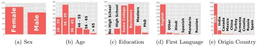
Figure 1: Demographic breakdown of the Turkers who participated.
2.2.2 Principled Evaluation of Topic Interpretability
This method of assessing topic quality employs formal approaches and measures to assess the interpretability of statistical topics, generally through crowdsourcing. While aggregat-ing the results of crowdsourced tasks is challengaggregat-ing, some work has focused on leveragaggregat-ing crowdsourcing to assess human interpretability (Zhou et al., 2014). Chang et al. (2009) pro-posed the first such framework for topic models in which a hybrid approach was employed. This approach focuses on crowdsourcing in order to assess topic interpretability. The results of the crowd are then aggregated through different measures to give a “score”, which is a numerical value indicating the topic’s interpretability. While not truly automated, it pro-vides a reproducible framework that can be used by researchers to perform this assessment. In their paper, the authors focus on two main validation schemes for topic models: “Word Intrusion” which studies the top words within a topic by discovering how well participants can identify a word that does not belong. They also introduce “Topic Intrusion”, which studies how well the topic probabilities for a document match a human’s understanding
of this document by showing three highly-probably topics, and one improbable topic, and
asking the worker to select the “intruder”.
Chang’s influential paper provided the groundwork for a principled study of topic in-terpretability. Subsequent work aimed to provide automated approaches to replace the Turkers. Lau et al. (Lau et al., 2014) went about this by building heuristics to guess the actions of the workers. They provide an algorithm that will guess which answer a crowd-sourced worker will choose when presented in an Human Intelligence Task (HIT). Other
investigations into this measure include Roder et al. (R¨oder et al., 2015), who
automati-cally explore the space of possible weights applied to existing interpretability measures and aggregation functions to find the measure that best approximates model precision.
2.3 Crowdsourcing Approaches to Evaluation
The crowdsourced experiments carried out in this work were performed using Amazon’s
Mechanical Turk1 platform. Mechanical Turk is a crowdsourcing platform that allows
re-questers to coordinate Human Intelligence Tasks (HITs) to be solved by Turkers. The formulation of each HIT will be described in the corresponding section for each experiment. In all cases, each HIT was solved 8 times to overcome issues that arise from using non-expert annotators (Snow et al., 2008).
Document 1:
board presenta,on massive american beef domes,c Document 2: basketball hall fame Document 3:
...
LDA
K
Topic 1 Topic 2 ... Topic K
Document1 0.2 0.1 0.01
Document2 0.7 0.02 0.1
...
Documentn 0.1 0.3 0.02
Topic 1: season 2.0% game 1.8% home 1.5% start 1.2% hit 1.0%
Topic 2: percent 3.3% market 1.6% fell 1.3% shares 1.2% u.s. 1.2%
Topic K: film 1.9% series 1.1% director 0.8% tv 0.8% movie 0.8%
...
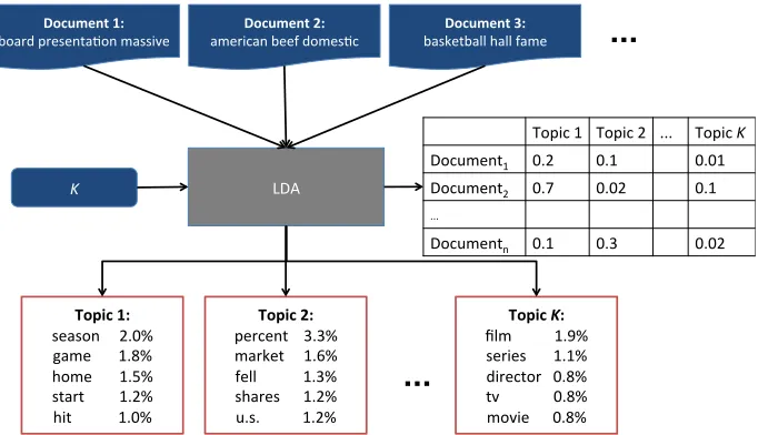
Figure 2: An overview of the LDA process. Each document is presented as a bag of words
along withK, the number of topics the LDA operator wishes to discover. Two outputs are
provided: the topics (on the bottom), and the document-topic associations (on the right).
In this paper we experiment with three measures that rely on crowdsourcing platforms like Amazon’s Mechanical Turk. In order to ensure the reliability, as well as to account for noise in the results, it is important to have a basic understanding of the userbase solving the HITs we create. Prior to solving any HITs, we require the Turker to fill out a demographic survey. The demographic survey consists of five questions about the Turker’s background: their sex, age, first language, country of origin, and highest level of education achieved. The demographic makeup of our Turkers can be seen in Figure 1. Figures 1(d) and 1(e) reveal a strong skew towards American Turkers who speak English as their first language. This could be partly attributed to a recent change in the Mechanical Turk terms of service
that requires Turkers to provide their Social Security Number2 in order to solve HITs on
the site. Regardless, this allows us to go forward knowing that the participants are largely English speakers, and we cannot attribute poor performance in our analysis to a poor grasp of English.
This exercise in understanding the demographic makeup of our Turkers is done to give us a sense of the expected demographic makeup in future studies. We do not delete any Turkers who are non-native speakers. Instead, we investigate a Turkers’ ability to solve our HITs based upon their performance at the “sanity” questions, the easiest HITs to solve in our set. These would be “control questions” to differentiate genuine workers (Liu et al., 2013). Initially, we planned to delete users who missed over 25% of these questions. Fortunately, no user fell below this threshold, and consequently no user was deleted from our study.
3. Topic Modeling
Topic modeling refers to a family of models that seek to discover abstract “topics” that occur within a corpus (Blei, 2012). Different approaches have been proposed for this task. For example, one of the first topic models was PLSA (Hofmann, 1999). LDA (Blei et al., 2003) built on this by adding a Dirichlet prior to the document-topic distribution. Many ap-proaches have also been proposed for this task such as Hierarchical Dirichlet Processes (Teh et al., 2006), Correlated Topic Models (Blei and Lafferty, 2006), and Pachinko Allocation (Li and McCallum, 2006). While these are more recent than LDA, LDA is the most widely used topic modeling approach.
3.1 Latent Dirichlet Allocation
The goal of topic modeling is to learn “topics” from a large corpus of text. In LDA, each topic is a probability distribution over the entire vocabulary of the corpus. While each topic contains every word, the probabilities assigned to the word vary by topic. Furthermore, the model learns an association for each document over each of the topics. In other words, each document is described as a probability distribution over all of the topics in the corpus.
Formally, LDA takes two inputs:3 A bag-of-words corpus containing ddocuments and
a vocabulary of sizev, and a scalar valueK, which indicates the number of topics that the
model will learn. LDA then outputs a model,m. The model, m, consists of two matrices:
1. A T opic×V ocabulary matrix, Tm ∈ RK×v. This is the matrix of topics that are
learned by the model. Tmi,j is the association of wordj with topic i.
2. ADocument×T opicmatrix,Dm∈
Rd×K, with entryDmi,jrepresenting the probability
that document iis generated by topic j.
This is the fundamental input and output of the model, and can be seen in Figure 2. The model can be trained either through expectation maximization (Blei et al., 2003), or through Gibbs sampling (Griffiths and Steyvers, 2004). In this work we use the Mallet toolkit (McCallum, 2002), which uses the latter strategy to learn the parameters.
Beyond the notation, Figure 2 more clearly articulates the two schools of thought out-lined in Section 2. When a researcher employs the “eyeballing” approach described in Sec-tion 2.2.1, what they are doing is having a human read the top words in the topic (depicted at the bottom of the figure) and divining a meaning for the topic. For example, a researcher may read the top words of “Topic 1” in Figure 2 and call it a “sports topic”. While this ultimately may be an appropriate guess, there is no existing measure to determine the how well the definition fits the topic.
Principled evaluation, the second school of thought outlined in Section 2.2.2, consists of applying a standard framework to the practice of assessing topic quality. In (Chang et al., 2009), the authors propose a hybrid framework to assess topic quality, while (Mimno et al., 2011) propose a solution to do it automatically. The thrust of this work is to extend the existing principled framework in order to assess new dimensions of topic quality.
Going forward we will reproduce “Model Precision”, one of the measures introduced in (Chang et al., 2009). Next, we will provide two new measures which can extend the
isting framework and show how the insights they provide compare to the existing solution. The measures we propose are also hybrid, meaning that they depend on crowdsourcing to obtain their results. We note that while useful, this has major implications for reproducibil-ity. These experiments require ample time and money in order to run, making it intractable for many researchers. Thus, we experiment with automated measures that can replace the effort performed by the crowdsourced workers.
3.2 Data
We generate topics from LDA using two datasets. First, we use a dataset of scientific abstracts from the European Research Council. The text in these documents is of high quality, written by scientists who wish to argue their case in order to secure funding for their research. It is possible that topical misunderstanding can stem from a lack of understanding of the crowdsourced workers, who are not necessarily trained to understand scientific text. To complement this dataset, we use a large corpus of news articles curated by Yahoo News. We introduce both of these datasets in the subsequent sections.
3.2.1 Scientific Abstracts
The first text corpus focused upon in this study consists of 4,351 abstracts of accepted
research proposals to the European Research Council.4 In the first 7 years of its existence,
the European Research Council (ERC) has funded approximately 4,500 projects, 4,351 of which are used in this study. Abstracts are limited to 2,000 characters, and when a researcher submits an abstract, they are required to select one of the three scientific domains their research fits into: Life Sciences (LS), Physical Sciences (PE), or Social Sciences and Humanities (SH). These labels will be used in the crowdsourced measure we propose later. Mapping scientific research areas has become of growing interest to scientists, policy-makers, funding agencies and industry. Traditional bibliometric data analyses such as co-citation analysis supply us with basic tools to map research fields. However, Social Sciences and Humanities (SH) are especially difficult to map and to survey, since the fields and disci-plines are embedded in diverse and often diverging epistemic cultures. Some are specifically bound to local contexts, languages and terminologies, and the SH domain lacks coherent referencing bodies or citation indices, and dictionaries (Mayer and Pfeffer, 2014). Further-more, SH terminology is often hard to identify as it resembles everyday speech. Innovative semantic technologies such as topic modeling promise alternative approaches to mapping SH, but the basic question here is: how interpretable are they and how can their results be evaluated in a systematic way? This raises further questions into the interpretability of the LDA topics we study in this paper.
The abstracts used in this research were accepted between 2007–2013, written in English,
and classified by the authors5 into one of the three main ERC domains. The first column of
Table 1 shows some statistics of the corpus. The aim of each abstract is to provide a clear understanding of the objectives and methods to achieve them. Abstracts are also used to find reviewers or match authors to panels.
Table 1: Properties of the European Research Council accepted abstracts and Yahoo News corpora. The values for each category represent the number of documents in the category.
Property ERC Data Yahoo News Data
Documents 4,351 258,919
Tokens 649,651 6,888,693
Types 10,016 214,957
Category 1 LS: 1,573 S: 88,934
Category 2 PE: 1,964 B: 90,159
Category 3 SH: 814 E: 79,826
3.2.2 News Data
The second text corpus used in this work consists of 258,919 news articles indexed by
Yahoo News.6 Yahoo News maintains a corpus of every news article published on its site
between 2015-02-01 and 2015-06-03.7 Similar to newspapers, these articles are tagged with
a “section”, which corresponds to a categorization. In this study, we select articles from three such categories: Sports (S), Business (B), and Entertainment (E).
The rationale for choosing this dataset is that discovering the topics of a corpus is very similar to automatically discovering the “sections” of a newspaper. When individuals read the top words of a topic, they often assign meanings to the topics, which could correspond to the types of categories seen in newspapers (Grimmer and Stewart, 2013). We employ this corpus because it can give us exactly this mapping, and, in the case of one of our measures, tells us exactly how well these topic understandings map onto the true distribution of the topic. Another important distinction of this dataset is that it consists of text that is meant to be read by everyone.
All of the articles in this corpus were written between February 1st, 2015 and June 3rd, 2015, in English, and classified by Yahoo into one of the three aforementioned categories. The summary statistics of our corpus can be seen in the second column of Table 1.
3.3 Extracting Topics from Text
We apply LDA to extract topics from the text. We run LDA on each dataset four times,
with K = 10,25,50,100, yielding a total of 185 ERC topics, and 185 Yahoo News topics.
All LDA runs were carried out using the Mallet toolkit (McCallum, 2002). Before running LDA, we stripped the case of all words and removed stopwords according to the MySQL
stopwords list.8 Tokenization was performed using Mallet’s preprocessing framework,
us-ing a special regular expression which preserves punctuation within words.9 This allows
for URLs, contractions, and possessives to be preserved. In all experiments, we fix the
hyperparameter values to α= 5.0 andβ = 0.01.
6.https://www.yahoo.com/news/
7.https://webscope.sandbox.yahoo.com/catalog.php?datatype=r&did=75 8.http://www.ranks.nl/stopwords
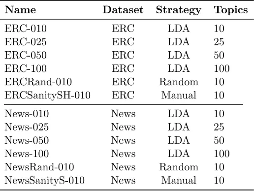
Table 2: The LDA models generated for this study. These indicate the different values of
“m” used throughout the experiments, e.g.in Equation 3.
Name Dataset Strategy Topics
ERC-010 ERC LDA 10
ERC-025 ERC LDA 25
ERC-050 ERC LDA 50
ERC-100 ERC LDA 100
ERCRand-010 ERC Random 10
ERCSanitySH-010 ERC Manual 10
News-010 News LDA 10
News-025 News LDA 25
News-050 News LDA 50
News-100 News LDA 100
NewsRand-010 News Random 10
NewsSanityS-010 News Manual 10
In addition to the LDA runs, we extract two additional topic groups from each corpus. This is done with the intent of giving some controls to understand the bounds of the topic
measures. The first is a set ofrandom topics. To generate these topics, we weight the words
by their frequency in the corpus and randomly draw words from this distribution. These topics have a roughly equal mixture of the three categories in the corpus they represent.
To complement our random topics, we also create a set of “sanity” topics. These topics are handpicked to be a clear representation of one of the categories. In the ERC corpus, we calculate each word’s probability of occurring in a SH, LS, or PE document. We then select
words that occur most (>95% of the time) in the SH category. Furthermore, we ensure that
these words occur in fewer than<5% of the documents from the other two categories. The
intention behind these topics is that they provide a strictly pure representation of the SH category, and should provide as a useful sanity check of the Turker’s labeling abilities. The same process is repeated with the Yahoo News data, by selecting topics similarly skewed towards the S category. These topics lie in contrast to the random topics in that they are strongly skewed to represent a single group.
In both cases of random and sanity topics, these topics are unlike traditional LDA topics,
containing only a set of 5 words. We use both of these auxiliary topic sets for validation
of the results obtained using the LDA topics. Table 2 shows an overview of all of the topic sets generated for this study.
0.00 0.25 0.50 0.75 1.00
ERC−010 ERC−025 ERC−050 ERC−100 ERCRand−010
ERCSanitySH−010 Topic Group
Model Precision
MP − ERC
(a) ERC Data
0.00 0.25 0.50 0.75 1.00
News−010News−025News−050News−100
NewsRand−010NewsSanityS−010 Topic Group
Model Precision
MP − News
(b) Yahoo News Data
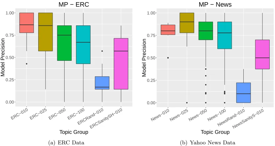
Figure 3: Results of “Model Precision” task on the topic sets from the two datasets. The horizontal bar represents the median, and the dots represent outliers.
4. Topic Coherence
One definition of coherence is “the quality or state of systematic or logical connection
or consistency”.10 When a topic is a set of words, its coherence is about the relationships
among the words. Since each individual can have their opinion of coherence, a crowdsourcing approach is used to obtain a group’s feedback. This transforms an individual’s opinion to a distribution of collective opinions. We first introduce Chang et al.’s ingenious measure of coherence.
4.1 Model Precision — A Measure of Coherence
Model Precision, introduced by (Chang et al., 2009), is a widely used measure of the “co-herence” of an individual topic. It measures the distinctness of a randomly-inserted word into the top five words of a topic. The intuition is that if humans are consistently able to identify the randomly-inserted word, then the topic is more coherent because the intruded word is clearly distinct from the other 5 words. On the other hand, if the humans cannot consistently choose this randomly-inserted word, then the top 5 words of the topic are likely not coherent. This is because the humans are conflating the definition of the top words in the topic with a word that is far away.
For each topic, we show the Turker the top 5 most probable words from the topic’s
probability distribution along with one of theleast probable words in the distribution. We
call this word the “intruded” word. To prevent rare words from being selected as the
intruder, we ensure that it is also among the top 5 words from another topic. We then ask the Turker to select the word that they think is the intruded word. Model precision is the number of times a Turker was able to guess the intruded word divided by the number of times the HIT was solved, formally:
M Pkm= 1
|smk|
|smk|
X
i=1
1(gkm=smk,i), (3)
whereM Pkm is the model precision of thek-th topic from modelm,gmk is the ground-truth
intruded word for topic k,smk is the vector of choices made by Turkers on topick, and 1(·)
is the indicator function which yields 1 ifgm
k =smk,i, and 0 otherwise.
The results of this measure on both of our datasets are shown in Figure 3. These figures show boxplots which depict the performance of the topics against this measure. Following traditional boxplot visualization techniques (Wickham and Stryjewski, 2011), the dark horizontal line in the middle of the box is the median, and the lower stem, lower box, upper box, and upper steam each account for 25% of the data. Dots represent topics
determined to be outliers by a rule.11
We expect that the results would put the interpretability of the LDA topics somewhere in between the random and sanity topics. They should perform better than the random topics, as these are designed to be uninterpretable. Furthermore, our LDA topics should underperform when compared with the sanity topics, which are designed specifically to be highly interpretable. In fact, the results only partially back up this intuition. While the random topics do in fact perform very poorly, the LDA topics actually outperform the sanity topics. This is likely due to the homogeneity of the topics and the words from their
vocabulary. When all of the choices are “SH” words in the ERC corpus, or “S” words in
the News corpus, it is quite likely that the human workers will be confused.
While comparing the distributions of the results may shed light on the broad strokes, the outliers may also provide insight about the results of the experiments. For example, in
bothK= 10 cases, we see one outlier, indicating one underperforming topic. In the random
topic set on the ERC data, we see one topic overperforming, doing much better than the
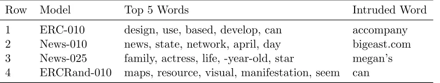
rest of the topics and even scoring near the median of the sanity topics. The four HITs are shown in Table 3. These results illuminate the issue of how these topics became outliers: the intruding word. In the bad topic modeling topics (rows 1, 2, and 3), the topics perform badly because they are not coherent. The words spread over many different concepts, and it is difficult to decipher the meaning. On the other hand the random topic which should have done badly (row 4) actually outperforms the rest of the topic set. Turkers coalesced around “can”, and “seem” as the intruded words. Since these are randomly-generated topics, any word among the 6 could be considered “intruded”, but only one answer is selected as correct from the setup of our HITs. It just so happened that “can” was the selected word, leading this topic to have an uncharacteristically high score.
These results may also give some inclination about how to use this measure. In fact,
there are any number of ways to use these results. For example, if we setK = 10, we will get
10 topics from the dataset. On large corpora like those used here, we should expect these
10 topics to be very generic, encompassing major themes of the text. WithK = 100 topics,
Table 3: Outlier topics from Model Precision.
Row Model Top 5 Words Intruded Word
1 ERC-010 design, use, based, develop, can accompany
2 News-010 news, state, network, april, day bigeast.com
3 News-025 family, actress, life, -year-old, star megan’s
4 ERCRand-010 maps, resource, visual, manifestation, seem can
we may also get generic topics, and additionally we are more likely to get fine-grained topics
that discuss more specific issues. For example, if in theK = 10 case we get one “politics”
topic, we may expect to get topics pertaining to specific candidates, issues, and localities
in the K = 100 case. Interpretability measures can help to shed light on which topics are
understandable by humans, and may give an indication of which topic model, or which topics within a model are the most interpretable.
In the following, we first examine what is not assessed by model precision in terms of coherence, and suggest the need for a new measure that can complement model precision for comprehensive measure of coherence.
4.2 A Missing Dimension of Model Precision
Model Precision works by asking the user to choose the word that does not fit within the rest of the set. We are measuring the top words in the topic by comparing them to an outlier. While this method is very useful for this task, it does not measure the coherence within the top words for the topic. This is because a good topic should have top words that are semantically close to each other, an aspect of topic quality which is not accounted for by Model Precision.
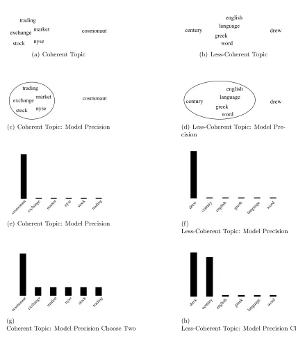
A diagram illustrating this phenomenon is shown in Figure 4. In Figure 4(a), we see a coherent topic. This topic is coherent because all 5 of the top words are close together, while the intruded word is far away. In Figure 4(b) we see a topic that is less coherent because the fifth word lies at a distance from the first four. In both cases, Model Precision gives us the intruder word in the topic, as seen in Figures 4(c), and 4(d). While this is the desired performance of Model Precision, it leaves us with no understanding of the coherence of the top words of the topic. Results are masked by the outlier, and do not give information about the intra-cluster distance, or coherence of the topic.
In light of this, we look for a way to separate topics not just by their distance from an outlier, but also by the distance within the top words in the topic. The next section of this paper investigates a method which can measure not just the intruder word, but also the coherence of the top words in the topic. In this way we separate topics such as those shown in Figure 4 based on the coherence of their top words.
4.3 Model Precision Choose Two — Another Dimension of Coherence
trading market exchange
stock nyse
cosmonaut
(a) Coherent Topic
language english
word greek
century drew
(b) Less-Coherent Topic
trading market exchange
stock nyse
cosmonaut
(c) Coherent Topic: Model Precision
language english
word greek
century drew
(d) Less-Coherent Topic: Model Pre-cision tradi ng marke t excha
nge nyse stock
cosm onaut
(e) Coherent Topic: Model Precision
langua ge engl ish word greek cent ury drew (f)
Less-Coherent Topic: Model Precision
excha nge
cosm
onaut marke trading t
stoc k nyse
(g)
Coherent Topic: Model Precision Choose Two
langua ge engl ish word greek cent ury drew (h)
Less-Coherent Topic: Model Precision Choose Two
Figure 4: Comparison between Model Precision, and Model Precision Choose Two for two real topics from the Yahoo News corpus. In Figures 4(g) and 4(h), the height of the bars represents the number of times the word was selected in the crowdsourced experiments. Model Precision Choose Two can distinguish the less-coherent topic.
inject one low-probability word. The key difference is that we ask the Turker to selecttwo
intruded words among the six.
quality clear. In a coherent topic the Turkers won’t be able to distinguish a second word as all of the words will seem similar. A graphical representation of this phenomenon is shown in Figure 4(g). In the case of an incoherent, a strong “second-place” contender will emerge as the Turkers identify a 2nd intruder word, as in Figure 4(h).
4.3.1 Experimental Setup
To perform this experiment, we injectone low-probability word for each topic, and we ask
the Turkers to selecttwo words that do not fit within the group. We show the six words to
the Turker in random order with the following prompt:
You will be shown six words. Four words belong together, and two of them do not. Choose two words that donotbelong in the group.
Coherent topics will cause the Turkers’ responses regarding the second intruded word to be unpredictable. Thus, our measure of the goodness of the topic should be the pre-dictability of the Turkers’ second choice. We propose a new measure called “Model Precision Choose Two” to measure this. Model Precision Choose Two (MPCT) measures this spread
as the peakedness of the probability distribution. We defineM P CTm
k for topickon model
m as:
M P CTkm=H pturk(wk,m1), ..., pturk(wmk,5)
, (4)
whereH(·) is the Shannon entropy (Lin, 1991), wm
k is the vector of the top words in topic
k generated by model m, and pturk(wmk,i) is the probability that a Turker selects wmk,i.
This measures the strength of the second-place candidate, with higher values indicating a smoother, more even distribution, and lower values indicating Turkers gravitation towards a second word.
The intuition behind choosing entropy is that it will measure the unpredictability in the Turker selections. That is, if the Turkers are confused about which second word to choose, then their answers will be scattered amongst the remaining five words. As a result, the
entropy will be high. Conversely, if the second word is obvious, the Turkers will begin to
congregate around that second choice, meaning that their answers will be focused. As a
result, the entropy will be low. Because entropy is able to measure the confusion of the
Turkers responses about the second word, we use it directly in the design of our measure.
4.3.2 Results and Discussion of Model Precision Choose Two
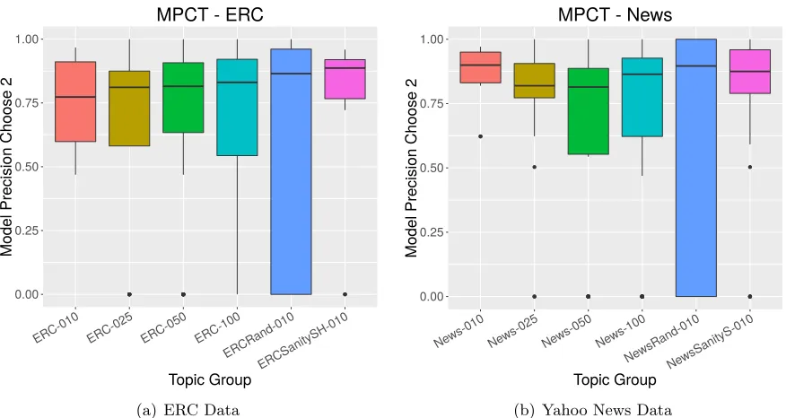
The results of this experiment on both corpora are shown in Figure 5. The box plots show the distribution of the results across all of the topics in each topic group. These results illustrate the differences between the two datasets in terms of both performance as well as
the appropriate value ofK, the number of topics, to maximize the performance. In the ERC
data a larger value ofK consistently improved our results, while with the News dataset we
achieved better results with a largerK.
The results of the MPCT experiments showed how to compute this measure on a topic set. While this new measure elicits another dimension of the topics, their coherence, they alone to not provide the whole picture of what makes a good topic.
0.00 0.25 0.50 0.75 1.00
ERC-010 ERC-025 ERC-050 ERC-100
ERCR
and-010
ERCSanitySH-010
Topic Group
Model Pr
ecision Choose 2
MPCT - ERC
(a) ERC Data
0.00 0.25 0.50 0.75 1.00
News-010 News-025 News-050News-100
NewsRand-010NewsSanityS-010
Topic Group
Model Pr
ecision Choose 2
MPCT - News
(b) Yahoo News Data
Figure 5: Results of “Model Precision Choose Two” on the topic sets from the two datasets. The figures are presented as before, with the horizontal bar indicating the median, and the dots representing outliers.
topics is also very high. It is easy to see why this occurs: in both very good and in very
bad topic groups, the Turker has a difficult time choosing any second choice intruder, which drives the MPCT score up. Because of this, we need to combine these results with model precision in order to get a good understanding of the topic quality.
To better compare the results, we compare a case-by-case basis in Figure 6. Both yield similar results which show interesting properties about the dataset. First, Figures 6(c) and 6(f) confirm our hypothesis that random topics can have a high MPCT. However, these lousy topics all have a low MP score. Curiously, though, we see in Figures 6(a) and 6(d) show another interesting pattern: that it is possible for topics to have a high MP and a low MPCT.
To better demonstrate what these values mean for a topic, we show several topics along-side their MP and MPCT scores in Table 4. We show topics of varying quality from the perspective of both measures we introduce. By reading the topics, we can make several observations. First, row 1 and 2 have both high MP and high MPCT. Contrast these topics with rows 3 and 4 which have a high MP score, yet a low MPCT score. When we look at the intruded word in rows 1–4, they all seem equally “distant”, however in rows 3–4, a
second word also emerges to the Turkers.12 In rows 5–8, all of the topics perform badly
according to MP, but 5–6 are good according to MPCT, while 7–8 are bad according to both measures. After reading the topics in rows 5–8, it is difficult to understand the story. The results of this table tell us two things: 1) a high MP score is a necessary but not sufficient
0.2 0.0 0.2 0.4 0.6 0.8 1.0 1.2 Model Precision Choose Two
0.2 0.0 0.2 0.4 0.6 0.8 1.0 1.2 Model Precision
ERC ( = 0.29)
(a) ERC-*
0.2 0.0 0.2 0.4 0.6 0.8 1.0 1.2 Model Precision Choose Two
0.2 0.0 0.2 0.4 0.6 0.8 1.0 1.2 Model Precision
ERC ( = 0.55)
(b) ERCSanitySH-010
0.2 0.0 0.2 0.4 0.6 0.8 1.0 1.2 Model Precision Choose Two
0.2 0.0 0.2 0.4 0.6 0.8 1.0 1.2 Model Precision
ERC ( = 0.30)
(c) ERCRand-010
0.2 0.0 0.2 0.4 0.6 0.8 1.0 1.2 Model Precision Choose Two
0.2 0.0 0.2 0.4 0.6 0.8 1.0 1.2 Model Precision
News ( = 0.29)
(d) News-*
0.2 0.0 0.2 0.4 0.6 0.8 1.0 1.2 Model Precision Choose Two
0.2 0.0 0.2 0.4 0.6 0.8 1.0 1.2 Model Precision
News ( = 0.19)
(e) NewsSanityS-010
0.2 0.0 0.2 0.4 0.6 0.8 1.0 1.2 Model Precision Choose Two
0.2 0.0 0.2 0.4 0.6 0.8 1.0 1.2 Model Precision
News ( = 0.20)
(f) NewsRand-010
Figure 6: Scatter plots of each topic’s Model Precision Choose Two (x-axis), and Model Precision (y-axis) for each corpus. Above the plot is the correlation (ρ) of the values for all of the topics in the plot. The radius of the circle indicates the number of topics that received the score. “-*” means that all LDA-generated topic groups were considered for this scatter plot.
Table 4: Topics with varying MP and MPCT scores from models built on the two corpora in this work.
Row Model Top 5 Words Intruded Word MP Score MPCT Score
1 ERC-100 production, plants, provide, food, plant suppressor 1.00 0.99 2 News-100 number, system, transactions, card, money flees 1.00 0.97 3 ERC-50 methods, data, information, analysis, large diesel 1.00 0.00 4 News-25 series, fans, season, show, episode leveon 1.00 0.00 5 ERC-100 nuclear, fundamental, water, understanding, surface modularity 0.13 0.92 6 News-100 film, khan, ians, actor, bollywood debonair 0.30 1.00 7 ERC-50 mechanisms, pathways, involved, molecular, role specialized 0.00 0.00 8 News-100 injury, left, list, return, surgery tests-results 0.00 0.25
condition to identify interpretable topics, and 2) by measuring coherence with MPCT we can identify quality topics better than with MP alone. A confusion matrix showing the differences between MP and MPCT are shown in Table 5.
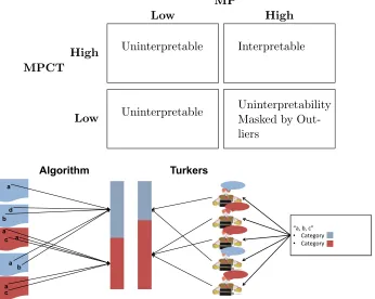
Table 5: Qualitative assessment of the difference between low and high values. When MP is low, a topic is not interpretable regardless of the value of MPCT; when MP is high, a topic is interpretable when MPCT is high, otherwise it has limited interpretability. This is because high MP alone cannot reveal how interpretable a topic is as the topic is differentiable from an outlier term.
MPCT
MP
Low High
High Uninterpretable Interpretable
Low Uninterpretable
Uninterpretability Masked by Out-liers
Algorithm Turkers
a
a
a a
a b
b c
c d
“a, b, c” • Category • Category
Figure 7: An overview of the setup of the topic consensus framework. The left stacked bar comes from the categories of the documents in which tokens appear. The right stacked bar comes from the aggregate of the Turker answers.
5. Topic Consensus
Understanding the underlying distribution of concepts in a topic is important. Since LDA is a mixture model, we can expect some of the topics identified by this model to contain a mixture of different topics. This phenomenon has been documented in the literature as “chimera” topics (Schmidt, 2012). Being able to identify these topics effectively is impor-tant, but we currently do not know how well crowdsourced workers will be able to identify them. In this section we propose a measure, “topic consensus,” which measures how well the mixture of the documents in the LDA topic matches the mixture of labels from the workers.
titles such as “Environment”, and “Judiciary” categories from congressional records (Grim-mer and Stewart, 2013), or “disaster-related” categories from social media (Kireyev et al., 2009). Each title requires a human being to manually read these topics and to assign these category labels. Presumably, good topics should lead to good categories, thus, high topic consensus. Therefore, if there is low topic consensus in terms of categories, topics could be of low interpretability.
5.1 A New Measure for Topic Consensus
We discuss how well the topics from topic modeling conform to the natural categories underlying the text. Explicit topic categories are often present in many corpora, such as newspaper articles, due to their manual categorization by “sections” or categories. For example, our ERC abstracts which explicitly label each abstract with an ERC category, and we measure this conformity to the underlying topic distribution by leveraging the ground-truth topic category labels available as the ERC categories when the abstract is submitted.
The Turkers’ answers reveal the labels that are assigned to topics. By showing the categories to the Turkers as multiple choice questions we can see the category label that a human would assign to the topic. Ideally, we would additionally ask the Turkers to assign confidence scores to their labels to better understand their labeling strategy and to get a better distribution of the category labels. However, since humans are bad at answering questions about themselves (i.e. their own internal confidence) (Bernard and Ryan, 2009), we instead ask many Turkers the same question about the same topic and aggregate the responses. By aggregating the category assignment of Turkers, we can obtain a distribution based on their understanding of the topic.
To understand how well the statistical topics mimic the underlying topics, we show the Turkers the top 20 words of a statistical topic and ask them to choose which of the three categories from that corpus the topic describes. For example, for a given ERC topic, we show the top 20 words along with options for “Life Sciences”, “Physical Sciences”, or “Social Sciences”. We also provide a fourth option, “No Topic Matched”, in case that any of the three categories do not make sense to the Turker. This is depicted in the right half of Figure 7, where Turkers are shown the HIT including top 3 words with 2 categories, and their answers are aggregated to make the distribution of Turker answers. In the figure, instead of 20 top words, top 3 words “a”, “b”, and “c” are chosen to be presented to Turkers. To compute topic consensus, we compare the distribution of the Turkers’ responses for that topic with the distribution of the topic over the ERC categories. To perform this
analysis, we construct an LDA Topic × Category matrix R, where Ri,c indicates topic
i’s probability of occurring in ERC category c. This can be seen in the lefthand side of Figure 7, where the tokens that are labeled with the topic are aggregated based upon the category label of the document they appear in to form the category distribution.
The structure of each row of R is dependent on the type of topic group it comes from.
We construct the row ofR, which correspond to the automated distributions, as follows for
each topic group:
• ERC-* / News-* — The Ri row vector for an ERC topic is created by taking the
for each row (document) ofD labeled with the corresponding ERC category. This is defined as:
Ri,c =
P
j∈McDj,i P
D∗,i
, (5)
whereMcis the set of documents containing the label corresponding to the column of
R, e.g., “SH”, “LS”, or “PE”. This gives us an understanding of the category makeup
for each LDA topic.
• ERCSanitySH-010 / NewsSanityS-010 — The Ri row vector for an SH topic contains a 1 for the sanity category and a 0 for the others. This is due to the way the topics are generated, they contain purely words from that topic.
• ERCRand-010/NewsRand-010— Turkers should not be able to read any defini-tion from a random topic as it consists of random words from the vocabulary. Thus, the row vector for each topic in this set is a 1 for the “N/A” category, and a 0 for the other categories.
Using the responses from the Turkers, we build a separate T opic×Category matrix,
RAMT where RAMTi,j represents the Turkers’ probability of choosing category j when
presented with topic i. In this way, RAMT is the representation of R obtained from the
Turkers’ responses. A row in RAMT indicates the distribution over categories for a given
LDA topic from the Turker’s responses.
The consensus between the responses from the crowdsourced workers and the data is defined as:
consensusmt = 1−J S(R
AMT t||Rt) log2(|c|+ 1)
, (6)
where |c| is the number of categories in the datasets (both the ERC and News datasets
have |c|= 3 categories). We add 1 to account for the presence of the N/A answer. J S is
the Jensen-Shannon divergence (Lin, 1991) between the two distributionsJ S(RAMTt||Rt),
defined as:
J S(RAMTt||Rt) =
K(RAMT
t||M) +K(Rt||M)
2 , (7)
whereK is Kullback-Leibler divergence (Joyce, 2011), and M = 12(RAMTt+Rt).
Jensen-Shannon is a natural choice as the rows ofR andRAMT are probability distributions over
the 3 ERC or News categories and Jensen-Shannon is a measure of the similarity of two
distributions. Jensen Shannon is bounded from [0, log2(|c|+ 1)]; we divide by the upper
bound to yield a number from [0,1]. Finally, Jensen Shannon is a measure of divergence,
meaning that a lower score means that the distributions are more aligned. Thus, we subtract the Jensen Shannon divergence from 1 in order to stay consistent with a consensus measure, where greater consensus means a better topic.
5.2 Topic Consensus Results
Table 6: Confusion matrix of ground truth ERC category assignments of topics against the category assignments made by the Turkers, taken from the outer product of the respective probability distributions. Rows are from the turkers, and columns are from LDA. In the ERC topics, we see that the Turkers are generally able to identify SH and LS topics, but overall fail to identify PE topics. The Turkers perform well when shown random topics, giving most of these topics a “not applicable” label.
ERC-* ERCRand-010 ERCSanitySH-010
Ground Truth
LS SH PE NA LS SH PE NA LS SH PE NA
AMT Classification
LS 29.69 5.21 13.39 0 0 0 0 0.59 0 0.09 0 0
SH 7.96 8.12 10.36 0 0 0 0 3.09 0 9.66 0 0
PE 16.62 8.14 36.21 0 0 0 0 0.61 0 0.11 0 0
NA 16.41 9.38 23.48 0 0 0 0 5.71 0 0.14 0 0
News-* NewsRand-010 NewsSanityS-010
Ground Truth
S B E NA S B E NA S B E NA
AMT Classification
S 35.31 7.74 8.36 0.00 0 0 0 4.26 9.84 0 0 0
B 9.88 50.00 8.61 0.00 0 0 0 1.96 0.04 0 0 0
E 10.00 7.12 21.67 0.00 0 0 0 2.60 0.08 0 0 0
NA 9.10 9.81 7.40 0.00 0 0 0 1.17 0.04 0 0 0
consensus and random topics the lowest consensus, and the performance of the other three topic models are in between.
To further investigate these answers we show a “confusion matrix” that compares the Turkers’ responses with the ground truth in Table 6. Each cell in the matrix is the aggre-gation of the Turker’s responses with the max of all the Turkers taken as the result. This is obtained from the sum of the outer product of the probability distributions from both the turkers (rows), and LDA (columns). The results for ERC-* and News-* topic sets show that most of the topics are understandable. In the case of the “PE” class in the ERC-*
distribution, 52+60+8+252 = 43% of the topics are misclassified as NA. This could be because
0.00 0.25 0.50 0.75 1.00
ERC−010 ERC−025 ERC−050 ERC−100 ERCRand−010
ERCSanitySH−010 Topic Group
T
opic Consensus
TC − ERC
(a) ERC
0.00 0.25 0.50 0.75 1.00
News−010News−025News−050News−100
NewsRand−010NewsSanityS−010 Topic Group
T
opic Consensus
TC − News
(b) News
Figure 8: Topic consensus scores across all models across both corpora. Higher scores are better. On the left we see the form that is shown to the workers. On the right we see that the random topics perform worse than any of the ERC topics, and the SH topics perform the best.
5.3 Using Topic Interpretability Measures
We have employed three measures to identify interpretable topics from topic models thus far: Model Precision, Model Precision Choose Two, and Topic Consensus. At this point we will step back and discuss how to use these measures. There are two clear ways to use these measures. The first is for model selection, and the second is for topic selection.
Model selection is the process of choosing one model out of many (Kohavi et al., 1995). When selecting models for interpretability, we may choose the one that performs best. In
the case of the News data, the model constructed withK = 10 performs best according to
Topic Consensus, and the Model Precision Choose Two measures. Therefore, this model is the best one to choose from the perspective of interpretability.
The other strategy is topic selection. It may be that we are only using topic modeling to describe our dataset, and that we do not need the entire model in order to proceed. In this case, we can use the results of our topic interpretability measures to select a subset of topics that have high interpretability. This is favorable in cases where we need more topics. For example, in the case of Topic Consensus on the ERC data (Figure 8 (a)), we see that
the median of K = 25 outperforms that ofK = 100. However, the top quartile of K = 25
is worse than K = 100. This means that 25 of the 100 topics generated by the K = 100
model are, on average, better than the top 6 topics generated by theK = 25 model. Thus,
decide to use topic selection with a largerK and use the interpretability measures proposed in this work to separate interpretable topics from less-interpretable ones.
6. Automating Measures of Topic Interpretability
In search of measures for topic interpretability, we resort to crowdsourcing approaches to measuring coherence and topic consensus. A natural question is whether we can replace crowdsourcing with automated measures. Crowdsourcing approaches could be costly, or not scalable without funds to recruit a sufficient numbers of Turkers. Furthermore, their results are hard to reproduce without good resources. In short, they present challenges in terms of scalability and reproducibility. The search for automated measures could replace Turkers and make empirical comparison available, saving researchers both time and cost of performing crowdsourced experiments. In this section, therefore, we investigate measures that can be used to automatically measure interpretable topics in terms of coherence and
consensus. Mimno et al. (2011) are among researchers who first try to automate
evalu-ation measures. They generated topics from medical literature and hired physicians, who are subject matter experts in their fields, to rate the quality of topics. They then pro-posed automated measures, Topic Size and Semantic Coherence, to replace these experts for reproducibility. Newman et al. (Newman et al., 2010) proposed a measure based on Pointwise Mutual Information. Aletras and Stevenson (2013) measured the quality of top-ics by inspecting the vector similarity between them. Morstatter et al. (2015) found that the peakedness of the distribution can be used to find interpretable topics. In the following, we introduce these measures, examine their correlations with the three measures of topic interpretability in this work, and then investigate if any of these automated measures can be used to accurately predict measures of topic coherence and topic consensus without the aid of the Turkers.
6.1 Automatic Topic Interpretability Measures
We introduce methods used for automatically assessing the quality of topics. Eight measures are given below:
i. Topic Size (TS):LDA soft assigns documents to topics by hard assigning the tokens within the document to a topic. At the end of training, each token in the corpus will have a topic assigned to it. “Topic Size” is the count of the number of tokens in the input corpus that are assigned to the topic after training. This was used in Mimno et al. (2011) as a possible measure for topic quality. The hypothesis behind this measure is that a larger topic (with more tokens) will represent more of the corpus, and thus will reveal a larger portion of the information within it.
ii. Semantic Coherence (SC):Also introduced by Mimno et al. (2011), this measures the probability of top words co-occuring within documents in the corpus:
SC(w) = |w|
X
j=2
j−1 X
k=1
logD(wj,wk) + 1 D(wk)
where wis a vector of the top words in the topic sorted in descending order, and D is the number of documents containing all of the words provided as arguments. This measure is computed on the top 20 words of the topic.
iii. Semantic Coherence Significance (SCS): We adapt the SC measure above to understand the significance of the top words in the topic when compared to a random set of words. To calculate this measure we select 100 groups of words at random, following the topic’s word distribution. We then recompute the Semantic Coherence
measure for each of the random topics, obtaining a vector,d, of topic coherence scores.
We calculate the mean, ¯d, and standard deviation,std(d). Significance is defined as:
SCS(w) = SC(w)−d¯
std(d) . (9)
iv. Normalized Pointwise Mutual Information (NPMI): Introduced by Bouma (2009), this metric measures the probability that two random variables coincide. This measure was used to estimate the performance of Model Precision in Lau et al. (2014),
where the authors adapted it to measure the coincidence of the top |w| words. In
this paper, two variables “coinciding” is the probability that they will co-occur in a document. The authors named this version OC-Auto-NPMI, formally:
OC-Auto-NPMI(w) =
|w|
X
j=2
j−1 X
k=1
log PD(wj,wk)
PD(wj)PD(wk) −log(PD(wj,wk))
, (10)
where PD(·) = D(·)/|N|, where |N| is the number of documents in the corpus. PD
measures the probability that a document in the corpus contains the words given to
D(·). Going forward, we will refer to this measure as NPMI.
v. Category-Distribution HHI (Cat-HHI):The Herfindahl-Hirschman Index (Hirschman, 1945), or HHI, is a measure proposed to find the amount of competition in a market. This is calculated by measuring the market share of each firm in the market, formally:
HHI = (H−1/N)
(1−1/N), (11)
WhereH=P
is2i,N is the number of firms in the market, andsi is the market share
of firmi, as a percentage. HHI ranges from 0 to 1, with 1 being a perfect monopoly
(no competition), and 0 being an evenly split market. In this way we measure how focused the market is on a particular firm.
By treating the corpus categories as firms, and the market share distribution as Ri,
we can calculate how focused each topic is around a particular category.
vi. Topic-Probability HHI (TP-HHI): Using the same formulation as ERC-HHI,
this time we treat every word in the vocabulary as a firm, and Tmi as the probability
purely on the peakedness of the distribution. This measures whether the focus of a topic is around a handful of words, or whether it is evenly spread across the entire vocabulary used to train the model.
vii. No. of Word Senses: The total number of word senses, according to WordNet, of the top five words in the topic. This varies slightly from the measure proposed in (Chang et al., 2009), where the authors also consider the intruded word. Because the intruded word is generally far away, we exclude it from our calculation.
viii. Avg. Pairwise JCD:The Jiang-Conrath (Jiang and Conrath, 1997) distance (JCD)
is a measure of semantic similarity, or coherence, that considers the lowest common
subsumer according to WordNet. Here we compute the average JCD of all 52
= 10 pairs of the top five words of the topic. This approach was introduced by (Chang et al., 2009), however we modify it slightly to only consider the topic’s top five words.
ix. Lesk Similarity: The Lesk Algorithm (Banerjee and Pedersen, 2002) for word sense disambiguation uses WordNet to identify the most appropriate synset for an ambigu-ous word given a context. Following the use of this algorithm in (Newman et al., 2010), we adopt this technique in our automated measures. To turn the synset re-turned by this algorithm into a similarity measure, we evaluate the path similarity from the synset returned by this algorithm and all of the synsets in the context. The “context” is defined as the top 5 words in the topic, and the “ambiguous word” is the intruded word. When applying this to consensus, we use the same intruded word as in the MP and MPCT case.
6.2 Correlation with Crowdsourced Measures of Topic Interpretability
To see how well these automatic topic measures compare with the crowdsourced topic
mea-sures from the “Topic Interpretability” section, we calculate the Spearman’s ρ (Spearman,
1904) rank correlation coefficient between the crowdsourced measure and the automatic measure. The correlations between each pair of crowdsourced and automatic measure are
shown in Table 7. In this table, we present the Spearman’s ρ, as well as an indication of
the significance level for the following hypothesis test:
H0 : The two sets of data are uncorrelated.
Instances where the hypothesis is rejected at theα= 0.05 significance level are shown in
Ta-ble 7. We see that the measure most correlated with Model Precision and Model Precision Choose Two (MPCT) is Avg. Pairwise JCD, meaning that documents whose words have a higher semantic similarity are more likely to achieve higher Model Precision (MP) values. We see that higher (better) values of Model Precision are accompanied by higher average JCD values. Table 7 shows the measure most correlated with Topic Consensus (TC) is TP-HHI. These correlations lead us to the next question: can we predict each of the three measures (MP, MPCT, and TC) of topic interpretability based on their correlations?
6.3 Predicting Crowdsourced Values of Topic Interpretability Measures
While correlation can be used to find the quality of a measure, we further ask if it is feasible
Table 7: Spearman’sρ between measures requiring Mechanical Turk and automated
mea-sures. Instances where we reject the null hypothesis at the significance level ofα= 0.05 are
denoted with ∗, and instances where we reject the null hypothesis at the significance level
of α= 10−4 are denoted with∗∗.
ERC-* News-*
MP MPCT TC MP MPCT TC
TS 0.152∗ -0.709∗∗ 0.532∗∗ -0.585∗∗ -0.645∗∗ 0.688∗∗
SC 0.359∗∗ -0.165∗ 0.584∗∗ -0.443∗∗ -0.885∗∗ 0.163∗
SCS -0.074 -0.582∗∗ 0.788∗∗ -0.337∗∗ -0.410∗∗ 0.501∗∗
NPMI -0.562∗∗ 0.067 0.774∗∗ 0.189∗ -0.203∗ 0.674∗∗
Cat-HHI 0.103 -0.652∗∗ 0.478∗∗ -0.223∗ -0.416 0.588
TP-HHI -0.471∗∗ -0.057 0.885∗∗ -0.001 -0.318∗ 0.913∗∗ Senses -0.111 -0.267∗ 0.854∗∗ -0.055 0.022 0.674∗∗
JCD 1.000∗∗ 0.750∗∗ 0.022 0.685∗∗ 0.805∗∗ 0.349∗∗
Lesk 0.050 -0.034 0.189∗ 0.533∗∗ 0.503∗∗ 0.442∗∗
Table 8: Errors of the predictive algorithm trained on all of the automated measures.
Results are presented as RMSE ± the standard deviation. These results indicate that
Topic Consensus is the most predictable.
Model Precision Model Precision Choose Two Topic Consensus
ERC-* 0.280±0.039 0.352±0.064 0.131±0.021
News-* 0.239±0.049 0.307±0.075 0.114±0.034
the most correlated measure may be the most predictive, however, due to nonlinear patterns within the data this may not be the case. In this section, we investigate if we can predict the true scores of topic interpretability by using the above eight automated measures.
7. Conclusion and Future Work
Statistical topic models are a key component for machine learning, NLP, and the social sciences. In this work we investigate different measures for the interpretability of the topics
generated by these approaches. We view topic interpretability from two perspectives: topic
coherence and topic consensus. Coherence measures how semantically close the top words of a topic are. Consensus measures the agreement between the mixture of labels assigned by the humans and the mixture of labels from the documents assigned to the topic. We investigate what is needed for comprehensive measure of each perspective, understand how different these measures for topic coherence and consensus are, and show their experimental results using real-world datasets.
For topic coherence, we study Model Precision (MP) and propose Model Precision Choose Two (MPCT). The two measures complement each other to better measure the semantic closeness of topic words. MP works by making sure that the topic words should be far away from the intruded word. Additionally, MPCT complements MP by addressing the closeness of the 5 words within the topic. We compare MPCT with MP and show how these two measures can work in tandem to identify interpretable topics. One natural question that can arise from the MPCT setup is why only two words are requested, when in fact any number of words could be asked for. While this is theoretically attractive, the practical implications for the Turkers can present a challenge. By asking them to select one intruder and one additional word, we present a small, viable workload for the Turkers. Finding more strategies to effectively measure coherence is an area for future work.
For topic consensus, we assess how well the workers’ aggregate understanding of the topic matches the aggregate of the categories provided by the corpus. In both corpora, each document is tagged with a category. When we train a topic model, each topic will ultimately be a mixture of these categories. This method reveals how well the topics generated can be understood in relation to the underlying categories in the corpus. One natural application
of this measure is to identify chimera topics, i.e. those topics that are split between two
concepts or categories. Furthermore, by inspecting the Turker’s results on known topics, we can see the bounds of this measure on extremely good, and extremely bad topics.
All three measures of topic interpretability rely on crowdsourcing platforms, which mo-tivates a need to automate them in order to improve reproducibility and scalability. Recre-ating these results with human workers requires significant investments of time to recruit the workers, as well as funds to pay them. We investigate how to estimate these crowd-sourced topic measures without the need of crowdsourcing tools such as Mechanical Turk. We find some automated measures that are highly correlated with crowdsourced measures (MP, MPCT, and TC), allowing researchers to reproduce these topic quality measures at scale. In addition, we propose to construct a prediction model for predicting MP, MPCT, and TC based on the automated measures. This prediction model can take advantage of new automated measures to improve their predictive power.