Learning Behavior-Selection by Emotions and Cognition in a Multi-Goal Robot Task

Learning Behavior-Selection by Emotions and Cognition in a

Multi-Goal Robot Task

Sandra Clara Gadanho [email protected]

Institute of Systems and Robotics IST, 1049-001 Lisbon, Portugal

Editor: Peter Dayan

Abstract

The existence of emotion and cognition as two interacting systems, both with important roles in decision-making, has been recently advocated by neurophysiological research (LeDoux, 1998, Damasio, 1994). Following that idea, this paper presents theALECagent architecture which has both emotive and cognitive learning, as well as emotive and cognitive decision-making capabili-ties to adapt to real-world environments. These two learning mechanisms embody very different properties which can be related to those of natural emotion and cognition systems.

The reported experiments test ALECwithin a simulated autonomous robot which learns to perform a multi-goal and multi-step survival task when faced with real world conditions, namely continuous time and space, noisy sensors and unreliable actuators. Experimental results show that both systems contribute positively to the learning performance of the agent.

Keywords: Emotion, hybrid learning, autonomous robots

1. Introduction

The purpose of the work reported here is to build an autonomous robot controller which can learn to master a complex task when situated in a realistic environment (i.e., an environment endowed with real-world problems such as continuous time and space, noisy sensors and unreliable actuators). The robot’s task has several features that pose serious difficulties to the learning algorithm:

• it has multiple goals which may conflict with each other;

• there are situations in which the agent needs to temporarily overlook one goal in order to accomplish another successfully;

• the agent has short-term and long-term goals;

• a sequence of different behaviors may be required to accomplish a certain goal;

• the behaviors are unreliable: they may fail or they may lead the agent to undesirable situations; • the behaviors’ appropriate duration is undetermined, it depends on the environment and on

their success.

To solve this problem, Gadanho and Hallam (2001b) propose an emotion-based architecture (EB architecture) in which a traditional reinforcement learning adaptive system is complemented with an emotion system responsible for both reinforcement and behavior switching. The agent has some innate emotions that define its goals, and it then learns emotion associations of environment-state and behavior pairs, which determine its decisions. The agent uses a Q-learning algorithm to learn its behavior-selection policy while it interacts with its environment. The policy is stored in neural networks, which limits memory usage substantially and accelerates the learning process, but can also introduce inaccuracies and does not guarantee learning convergence (Sutton and Barto, 1998).

The ALEC (Asynchronous Learning by Emotion and Cognition) architecture proposed here

aims at a better learning performance by augmenting the EB architecture with a cognitive system which complements its current emotion-based adaptation capabilities with explicit rule knowledge extracted from the agent-environment interaction. The different learning capabilities of the two systems and their interaction have the potential to produce a more powerful adaptive system. The cognitive system is based on the adaptive rule-decision system proposed within theCLARIONmodel (Sun and Peterson, 1998) which allows learning the decision rules from the agent-environment interaction in a bottom-up fashion.

In summary, a modified version of theEBarchitecture, theEBIIarchitecture, is considered to be the emotion system ofALECand the added rule system is considered to be its cognitive system. The distinctive underlying learning mechanisms of the two systems are consistent with the assumption that, in nature, the cognitive system can make more accurate predictions based on rules while the emotional associations have less explanatory power but can make more extensive predictions and predict further ahead in the future.

In the next section, there is a short review of related work. This is followed by a detailed description of the EBIIarchitecture and of the full ALEC architecture. In the experiments section, both the EBII and the ALEC architectures are tested and compared with alternative architectures (including the EBarchitecture) in a robot task with the features mentioned above. Three different versions ofALEC were tested, two testing alternative cognitive systems and a third one testing a simplified emotion system. While the first cognitive system was directly inspired by the top-level of theCLARIONmodel, the second version takes advantage of the new underlying architecture. The third version of ALEC follows earlier experiments which suggested that the emotion system may be exclusively dedicated to learning about goal state and that learning about goal state transitions could be left to the cognitive system alone. An non-asynchronous controller namedLEC (Learning by Emotion and Cognition) was also tested to demonstrate the usefulness of the behavior-switching mechanism ofALEC. Finally, theALECarchitecture is discussed and conclusions are drawn.

2. Background

Learning low-level behaviors consists of deciding between simple reactive actions on a step-by-step basis. However, in learning behavior selection, apart from deciding which behavior to select, the controller must also decide when to switch and reinforce behaviors. There are various reasons why a behavior may need to be interrupted: it has reached its goal; it has become inappropriate due to changes in the environment situation; or it is not able to succeed in its goal. In practice, the duration of behaviors must last long enough to allow them to manifest themselves and short enough so that they do not become inappropriate (due to changing circumstances) long before being interrupted. The correct timing of behavior-switching can be vital (Gadanho and Hallam, 2001a).

The problem of deciding when to change behavior is not an issue in traditional reinforcement learning problems, because these usually consist of grid worlds in which a single discrete action moves the agent to one of the cells in the neighborhood of the cell where the agent is located. Once the cell transition occurs, the agent is in a new state (each cell is a state) where it is clearly appropriate to take a new learning step, i.e. evaluate the previous action and make a new selec-tion. In a continuous world, the determination of a state transition is not clear. In robotics, agent states change asynchronously in response to internal and external events, and actions take variable amounts of time to execute (Mataric, 1994). As a solution to this problem, some researchers extend the duration of the current action according to domain-dependent conditions of goal achievement or action applicability (e.g., Mahadevan and Connell, 1992, Lin, 1993, Mataric, 1994). Others interrupt the action when there is a change in the perception (e.g., Rodriguez and Muller, 1995, Asada, 1996). However, this may not be a very straightforward solution when the robot is equipped with multiple continuous sensors that are vulnerable to noise. Marom and Hayes (2000) go a step further by auto-regulating the degree of discrimination of new events in an attempt to maintain a constant attentional effort.

Inspired by literature on emotions, empirical work with the EB architecture (Gadanho and Hallam, 2001b,a) has shown that reinforcement and behavior-switching can easily be addressed together by an emotional system. The justification for the use of emotions is that, in nature, emotions are usually associated with either pleasant or unpleasant feelings that can act as reinforcement (e.g., Tomkins, 1984, Albus, 1990, Bozinovski, 1982) and are frequently pointed to as a source of interruption of behavior (Sloman and Croucher, 1981, Simon, 1967).

Extensive empirical results presented by Gadanho (1999) have demonstrated that the EB archi-tecture is quite competent, and results presented in this paper demonstrate thatEBIIhas similar per-formance. However, it was felt that the learning abilities of these architectures could be improved. The adaptation mechanisms shared by these architectures can only provide implicit knowledge, which limits the range of decision capabilities available to the agent at any one point. The agent learns the relative utility of each behavior and can make a decision based on that, but it has no knowledge on how this information was collected. This prevents the use of more advanced planning techniques which rely on explicit knowledge of cause and effect (e.g., if agent is in situation S and selects action A, then X happens). Furthermore, in special cases, the generalization abilities of the neural-networks can sometimes work against the agent by preventing the acquisition of very fine-tuned information in information-rich portions of the state space. In fact, strong opposite outcomes in neighboring states can easily be merged and recorded as neutral outcomes.

To address these limitations, theALECarchitecture adds a cognitive system to theEBII architec-ture. The function of the cognitive system is to provide an alternative decision-making process to the emotion system, relying on a collection of important discrete rule-based cases built by the agent. This alternative memory representation has two main advantages: it is not prone to the inaccuracies due to neural-network over-generalization and it may allow the use of more conventional A.I. techniques such as planning.

The cognitive system collects knowledge independently and should step in to correct the emo-tion system’s decisions. The cognitive system used here is based on the rule-based level of the CLARION model (Sun and Peterson, 1998, Sun et al., 2001). The CLARION model is a hybrid cognitive model which has two decision-making levels, each with different learning capabilities. The bottom-level is a Q-learning system that uses neural-networks and is similar to a subsystem of the emotion system of ALEC (more specifically, the adaptive system presented in Section 3.2). In particular, it shares with ALEC’s emotion system the same problems of inaccuracies due to the blurring effect of the neural-networks generalization abilities. The top-level is a rule-based system that collects knowledge independently and complements the bottom-level by detecting and correct-ing over-generalization (Sun and Peterson, 1998). However, the top-level learncorrect-ing capabilities are limited and dependent upon the bottom-level, since the top-level has no form of temporal credit assignment and needs the bottom-level’s long-term predictions. The main reason for selecting CLARION’s rule system is that it is not derived from a pre-constructed set of rules given externally. Instead, rules are extracted from the agent-environment interaction experience through the medi-ation of low-level skills. Other rule models are usually top-down, i.e. through practice the agents transform high-level knowledge into usable procedural skills (Sun et al., 2001). Nevertheless, a

priori knowledge can still be given easily to the system in the form of rules and if these are useful

they will be assimilated into procedural knowledge by the system (Sun et al., 2001).

perceptual path performs the “quick and dirty” processing usually associated with emotions. The cognitive path attempts to provide a more sophisticated evaluation using higher-level reasoning. These layers may have their own separate learning mechanisms for adapting their evaluations, but in the experiments the perceptual evaluation is usually implemented as innate fixed knowledge and the cognitive layer always learns from scratch. In the DARE model, the perceptual layer extracts relevant features and the cognitive layer’s task is to identify objects. Nevertheless, a feature of its implementations which it shares with ALEC is that the perceptual layer has a non-differentiated evaluation of events according to their main characteristics, while the cognitive layer accumulates a set of individual instances of events. The DARE model differs fromALECin the kind of learning mechanisms used (in general consisting of stimulus matching using Euclidean distances, at two levels of complexity) and the type of problems it addresses (the learning abilities are generally applied to stimulus evaluation and the problems derived from the interaction of the agent with a real world are often ignored).

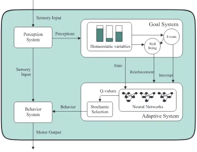
3. EBIIArchitecture

Figure 1: TheEBIIarchitecture.

specifically, it calculates a well-being value that is used as reinforcement by the adaptive system and determines the trigger steps, i.e. the steps when relevant events are detected. The adaptive system learns which behavior to select at trigger steps, using reinforcement-learning techniques that rely on neural-networks to store the utility values. The two systems are described in detail next.

3.1 Goal System

The goal system’s role is to complement a traditional reinforcement-learning adaptive system so that the learning is autonomous, i.e. independent of external influences. The goal system determines how well the adaptive system is doing, or more specifically, determines the reinforcement due at each step. Moreover, the goal system is responsible for deciding when behavior switching should occur. The EB architecture addressed the problem of the goal system by using an emotional model. A mixture of perceptual values and internal values were used in the calculation of a single multi-dimensional emotional state. This state, in turn, was used to determine the reinforcement at each time step and significant differences in its value were considered to be relevant events used to trigger the behavior selection mechanism.

The EBIIarchitecture presented here has been modified to emphasize the multiple goal nature of the problem at hand and identify and isolate the different aspects of the agent-environment interaction that need to be taken into consideration when assessing the agent overall goal state.

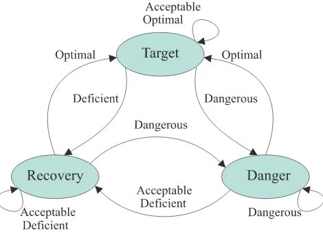
The goals are explicitly identified and associated with homeostatic variables. These homeostatic variables are associated with three different states: target, recovery and danger. The state of each variable depends on its continuous value, which is grouped into four qualitative categories: optimal, acceptable, deficient and dangerous. The variable remains in its target state as long as its values are optimal or acceptable, but it only returns to its target state once its values are optimal again. This state transition is akin to that of a thermostat in that a greater deviation from the target values is required to change from a target state into a recovery state than the inverse transition. The danger state is directly associated with dangerous values and implies that recovery is urgent. Details of state transitions are shown in Figure 2, and an example of the categorization of the continuous values of a homeostatic variable is shown in Figure 3.

Figure 3: An example of a categorization of the continuous values of a homeostatic variable.

To reflect the current hedonic state of the agent, a well-being value is derived from the above. This value depends primarily on the state values of the homeostatic variables. If a variable is in the target state it has a positive influence on the well-being, otherwise it has a negative influence which is proportional to its deviation from target values.

The well-being is also influenced by the following events:

State change — when a homeostatic variable changes from one state to another the well-being is

influenced positively if the change is towards a better state and negatively otherwise;

Prediction of state change — when some perceptual cue predicts the state change of a

homeo-static variable, the influence is similar to the above, but lower in value, and dependent on the accuracy of the prediction and on how soon the state change is expected. In particular, if a transition to the target state involves a sequence of steps then a positive prediction is made any time a step is accomplished. The intensity of the prediction increases as the number of steps to finish the sequence is reduced. Predictions are always associated with individual homeostatic variables and are only made if the corresponding variable value is not optimal.

These two events were modeled after emotions, in the sense that they result from the detection of significant changes in the agent’s internal state or predictions of such changes. In the same way that emotions are associated with feelings of “pleasure” or “suffering” depending on whether a change is for the better or not, these events influence the well-being value such that the information of how good the event is is conveyed to the agent through the reinforcement. One may distinguish between the emotion of happiness when a target is achieved (or predicted to be achieved) and the emotion of sadness when a target state is lost (or about to be lost).

The primary influence of the homeostatic variables, on the other hand, is modeled after the natural background emotions which reflect the overall state of the agent in terms of maintaining homeostasis (Damasio, 1999).

φ = csrs+

∑

ct(sh)wh+cp

∑

h∈H

rphwh (1)

Coefficient Definition Value

cs State coefficient 0.6

ct(sh) State-transition coefficient

state of h did not change 0.0

state of h changed from to

– target 1.0

– danger -1.0

target recover -0.4

danger recover 0.4

cp Prediction coefficient 0.2

Table 1: Coefficient values used in the calculation of the well-being value. These values were selected to reflect the relative importance of the different influences.

between 0 and 1.

rs =

(

1 if

_H

−max h∈H−(d

n_(v

h)wh) otherwise (2)

dn(vh) = d(vh)/dhmax (3)

H

H

The influence of state on well-being is expressed by rs described in Equations 2, 3 and 4. This value is 1 if the homeostatic variables are all in their target values or improving their values (i.e. d(vh)is decreasing). Otherwise, it depends on the normalized deviation from optimal values (dn(vh), defined in Equation 3), i.e. the distance (d(vh)) of the current value (vh) of the homeostatic variable (h) to the nearest optimal value normalized by the maximum possible distance (d_hmax, see example in Figure 3) of any value of this homeostatic variable to a optimal value. This ensures that

dn(vh)is always between 0 and 1.

The values of predictions rp_h depend on the strengths of the current predictions and vary between -1 (for predictions of no desirable changes in the homeostatic variable h) and 1 (for predictions of desirable changes). If there is no prediction then rp_h=0. The values of rp_h are domain-dependent.

The goal events, i.e. state change and prediction of state change, are also responsible for trig-gering the adaptive system for a new behavior selection. The adaptive system only performs a reinforcement-learning step, i.e. evaluates the current behavior and makes a new behavior-selection, during trigger steps. On other steps, the previous selected behavior is kept and there is no policy update. The adaptive system is triggered when an event (one of the two described above) is detected.

3.2 Adaptive System

Traditional Q-learning usually employs a table which stores the utility value of each possible action for every possible world state. In a real environment, the use of this table requires some form of partition of the continuous values provided by sensors. An alternative to this method suggested by Lin (1993) is to use neural networks to learn by back-propagation the utility values of each action. This method has the advantage of profiting from generalization over the input space and being more resistant to noise, but on the other hand the on-line training of neural-networks may not be very accurate. The reason being that the neural networks have a tendency to be overwhelmed by the large quantity of consecutive similar training data and forget the rare relevant experiences. Using an asynchronous triggering mechanism, such as the one proposed by the current architecture, can help with this problem by detecting and using only a few relevant examples for training.

The state information fed to the neural-networks comprises the homeostatic variable values and other perceptual values gathered from the robot sensors.

The developed controller tries to maximize the reinforcement received by selecting between one of the available hand-designed behaviors.

At each trigger step, the agent may select between performing the behavior that has proven to be better in the past and therefore has the best utility value so far, or selecting an arbitrary behavior to improve its information about the utility of that behavior. The selection function used is based on the Boltzmann-Gibbs distribution and consists of selecting a behavior with higher probability, the higher its utility value in the current state.

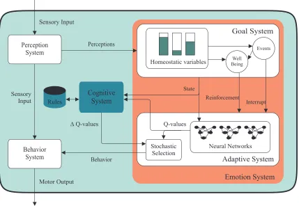
4. ALECArchitecture

TheALEC architecture — see Figure 4 — is an extension of theEBIIarchitecture described previ-ously. It basically has an additional cognitive system based on the rule system ofCLARION. The two major systems of the ALECarchitecture, the emotion and the cognitive systems, are described next.

4.1 Emotion System

The emotion system ofALEC is composed by the goal system and the adaptive system of theEBII architecture described previously.

Apart from having learning mechanisms with capabilities analogous to those of natural emo-tions, the emotion system is composed of two systems that can be related to emotions.

The goal system itself was originally an emotion model because its functions, i.e. reinforcement and behavior interruption, are usually associated with emotions in natural systems. In the EBII version, this emotion model has been replaced, but its mechanisms are still strongly inspired by emotions. This system produces a well-being value which is derived from the agent’s internal state, i.e. its homeostatic variables, by emotion-like processes. In this case, and as defended by Damasio (1999), emotion processes are intrinsically related to the maintenance of the homeostasis of the individual. One could argue that the well-being value is an emotional feeling that provides a summary of the overall state of the agent.

Figure 4: TheALECarchitecture.

the options available to the agent, in terms of the agent’s internal goals and based on previous experiences.

4.2 Cognitive System

Two different versions of the cognitive system were tested separately in the experiments. The first is directly inspired by the rule system of the CLARION model and the second version has a few innovations.

4.2.1 VERSIONI

The cognitive system maintains a dynamic collection of rules which allows it to make decisions based on past positive experiences. Each individual rule consists of a condition for activation and a behavior suggestion. The activation condition is dictated by a set of intervals, one for each dimension of the input space. The granularity of the possible interval ranges is determined a priori, thus a condition interval may only start or end at pre-defined points of the input space. This may represent a very large number of possible states.1 For this reason, rule learning is limited to those 1. In the experiments, there are 6 input dimensions varying between 0 and 1 and it was decided to segment each input

few cases for which there is a particularly successful behavior selection, leaving the other cases to the emotion system which makes use of its generalization abilities to cover all the state space.

If a behavior is found to be successful in a particular state then the agent extracts a rule corre-sponding to the decision made and adds it to its rule set. Subsequently, whenever the same decision is made again the agent updates the record of the success rate of the rule (SR). This is recorded in terms of time-weighted statistics of the number of times the decision resulted in success (PM) and the number of times it did not (NM). These statistics are incremented by one in the appropriate trigger steps and are decreased by 0.001 of their value in every trigger step.

The success of the agent is measured in terms of its immediate reinforcement r and of the difference of Q-values between the state x where the decision a was made and the state y reached after the decision was taken (as in Equation 5, whereγis the reinforcement-learning discount factor and Tsuccess is a constant threshold). This means that rule learning takes into consideration the information collected by the emotion-system.

r+γmaxbQ(y,b)−Q(x,a)>Tsuccess (5)

If the rule is often successful, the agent tries to generalize it by making it cover a nearby environmental state. If the rule’s success rate is very poor then the agent attempts to make it more specific. If this does not improve the success rate, or the rule only covers one state, then the agent deletes the rule. Statistics are kept for the success rate of every possible one-state expansion or shrinkage of the rule, so that the best option may be selected. The exact conditions for expansion and shrinkage of a rule are defined by Equations 6 and 7, respectively. The rule is compared against a match-all rule with the same behavior suggestion (ruleall) and against itself after the best expansion or shrinkage (ruleexpand and ruleshrink, respectively). A rule is expanded if it is significantly better than the match-all rule and the expanded rule is better or equal to the original rule. A rule that is insufficiently better than the match-all rule is shrunk if this results in an improvement or otherwise is deleted. The comparison is made in terms of the information gain (IG) of the success rate as defined in Equations 8 and 9. The information gain measures the improvement of the success rate of rule1 relative to rule2. The success rate is calculated based on the time-weighted statistics gathered for each rule and converges to 0.5 if the rule condition is not met again. The thresholds T_expand and

T_shrinkare positive constants which obey the condition T_expand>T_shrink.

IG(rule,ruleall)>Texpand ∧ IG(ruleexpand,rule)≥0 (6) IG(rule,rule_all)<T_shrink ∧ IG(rule_shrink,rule)>0 (7)

IG(rule1,rule2) = log2(SR(rule1))−log2(SR(rule2)) (8)

SR(rule) = PM(rule) +1

PM(rule) +NM(rule) +2 (9)

Apart from being deleted due to bad performance, rules are also deleted if their condition has not been met for a long time. In particular, when the maximum number of rules has been reached, the creation of a new rule requires the elimination of the rule that has not been used for the longest time.

Success statistics are reset whenever the rule is modified by a merging, expansion or shrinkage. If the cognitive system has a rule that applies to the current environmental state, then the cognitive system influences the behavior decision. It makes the selection of the behaviors suggested by the rules more probable by adding an arbitrary constant value of 1.0 to the respective Q-value before the stochastic behavior selection is made.

This first version of the cognitive system is based on the rule system of CLARION (Sun and Peterson, 1998) with no addition. The format of the rule’s activation condition inALECconsists of a single continuous interval of values instead of a set of intervals for each dimension of the input space. This new format is computationally advantageous, albeit less flexible. Furthermore, the rule system of CLARION has two different, but very similar, success criteria: one for extraction (the decision whether a rule should be created) and another for rule modification (the update of PM and NM). However, preliminary experiments carried out in the course of the current work showed that having different criteria or having just one applied to both cases did not affect the performance of the system.2 Another simplification made was the elimination of the lists of child rules associated with each rule. These allow each rule to maintain a record of previously existent rules which had been subsumed by the rule, so that once a rule was deleted the child rules could be recovered. The extra complexity introduced by this list mechanism was not considered worthwhile.

4.2.2 VERSIONII

The second version of the cognitive system attempts to take advantage of the properties of the ALEC architecture. More specifically, it has a new success criterion which relies on the goal system’s homeostatic-variable transitions. Instead of using Equation 5 to determine if a behavior is successful, it considers that a behavior is successful if there is a positive homeostatic variable transition, i.e. if there is a state transition event that consists of an improvement of a variable state — more specifically, if a variable state changes to the target state or from the danger state.

5. Experiments

This section describes the experiments in detail. It starts with a description of the task and the domain-specific implementation details of the controllers. This is followed by an explanation of the experimental procedure and the presentation of the results.

5.1 Robot Task

The aim of ALEC is to allow an agent faced with realistic world conditions to adapt on-line and autonomously to its environment. In particular, the agent should be able to cope with continuous time and space while constrained by limited memory, time constraints, noisy sensors and unreli-able actuators. Furthermore, the agent is required to perform a task with multiple and sometimes conflicting goals, which may require sequences of actions to be completed.

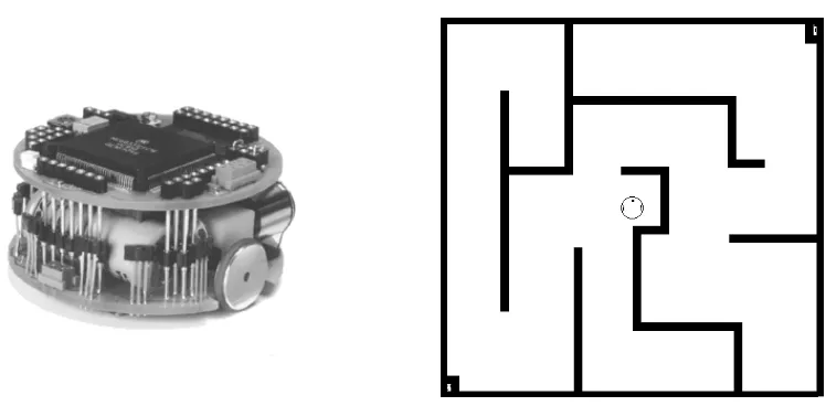
Experiments were carried out in a realistic simulator (developed by Michel, 1996) of a Khepera robot — a small robot with left and right wheel motors, and eight infrared sensors that allow it to detect object proximity and ambient light. Six of the sensors are located in the front of the robot and two in the rear. The experiments evaluate the agent in a survival task that consists of maintaining adequate energy levels in a closed maze-like environment — Figure 5 — with some walls and two

Figure 5: The Khepera robot and its simulated environment.

lights surrounded by bricks on opposite corners. The robot can acquire energy from energy sources which are associated with the lights so that the robot can sense them when nearby. The robot wastes a small amount of energy in every step, which increases with its usage of the motors.

The extraction of energy is complicated by requiring the agent to learn sequences of behaviors and temporarily overlooking the goal of avoiding obstacles in the process. To gain energy from an energy source, the robot has to bump into it. This will make energy available for a short period of time. It is important that the agent is able to discriminate the existence of available energy, because the agent can only get energy during this period. Energy is obtained by receiving high values of light in its rear light sensors, which means that the robot must quickly turn its back to the energy source as soon as it senses that energy is available. To receive further energy, the robot has to restart the whole process by hitting the light again so that a new time window of released energy is started. The goal of maintaining energy also requires the robot to find different energy sources in order to survive. An energy source can only release energy a few times before it is exhausted. In time, the energy source will recover its ability to provide energy again, but meanwhile the robot is forced to look for other sources of energy in order to survive. The robot cannot be successful by relying on a single energy source, i.e. the time it takes for new energy to be available in a single energy source is longer than the time it takes for the robot to waste that energy. When an energy source has no energy, the light associated with it is turned off and it becomes a simple obstacle for the robot.

In summary, the agent has three goals: to maintain its energy, avoid collisions and move around in its environment.

5.2 Controllers’ Setup

The state information that is fed to the neural-networks and the rule’s state conditions are the homeostatic variable values and three perceptual values: light intensity, obstacle density and energy availability. The energy availability value indicates whether a nearby energy source is releasing energy.

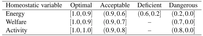
Homeostatic variable Optimal Acceptable Deficient Dangerous Energy [1.0,0.9] (0.9,0.6] (0.6,0.2] (0.2,0.0]

Welfare [1.0,0.9] (0.9,0.7] – (0.7,0.0]

Activity [1.0,1.0] (0.9,0.8] – (0.8,0.0]

Table 2: Value intervals of the different qualitative categories of the homeostatic variables.

conditions, fail to attain their goal. On the other hand, the wall-following behavior may lead the robot to crash, i.e. become immobilized against a wall. It is part of the robot’s task to be able to cope with these limitations.

Three homeostatic variables were identified:

Energy — is the battery energy level of the agent and reflects the goal of maintaining its energy;

Welfare — maintains the goal of avoiding collisions, this variable is in its target state when the

agent is not in a collision situation;

Activity — ensures that the agent keeps moving, if the robot keeps still this value slowly decreases

until eventually its target state is not maintained.

These variables are directly associated with the robot goals mentioned previously. Their associ-ated weights (wh) are 1.0 for energy, 0.6 for welfare and 0.4 for activity. These weights reflect the relative importance of the goals. The most important tasks are for the agent to maintain its energy and avoid obstacles when possible — the activity goal is secondary. The homeostatic-variable values were categorized according to Table 2 based on observations of the variable values and a subjective qualitative appreciation of the correspondent situation of the agent. The selection of the categories values did not require any tuning and the system was quite robust to slight variations on the weight values.

State change predictions were only considered for the energy and the activity variables (r_pwelfare= 0). In the energy case, two predictions are made. A small value prediction is made whenever the light detected by the sensors is above a threshold and its value has just changed significantly.3 Another, higher-valued, prediction is made whenever the agent detects significant changes in energy available to re-charge. The actual values of the predictions are:

• r_penergy = p(Ia) with function p as defined in Equation 10 and with Ia being the energy availability, when the agent detects significant changes in energy availability; or

• r_penergy=p(Il)/2 with Ilequal to light intensity, if there is solely a detection of a light change and Il>0.4.

p(I) =

I I value has increased

−0.5(1−I) I value has decreased (10)

The activity prediction provides a no-progress indicator given at regular time intervals when the activity of the robot is low for long periods of time. This is, in fact, a negative prediction (r_pactivity=−1), because it predicts future failure in restoring activity to its target state (should the current behavior be maintained) since the behavior has failed to do so within a reasonable amount of time. It is important that the agent’s behavior selection is triggered in these situations, otherwise a non-moving agent will eventually run out of events.

The rule system’s thresholds are set to Tsuccess =0.2, Tshrink =1.0 and Texpand =2.0. The maximum number of rules is 100. The six input dimensions of the rule conditions were segmented with 0.2 granularity, meaning that condition intervals can start or end at 0, 0.2, 0.4, 0.6, 0.8 and 1. An example of a possible rule is: if energy ∈[0.6,1]and activity∈[0,1]and welfare∈[0,0.6]and light intensity ∈[0,1]and obstacle density∈[0.8,1]and energy availability ∈[0,1]then execute behavior avoid obstacles. Note that the parts of the condition requiring values to be in the interval [0,1]are always true and could be omitted.

Unless otherwise specified the tested architectures share the features and setup of the EB archi-tecture which is described in detail in Gadanho and Hallam (2001b), apart from a minor increase in difficulty level (lower energy autonomy than previously).

5.3 Procedure

An experiment was performed for each controller tested. Each experiment consisted of one hundred different robot trials of three million simulation steps. In each trial, a new, fully recharged, robot with all state values reset was placed at a randomly selected starting position. For evaluation purposes, the trial period was divided into sixty smaller periods of fifty thousand steps. For each of these periods the following indicators were recorded:

Reinforcement — mean of the reinforcement (or well-being) value calculated at each step;

Energy — mean energy level of the robot;

Distance — mean value of the Euclidean distance d, taken at one-hundred-step intervals,4_between the opposing points of the rectangular extent containing all the points the robot visited during the last interval — this is a measure of the distance covered by the robot;

Collisions — percentage of steps involving collisions;

5.4 Results and Discussion

Results and their discussion are organized in two sections, the first regarding the evaluation of the EBIIarchitecture and the second concerning the fullALECarchitecture. In both cases, results cover several variations of the architectures and alternative architectures.

The results in the graphs presented are averages of the different indicators over the several trials, with error bars depicting 95% confidence intervals.5 The table summaries show the means of the values obtained in the last five hundred thousand steps of each trial and the means associated errors in the 95% confidence intervals. It is assumed that the performance of the agent is already stable,

i.e. the learning has converged, when these measures are taken.

Some pairs of controllers were compared using a randomized analysis of variance (RANOVA). These comparisons were made according to the algorithm proposed by Piater et al. (1999) using a sampling distribution F with 100000 elements (instead of the 1000 suggested by the authors). The performance of two controllers was considered different when it was possible to reject the null hypothesis that there was no effect on the different indicators of both algorithm (or controller) and interaction effect at p<0.0001. The performance of two controllers was said to be the same if the null hypotheses above could not be rejected at p<0.05. The controller differences found were all confirmed by an equivalent test using a conventional two-way analysis of variance.

5.4.1 EBII

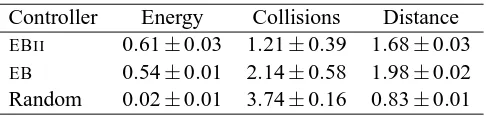
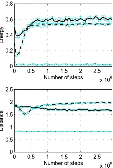
The first set of experiments evaluated theEBIIarchitecture as an alternative toEB. For this purpose three experiments were carried out: one with the EBIIcontroller, one with the EB controller and another with a random controller. The random controller simply selects randomly amongst the differently available behaviors at regular intervals.6 _{The results of this controller can be considered} the baseline performance of the learning controllers. Results are shown in Figure 6 and summarized in Table 3.

Controller Energy Collisions Distance

EBII 0.61±0.03 1.21±0.39 1.68±0.03

EB 0.54±0.01 2.14±0.58 1.98±0.02 Random 0.02±0.01 3.74±0.16 0.83±0.01

Table 3: Summary of the controllers’ performances. The new controller, EBII is compared with its original version, EB. The results of a random controller, which selects random behaviors at regular intervals, are also presented.

Empirically, the EBII controller performs similarly to the EB controller, but with significant statistical differences according to the RANOVA procedure. In fact, it shows a slight improvement in terms of energy and collisions, while maintaining a high distance traveled. Previous exhaustive experiments on the EB controller have shown that it is quite competent and performs better than more traditional approaches (Gadanho and Hallam, 2001b,a, Gadanho, 1999). In fact, previous ex-periments on learning behavior selection using the same adaptive system (Lin, 1993) had to resort to severe simplifications of the behavior selection learning task. These simplifications included having behaviors associated with very specific pre-defined conditions of activation and only interrupting a behavior once it had reached its goal or an inapplicable behavior had become applicable.

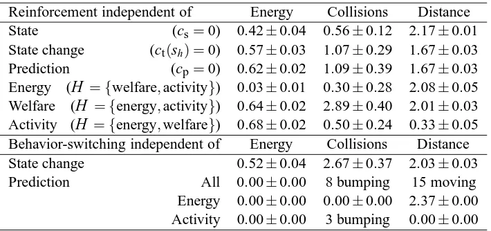
To assess the necessity of each of the properties ofEBII, a new set of experiments was performed for which properties of the controller were removed one at a time for empirical comparison against the complete controller. The results obtained are presented in Table 4.

In terms of reinforcement, the most valuable contribution is that of the state value. Final results obtained without the contributions of state transitions and predictions are very similar to those of the complete controller. Nevertheless, note that these contributions alone, i.e. when the

0 0.5 1 1.5 2 2.5

x 106 0

0.2 0.4 0.6 0.8

Number of steps

Energy

0 0.5 1 1.5 2 2.5

x 106 0

2 4 6

Number of steps

Collisions (%)

0 0.5 1 1.5 2 2.5

x 106 0

0.5 1 1.5 2 2.5

Number of steps

Distance EB version II_EB

Random

Figure 6: EBII compared with the original EB architecture. Results obtained with a random controller provide the baseline of the learning process.

state contribution is omitted, are enough to provide some proficiency in solving the learning task. Furthermore, the omission of these contributions slows learning down, resulting in a larger time to convergence. The decrease in convergence time is larger when the contributions of the state transitions are omitted.

It was also found that for the successful accomplishment of the task and particularly for the achievement of their respective goals, all homeostatic variables should be taken into consideration in the reinforcement. Agents with no energy-dependent reinforcement fail their main task of maintain-ing adequate energy levels. If the welfare contribution is ignored then there is an increased number of collisions. Agents without activity reinforcement move only as a last resort (i.e. when energy is low and there is no light nearby). Avoiding moving helps to reduce the number of collisions.

Reinforcement independent of Energy Collisions Distance

State (cs=0) 0.42±0.04 0.56±0.12 2.17±0.01

State change (ct(sh) =0) 0.57±0.03 1.07±0.29 1.67±0.03

Prediction (cp=0) 0.62±0.02 1.09±0.39 1.67±0.03

Energy (

H

H

H

Behavior-switching independent of Energy Collisions Distance

State change 0.52±0.04 2.67±0.37 2.03±0.03

Prediction All 0.00±0.00 8 bumping 15 moving

Energy 0.00±0.00 0.00±0.00 2.37±0.00 Activity 0.00±0.00 3 bumping 0.00±0.00

Table 4: Summary of results of modifications made to EBII. In the first instance, influences on reinforcement were selectively dropped and in the second instance, specific trigger events were disregarded. In this latter case and in particular if activity prediction events were ignored, the agent would eventually stop receiving triggering events altogether. This would usually happen with the agent stopped in an isolated position, but sometimes it would also happen to a moving agent or to an agent crashed into a wall. These exceptions are accounted for in the table.

5.4.2 ALEC

Three different experiments were carried out, one for each version ofALEC. The difference between version I and version II ofALECrelies on which version of the cognitive system they use, version I and version II respectively. The third version of ALEC will be explained later. In order to analyze the contribution of the two different forms of learning, ALEC version II was submitted to three further experiments: one without cognitive learning (equivalent toEBII, rule acquisition was turned off), one without emotion learning (no learning by the neural-networks in the adaptive system) and one with no learning. The summary of the results obtained can be found in Table 5. This table also repeats the results for theEB controller and presents the results for theLECarchitecture which is discussed later in this section. A summary of the specifications of the different controllers is presented in Table 6.

In Figure 7, the results obtained with first version of ALEC are compared with the results of the EBII architecture. The EBII architecture is presented as the reference since ALEC extends it. These first results show that the addition of a cognitive system provides a significant increase in the learning speed of the agent, but only a very small improvement in terms of reinforcement. In fact, the agent’s performance indicators all converge to better values (the controllers are different according to the RANOVA). The larger differences are in terms of collisions (decrease of near 40%) and distance (increase of almost 20%).

Controller Reinforcement Energy Collisions Distance ALECI 0.22±0.04 0.63±0.03 0.74±0.20 2.00±0.03 ALECII 0.31±0.02 0.69±0.01 0.74±0.35 1.78±0.02 Only emotional learning 0.17±0.04 0.61±0.03 1.21±0.39 1.68±0.03 Only cognitive learning −0.00±0.05 0.48±0.03 0.83±0.38 2.08±0.02 No learning −0.33±0.04 0.25±0.03 1.20±0.16 1.84±0.04 ALECIII — 0.69±0.01 0.55±0.20 1.75±0.02 EB — 0.54±0.01 2.14±0.58 1.98±0.02 LEC −0.50±0.04 0.09±0.03 4.36±0.57 0.78±0.03

Table 5: Summary of the performance of the different versions of the ALECcontroller. Version II was also tested with partial learning abilities (only cognitive or emotional) and with no learning at all. Note that the ALEC controller with no cognitive learning is equivalent to theEBIIpresented earlier. The results obtained with the EB and LEC controllers are also given for comparison.

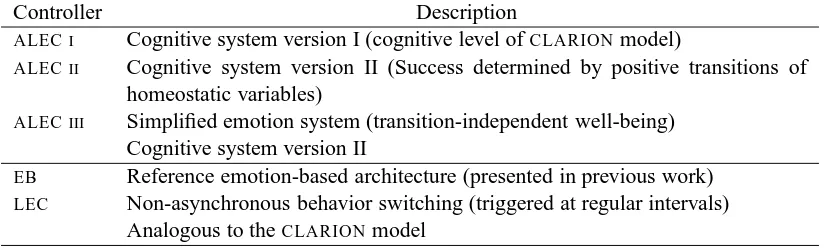
Controller Description

ALECI Cognitive system version I (cognitive level ofCLARIONmodel)

ALECII Cognitive system version II (Success determined by positive transitions of homeostatic variables)

ALECIII Simplified emotion system (transition-independent well-being) Cognitive system version II

EB Reference emotion-based architecture (presented in previous work)

LEC Non-asynchronous behavior switching (triggered at regular intervals)

Analogous to theCLARIONmodel

Table 6: Brief description of the controllers tested.

Analysis of the performance of versions I and II of the cognitive system demonstrates that im-provements in learning are greater when the cognitive system is exclusively dedicated to collecting knowledge about homeostatic variables’ transitions. In fact, the RANOVA procedure showed clear differences in performance between the two versions, with version II achieving higher reinforcement than version I (0.31 against 0.22).

The improvement in performance obtained by the addition of a cognitive system is quite good. This is specially true since theEBarchitecture was designed to solve the exact same task used in the experiments, and has been proved very competent (Gadanho and Hallam, 2001b,a). In this context, a significant improvement in learning speed is already a very good result.

0 0.5 1 1.5 2 2.5

x 106 −0.4

−0.2 0 0.2 0.4

Number of steps

Reinforcement

0 0.5 1 1.5 2 2.5

x 106 0

0.2 0.4 0.6 0.8

Number of steps

Energy

0 0.5 1 1.5 2 2.5

x 106 0

1 2 3

Number of steps

Collisions (%)

0 0.5 1 1.5 2 2.5

x 106 1

1.5 2 2.5

Number of steps

Distance

ALEC version I EB version II

Figure 7: ALECversion I compared with theEBIIarchitecture.

cognitive system does not depend directly on the emotion system. Nevertheless, it is important to recall that the rules of the cognitive system are not meant to cover the full state space and can only predict one trigger step ahead in time. When faced with the task of deciding in every situation, the cognitive system fails.

In the case of theCLARIONmodel, which shares important features with theALECarchitecture, the authors attribute the higher success of the full two-level system to the synergy between the two levels (Sun and Peterson, 1998) which derives from the complementary representations (discrete

vs. continuous) and learning methods (one-shot rule-learning vs. gradual Q-value approximation) of

the two levels. The experimental results obtained with theALEC architecture confirm the success of such a dual approach. The cognitive and emotional system both have serious limitations in their learning abilities — the cognitive system is more accurate but is reduced to a few short-term predictions, while the emotion system provides a broader knowledge which is highly vague and uncertain. However, when working together these limitations are reduced and the robot performance is improved.

0 0.5 1 1.5 2 2.5

x 106 −0.4

−0.2 0 0.2 0.4

Number of steps

Reinforcement

0 0.5 1 1.5 2 2.5

x 106 0

0.2 0.4 0.6 0.8

Number of steps

Energy

0 0.5 1 1.5 2 2.5

x 106 0

1 2 3

Number of steps

Collisions (%)

0 0.5 1 1.5 2 2.5

x 106 1

1.5 2 2.5

Number of steps

Distance

ALEC version II EB version II

Figure 8: ALECversion II compared with theEBIIarchitecture.

The goal system endows ALEC with emotion-like properties and allows it to solve more tasks. In particular, the CLARIONmodel cannot cope with the task used in the experiments presented — experimental results with theLECcontroller confirm that its performance would be compromised by the large number of non-eventful steps. The existence of a goal system also opens extra possibilities for the development of the rule system. For instance, the rule system can be extended to treat separately the various goals of the system and learn how to individually reach the target states of each one of the homeostatic variables. The second version ofALECis an example of how the use of the goal variables can increase the system performance. In this case the rule system specializes in learning about transitions in the agent’s internal variable’s state and leaves long-term state prediction to the emotion system.

0 0.5 1 1.5 2 2.5

x 106 −0.4

−0.2 0 0.2 0.4

Number of steps

Reinforcement

0 0.5 1 1.5 2 2.5

x 106 0

0.2 0.4 0.6 0.8

Number of steps

Energy

0 0.5 1 1.5 2 2.5

x 106 0

1 2 3

Number of steps

Collisions (%)

0 0.5 1 1.5 2 2.5

x 106 1

1.5 2 2.5

Number of steps

Distance

Full Learning Emotional Learning Cognitive Learning No Learning

Figure 9:ALECversion II with different learning abilities on and off.

Furthermore, the results in Figure 10 also show that the full ALEC architecture clearly outper-forms the originalEBarchitecture.

In fact, theALECoutperforms both architectures which inspired it: EBandCLARION.

During the experiments with ALEC and EBII it become apparent that the cognitive system performed better when dedicated to learning state transitions of the homeostatic variables (version II outperformed version I) and that the emotional system still works well when learning only about the state of homeostatic variables (Table 4 shows that state transitions and predictions can be omitted from the reinforcement function). This led to the development of version III of ALEC for which these two roles are divided among the two systems as just discussed. ALECversion III is the same asALECversion II, except that the well-being does not depend on state transitions nor predictions (i.e., ct(sh) =0 and cp=0). Results for this third version are compared with the results of the second version in Figure 11. As expected, although simpler, version III has a performance very similar to version II.7In this new version, the cognitive system is dedicated to tracking individual events which have been significant in terms of major changes in the internal goals of the agent,

0 0.5 1 1.5 2 2.5

x 106 0

0.2 0.4 0.6 0.8

Number of steps

Energy

0 0.5 1 1.5 2 2.5

x 106 0

2 4 6

Number of steps

Collisions (%)

0 0.5 1 1.5 2 2.5

x 106 0

0.5 1 1.5 2 2.5

Number of steps

Distance ALEC version II_EB

LEC

Figure 10:ALEC version II compared with theEBarchitecture and theLECarchitecture.

while the emotion system tries to capture a “feeling” of how good are certain options in terms of long-term internal goal state.

6. Conclusion

The emotion and the cognitive systems ofALEC have distinctive learning capabilities that solve the problem of the overabundance of information provided by the agent-environment interaction in two different ways: one stores all events, but no information to distinguish between individual events, so all events are mixed together; the other one only extracts the most significant events.

TheALECapproach implies that while emotional associations may be more powerful in their ca-pacity to cover states, they lack explanatory power and may introduce errors of over-generalization. Cognitive knowledge, on the other hand, is restricted to learning about simple short-term relations of causality. Cognitive information is more accurate, but at a price — since it is not possible to store and consult all the single events the agent experiences, it selects only the few instances that seem most important.

This is consistent with the idea defended by Cytowic (1993) that emotions give an intuitive sense of what is correct while cognition constructs a model of reality which allow the individual to analyze the decisions.

0 0.5 1 1.5 2 2.5

x 106 0

0.2 0.4 0.6 0.8

Number of steps

Energy

0 0.5 1 1.5 2 2.5

x 106 0

1 2 3

Number of steps

Collisions (%)

0 0.5 1 1.5 2 2.5

x 106 0

0.5 1 1.5 2 2.5

Number of steps

Distance _{ALEC version II}

ALEC version III

Figure 11:ALECversion II compared with version III.

that humans associate high-level cognitive decisions with special feelings that have good or bad connotations depending on whether choices have been emotionally associated with positive or negative long-term outcomes. If these feelings are strong enough, a choice may be immediately followed or discarded. Interestingly, these markers do not have explanatory power and the reason for the selection may not be clear. In fact, although a decision may be reached easily and immediately, the person may subsequently feel the need to use high-level reasoning capabilities to find a reason for the choice. Meanwhile, a fast emotion-based decision could be reached which, depending of the urgency of the situation, may be vital. ALEC shows similar properties when it uses emotional associations to guide the agent. These associations (or more specifically, the utility values) are akin to the somatic-markers suggested by Damasio (1994) in that both provide a long-term indication of the “goodness” of the options available to the agent. Furthermore, the cognitive system can correct the emotion system when it reaches incorrect conclusions. By knowing the exceptions from previous experiences, the cognitive system may choose to override the emotion reactions, which — though powerful — can be more unreliable.

Experimental results have shown that the cognitive system ofALEC can improve learning. The cognitive system cannot perform well without the help of the emotion system because it only has information on part of the state space, but it helps the emotion system to make the correct decisions. The two systems together perform better than either one on its own, suggesting that such a dual approach can be profitable in robotic systems.

The experiments also tested a simple example of how the goal system of ALEC can be used directly by the cognitive system to learn about positive transitions of the agent’s internal state. This proved particularly advantageous in terms of learning performance. This approach relied on the explicit representation of the agent’s goals in terms of homeostatic variables. The representation used consisted of a flat collection of variables and was adequate for the task at hand, but hierarchical structure may be required in order to scale to more complex tasks. Nevertheless, experiments showed how positive transitions of the goal state can be advantageously used in the learning process. Furthermore, experiments showed equivalent performance when the emotion system was dedi-cated solely to the learning of state value, while the cognitive system learned about state changes. This suggests that in a similar hybrid-learning system, the purpose of each learning system may be specialized to address either goal state or goal state transitions and thus simplify the whole system at no cost to the learning performance.

A further advantage ofALECis the infrastructure for endowing the agent with innate knowledge about the world in two distinct forms, as preferences/dislikes in the emotion system or as simple action rules in the cognitive system. For different subproblems of the same task, the knowledge may be more evident to the designer one way or the other.

The fact that ALEC gathers explicit knowledge about the world also opens a door for new future work. Extensions to this architecture could consist of adding more specific knowledge in the cognitive system which then may be used for planning of more complex tasks.

Acknowledgments

The author is a post-doctoral fellow sponsored by the Portuguese Foundation for Science and Technology. This work was partially supported by the FCT Programa Operacional Sociedade de

Informac¸ ˜ao (POSI) in the frame of QCA III. The author thanks Luis Custdio, Nuno Chagas, Rodrigo

Ventura, Brenda Peery, Peter Dayan and the anonymous reviewers for their helpful comments on earlier drafts of this document.

References

James S. Albus. The role of world modeling and value judgment in perception. In A. Meystel, J. Herath, and S. Gray, editors, Proceedings of the 5th _{IEEE International Symposium on}

Intelligent Control. Los Alamitos, CA: IEEE Computer Society Press, 1990.

Minoru Asada. An agent and an environment: A view on body scheme. In Jun Tani and Minoru Asada, editors, Proceedings of the 1996 IROS Workshop on Towards real autonomy, pages 19–24, Senri Life Science Center, Osaka, Japan, 1996.

on Cybernetics and Systems Research, volume 2, pages 745–750, Austria, April 2002. University

of Vienna.

Christian Balkenius. Natural intelligence in artificial creatures. Lund University Cognitive Studies 37, 1995.

Bruce Blumberg. Old Tricks, New Dogs: Ethology and interactive creatures. PhD thesis, MIT, 1996.

Stevo Bozinovski. A self-learning system using secondary reinforcement. In R. Trappl, editor,

Cybernetics and Systems, pages 397–402. Elsevier Science Publishers, North Holland, 1982.

Cynthia Breazeal. Robot in society: Friend or appliance? In Agents’99 workshop on emotion-based

agent architectures, pages 18–26, Seattle, WA, 1999.

Richard E. Cytowic. The man who tasted shapes. Abacus, London, 1993.

Antonio Damasio. The feeling of what happens. Harcout Brace & Company, New York, 1999.

Antonio R. Damasio. Descartes’ error — Emotion, reason and human brain. Picador, London, 1994.

Clark Elliott. The affective reasoner: A process model of emotions in a multi-agent system. PhD thesis, Northwestern University, Evanston, Illinois, 1992. Field of Computer Science.

G´erald Foliot and Olivier Michel. Learning object significance with an emotion based process. In SAB’98 Workshop on Grounding Emotions in Adaptive Systems, pages 25–30, Zurich, Switzerland, 1998.

Masahiro Fujita, Rika Hasegawa, Gabriel Costa, Tsuyoshi Takagi, Jun Yokono, and Hideki Shimomura. Physically and emotionally grounded symbol acquisition for autonomous robots. In Lola Ca˜nmero, editor, AAAI Fall Symposium on Emotional and Intelligent II: The tangled knot

of social cognition, pages 43–48. Menlo Park, California: AAAI Press, 2001. Technical report

FS-01-02.

Sandra Clara Gadanho. Reinforcement Learning in Autonomous Robots: An Empirical Investigation

of the Role of Emotions. PhD thesis, University of Edinburgh, 1999.

Sandra Clara Gadanho and John Hallam. Emotion-triggered learning in autonomous robot control.

Cybernetics and Systems — Special Issue: Grounding emotions in adaptive systems, 32(5):531–

559, July 2001a.

Sandra Clara Gadanho and John Hallam. Robot learning driven by emotions. Adaptive Behavior, 9 (1), 2001b.

Joseph E. LeDoux. The Emotional Brain. Phoenix, London, 1998.

M´arcia Mac¸˜as, Paulo Couto, Carlos Pinto-Ferreira, Luis Cust´odio, and Rodrigo Ventura. Experi-ments with an emotion-based agent using the DARE architecture. In Proceedings of the AISB’01

Symposium on Emotion, Cognition and Affective Computing, pages 105–112, University of York,

U. K., March 2001.

Sridhar Mahadevan and Jonathan Connell. Automatic programming of behavior-based robots using reinforcement learning. Artificial intelligence, 55:311–365, 1992.

Yuval Marom and Gillian Hayes. Maintaining attentional capacity in a social robot. In R. Trappl, editor, Cybernetics and Systems 2000: Proceedings of the 15th European Meeting on Cybernetics

and Systems Research. Symposium on Autonomy Control — Lessons from the emotional,

volume 1, pages 693–698, Vienna, Austria, April 2000.

Maja J. Mataric. Reward functions for accelerated learning. In William W. Cohen and Haym Hirsh, editors, Machine Learning: Proceedings of the Eleventh International Conference, pages 181–189. San Francisco, CA: Morgan Kaufmann Publishers, 1994.

Lee McCauley and Stan Franklin. An architecture for emotion. In Dolores Canamero, editor, AAAI

Fall Symposium on Emotional and Intelligent: The tangled knot of cognition, Technical Report

FS-98-03, pages 122–127. Menlo Park, CA: AAAI Press, 1998.

Olivier Michel. Khepera Simulator package version 2.0: Freeware mobile robot simulator written at the University of Nice Sophia–Antipolis, March 1996. Downloadable from the World Wide

Web athttp://diwww.epfl.ch/lami/team/michel/khep-sim/.

Justus H. Piater, Paul R. Cohen, Xiaoqin Zhang, and Michael Atighetchi. A randomized

ANOVA procedure for comparing performance curves. In J. Shavlik, editor, Machine Learning:

Proceedings of the Fifteenth International Conference, pages 430–438. Morgan Kaufmann

Publishers, San Francisco, CA, 1999.

Miguel Rodriguez and Jean-Pierre Muller. Towards autonomous cognitive animats. In F. Mor´an, A. Moreno, J.J. Merelo, and P. Chac´on, editors, Advances in artificial life — Proceedings of the

Third European Conference on Artificial Life, Lecture Notes in Artificial Intelligence Volume

929, Berlin, Germany, 1995. Springer-Verlag.

Rui Sadio, Gonc¸alo Tavares, Rodrigo Ventura, and Luis Cust´odio. An emotion-based agent architecture application with real robots. In Lola Ca˜nmero, editor, AAAI Fall Symposium on

Emotional and Intelligent II: The tangled knot of social cognition, pages 117–122. Menlo Park,

California: AAAI Press, 2001. Technical report FS-01-02.

Mathias Scheutz. The evolution of simple affective states in multi-agent environments. In Lola Ca˜nmero, editor, Emotional and Intelligent II: The tangled knot of social cognition, pages 123– 128, Menlo Park, California, 2001. AAAI Press. Technical report FS-01-02.

Magy Seif El-Nasr, John Yen, and Thomas Ioerger. Flame - a fuzzy logic adaptive model of emotions. Autonomous Agents and Multi-agent Systems, 1999.

Aaron Sloman and Monica Croucher. Why robots will have emotions. In IJCAI’81 — Proceedings

of the Seventh International Joint Conference on Artificial Intelligence, pages 2369–71, 1981.

Also available as Cognitive Science Research Paper 176, Sussex University.

R. Sun, E. Merrill, and T. Peterson. From implicit skills to explicit knowledge: a bottom-up model of skill learning. Cognitive Science, 25(2):203–244, 2001.

R. Sun and T. Peterson. Autonomous learning of sequential tasks: experiments and analysis. IEEE

Transactions on Neural Networks, 9(6):1217–1234, November 1998.

Richard S. Sutton and Andrew G. Barto. Reinforcement Learning. The MIT Press, 1998.

Silvan S. Tomkins. Affect theory. In Klaus R. Scherer and Paul Ekman, editors, Approaches to

Emotion. Lawrence Erlbaum, London, 1984.

Juan D. Vel´asquez. A computational framework for emotion-based control. In SAB’98 Workshop

on Grounding Emotions in Adaptive Systems, pages 62–67, Zurich, Switzerland, 1998.

Rodrigo Ventura and Carlos Pinto-Ferreira. Emotion-based agents: Three approaches to implemen-tation (preliminary report). In Juan D. Velsquez, editor, Workshop on Emotion-Based Agent

Architectures, Seattle, U. S. A., 1999. Workshop of the Third International Conference on

Autonomous Agents.

C. Watkins. Learning from delayed rewards. PhD thesis, King’s College, Cambridge, 1989.

Ian Wright. Reinforcement learning and animat emotions. In Pattie Maes, Maja J. Mataric, Jean-Arcady Meyer, Jordan Pollack, and Stewart W. Wilson, editors, From animals to animats 4 —

Proceedings of the Fourth International Conference on Simulation of Adaptive Behavior, pages