Tree-Based Batch Mode Reinforcement Learning

Tree-Based Batch Mode Reinforcement Learning

Damien Ernst [email protected]

Pierre Geurts [email protected]

Louis Wehenkel [email protected]

Department of Electrical Engineering and Computer Science Institut Montefiore, University of Li`ege

Sart-Tilman B28 B4000 Li`ege, Belgium

Editor: Michael L. Littman

Abstract

Reinforcement learning aims to determine an optimal control policy from interaction with a system or from observations gathered from a system. In batch mode, it can be achieved by approximating the so-called Q-function based on a set of four-tuples (xt,ut,rt,xt+1)where xt denotes the sys-tem state at time t, ut the control action taken, rt the instantaneous reward obtained and xt+1the successor state of the system, and by determining the control policy from this Q-function. The Q-function approximation may be obtained from the limit of a sequence of (batch mode) super-vised learning problems. Within this framework we describe the use of several classical tree-based supervised learning methods (CART, Kd-tree, tree bagging) and two newly proposed ensemble al-gorithms, namely extremely and totally randomized trees. We study their performances on several examples and find that the ensemble methods based on regression trees perform well in extracting relevant information about the optimal control policy from sets of four-tuples. In particular, the to-tally randomized trees give good results while ensuring the convergence of the sequence, whereas by relaxing the convergence constraint even better accuracy results are provided by the extremely randomized trees.

Keywords: batch mode reinforcement learning, regression trees, ensemble methods, supervised

learning, fitted value iteration, optimal control

1. Introduction

Research in reinforcement learning (RL) aims at designing algorithms by which autonomous agents can learn to behave in some appropriate fashion in some environment, from their interaction with this environment or from observations gathered from the environment (see e.g. Kaelbling et al. (1996) or Sutton and Barto (1998) for a broad overview). The standard RL protocol considers a performance agent operating in discrete time, observing at time t the environment state xt, taking an

action ut, and receiving back information from the environment (the next state xt+1and the

instan-taneous reward rt). After some finite time, the experience the agent has gathered from interaction

with the environment may thus be represented by a set of four-tuples(xt,ut,rt,xt+1).

from this set a control policy which is as close as possible to an optimal policy. Inspired by the on-line Q-learning paradigm (Watkins, 1989), we will approach this batch mode learning problem by computing from the set of four-tuples an approximation of the so-called Q-function defined on the state-action space and by deriving from this latter function the control policy.

When the state and action spaces are finite and small enough, the Q-function can be represented in tabular form, and its approximation (in batch and in on-line mode) as well as the control policy derivation are straightforward. However, when dealing with continuous or very large discrete state and/or action spaces, the Q-function cannot be represented anymore by a table with one entry for each state-action pair. Moreover, in the context of reinforcement learning an approximation of the

Q-function all over the state-action space must be determined from finite and generally very sparse

sets of four-tuples.

To overcome this generalization problem, a particularly attractive framework is the one used by Ormoneit and Sen (2002) which applies the idea of fitted value iteration (Gordon, 1999) to kernel-based reinforcement learning, and reformulates the Q-function determination problem as a sequence of kernel-based regression problems. Actually, this framework makes it possible to take full advan-tage in the context of reinforcement learning of the generalization capabilities of any regression algorithm, and this contrary to stochastic approximation algorithms (Sutton, 1988; Tsitsiklis, 1994) which can only use parametric function approximators (for example, linear combinations of feature vectors or neural networks). In the rest of this paper we will call this framework the fitted Q iteration

algorithm so as to stress the fact that it allows to fit (using a set of four-tuples) any (parametric or

non-parametric) approximation architecture to the Q-function.

The fitted Q iteration algorithm is a batch mode reinforcement learning algorithm which yields an approximation of the Q-function corresponding to an infinite horizon optimal control problem with discounted rewards, by iteratively extending the optimization horizon (Ernst et al., 2003):

• At the first iteration it produces an approximation of a Q1-function corresponding to a 1-step

optimization. Since the true Q1-function is the conditional expectation of the instantaneous

reward given the state-action pair (i.e., Q1(x,u) =E[rt|xt =x,ut =u]), an approximation of

it can be constructed by applying a (batch mode) regression algorithm to a training set whose inputs are the pairs(xt,ut) and whose target output values are the instantaneous rewards rt

(i.e., q1,t=rt).

• The Nth iteration derives (using a batch mode regression algorithm) an approximation of a

QN-function corresponding to an N-step optimization horizon. The training set at this step

is obtained by merely refreshing the output values of the training set of the previous step by

using the “value iteration” based on the approximate QN-function returned at the previous

step (i.e., qN,t=rt+γmaxuQˆN−1(xt+1,u), whereγ∈[0,1)is the discount factor).

Ormoneit and Sen (2002) have studied the theoretical convergence and consistency properties of this algorithm when combined with kernel-based regressors. In this paper, we study within this framework the empirical properties and performances of several tree-based regression algorithms on several applications. Just like kernel-based methods, tree-based methods are non-parametric and offer a great modeling flexibility, which is a paramount characteristic for the framework to be

successful since the regression algorithm must be able to model any QN-function of the sequence,

efficiency and scalability to high-dimensional spaces, their fully autonomous character, and their recognized robustness to irrelevant variables, outliers, and noise.

In addition to good accuracy when trained with finite sets of four-tuples, one desirable feature of the regression method used in the context of the fitted Q iteration algorithm is to ensure convergence of the sequence. We will analyze under which conditions the tree-based methods share this property and also what is the relation between convergence and quality of approximation. In particular, we will see that ensembles of totally randomized trees (i.e., trees built by selecting their splits randomly) can be adapted to ensure the convergence of the sequence while leading to good approximation performances. On the other hand, another tree-based algorithm named extremely randomized trees (Geurts et al., 2004), will be found to perform consistently better than totally randomized trees even though it does not strictly ensure the convergence of the sequence of Q-function approximations.

The remainder of this paper is organized as follows. In Section 2, we formalize the reinforce-ment learning problem considered here and recall some classical results from optimal control theory upon which the approach is based. In Section 3 we present the fitted Q iteration algorithm and in Section 4 we describe the different tree-based regression methods considered in our empirical tests. Section 5 is dedicated to the experiments where we apply the fitted Q iteration algorithm used with tree-based methods to several control problems with continuous state spaces and evaluate its perfor-mances in a wide range of conditions. Section 6 concludes and also provides our main directions for further research. Three appendices collect relevant details about algorithms, mathematical proofs and benchmark control problems.

2. Problem Formulation and Dynamic Programming

We consider a time-invariant stochastic system in discrete time for which a closed loop stationary control policy1must be chosen in order to maximize an expected discounted return over an infinite time horizon. We formulate hereafter the batch mode reinforcement learning problem in this context and we restate some classical results stemming from Bellman’s dynamic programming approach to optimal control theory (introduced in Bellman, 1957) and from which the fitted Q iteration algorithm takes its roots.

2.1 Batch Mode Reinforcement Learning Problem Formulation

Let us consider a system having a discrete-time dynamics described by

xt+1= f(xt,ut,wt) t=0,1,···, (1)

where for all t, the state xt is an element of the state space X , the action utis an element of the action

space U and the random disturbance wt an element of the disturbance space W . The disturbance wt

is generated by the time-invariant conditional probability distribution Pw(w_|x,u).2

To the transition from t to t+1 is associated an instantaneous reward signal rt =r(xt,ut,wt)

where r(x,u,w)is the reward function supposed to be bounded by some constant Br.

Let µ(_·): X _→U denote a stationary control policy and J_∞µ denote the expected return ob-tained over an infinite time horizon when the system is controlled using this policy (i.e., when

1. Indeed, in terms of optimality this restricted family of control policies is as good as the broader set of all non-anticipating (and possibly time-variant) control policies.

2. In other words, the probability P(wt=w|xt=x,ut=u)of occurrence of wt=w given that the current state xt and

ut=µ(xt),∀t). For a given initial condition x0=x, J_∞µ is defined by

J_∞µ(x) = lim

N→∞ Ewt t=0,1,···,N−1

[ N₋1

∑

t=0 γt_r(x

t,µ(xt),wt)|x0=x], (2)

whereγis a discount factor (0_≤γ<1) that weights short-term rewards more than long-term ones, and where the conditional expectation is taken over all trajectories starting with the initial condi-tion x0=x. Our objective is to find an optimal stationary policy µ∗, i.e. a stationary policy that

maximizes J_∞µ for all x.

The existence of an optimal stationary closed loop policy is a classical result from dynamic programming theory. It could be determined in principle by solving the Bellman equation (see below, Eqn (6)) given the knowledge of the system dynamics and reward function. However, the sole information that we assume available to solve the problem is the one obtained from the observation of a certain number of one-step system transitions (from t to t+1). Each system transition provides the knowledge of a new four-tuple(xt,ut,rt,xt+1) of information. Since, except for very special

conditions, it is not possible to determine exactly an optimal control policy from a finite sample of such transitions, we aim at computing an approximation of such a µ∗from a set

F

F

of such four-tuples.

We do not make any particular assumptions on the way the set of four-tuples is generated. It could be generated by gathering the four-tuples corresponding to one single trajectory (or episode) as well as by considering several independently generated one or multi-step episodes.

We call this problem the batch mode reinforcement learning problem because the algorithm is allowed to use a set of transitions of arbitrary size to produce its control policy in a single step. In contrast, an on-line algorithm would produce a sequence of policies corresponding to a sequence of four-tuples.

2.2 Results from Dynamic Programming Theory

For a temporal horizon of N steps, let us denote by

πN(t,x)∈U,t∈ {0,···,N−1}; x∈X

a (possibly time-varying) N-step control policy (i.e., ut=πN(t,xt)), and by

J_NπN(x) = E

wt t=0,1,···,N−1

[ N−1

∑

t=0 γt_r(x

t,πN(t,xt),wt)|x0=x] (3)

its expected return over N steps. An N-step optimal policyπ∗_N is a policy which among all possible such policies maximizes J_NπNfor any x. Notice that under mild conditions (see e.g. Hern´andez-Lerma and Lasserre, 1996, for the detailed conditions) such a policy always does indeed exist although it is not necessarily unique.

1. The sequence of QN-functions defined on X×U by

Q0(x,u) ≡ 0 (4)

QN(x,u) = (HQN₋1)(x,u), ∀N>0, (5)

converges (in infinity norm) to the Q-function, defined as the (unique) solution of the Bellman equation:

Q(x,u) = (HQ)(x,u) (6)

where H is an operator mapping any function K : X_×U_→R_{and defined as follows:}3

(HK)(x,u) = E

w[r(x,u,w) +γmaxu0_∈UK(f(x,u,w),u

0_{)]. (7)}

Uniqueness of solution of Eqn (6) as well as convergence of the sequence of QN-functions

to this solution are direct consequences of the fixed point theorem and of the fact that H is a contraction mapping.

2. The sequence of policies defined by the two conditions4

π∗

N(0,x) = arg max u0_∈U QN(x

,u0),∀N>0 (8)

π∗

N(t+1,x) = π∗N−1(t,x),∀N>1,t∈ {0, . . . ,N−2} (9)

are N-step optimal policies, and their expected returns over N steps are given by

Jπ∗N

N (x) =max_u

∈UQN(x,u).

3. A policy µ∗that satisfies

µ∗(x) =arg max

u_∈U

Q(x,u) (10)

is an optimal stationary policy for the infinite horizon case and the expected return of µ∗_N(x)=. π∗

N(0,x)converges to the expected return of µ∗:

lim

N_→∞J µ∗N

∞ (x) =J_∞µ∗(x) _∀x_∈X. (11)

We have also limN_→∞Jπ ∗ N

N (x) =Jµ ∗

∞(x) ∀x∈X .

Equation (5) defines the so-called value iteration algorithm5 providing a way to determine

iter-atively a sequence of functions converging to the Q-function and hence of policies whose return converges to that of an optimal stationary policy, assuming that the system dynamics, the reward function and the noise distribution are known. As we will see in the next section, it suggests also a

way to determine approximations of these QN-functions and policies from a sample

F

3. The expectation is computed by using P(w) =Pw(w|x,u).

4. Actually this definition does not necessarily yield a unique policy, but any policy which satisfies these conditions is appropriate.

5. Strictly, the term “value iteration” refers to the computation of the value function J_∞µ∗and corresponds to the iteration Jπ∗N

N =max_u

∈UEw[r(x,u,w) +γJ π∗

N−1

3. Fitted Q Iteration Algorithm

In this section, we introduce the fitted Q iteration algorithm which computes from a set of four-tuples an approximation of the optimal stationary policy.

3.1 The Algorithm

A tabular version of the fitted Q iteration algorithm is given in Figure 1. At each step this algorithm may use the full set of four-tuples gathered from observation of the system together with the function computed at the previous step to determine a new training set which is used by a supervised learning (regression) method to compute the next function of the sequence. It produces a sequence of ˆQN

-functions, approximations of the QN-functions defined by Eqn (5).

Inputs: a set of four-tuples

F

Initialization:

Set N to 0 .

Let ˆQNbe a function equal to zero everywhere on X×U .

Iterations:

Repeat until stopping conditions are reached

- N_←N+1 .

- Build the training set

T S

F

the full set of four-tuples

F

il = (xl_t,u_tl), (12)

ol = r_tl+γmax

u_∈U

ˆ

QN−1(xt+1l ,u). (13)

- Use the regression algorithm to induce from

T S

Figure 1: Fitted Q iteration algorithm

Notice that at the first iteration the fitted Q iteration algorithm is used in order to produce an approximation of the expected reward Q1(x,u) =Ew[r(x,u,w)]. Therefore, the considered training set uses input/output pairs (denoted(il,ol)) where the inputs are the state-action pairs and the outputs the observed rewards. In the subsequent iterations, only the output values of these input/output pairs are updated using the value iteration based on the ˆQN-function produced at the preceding step and

information about the reward and the successor state reached in each tuple.

It is important to realize that the successive calls to the supervised learning algorithm are totally independent. Hence, at each step it is possible to adapt the resolution (or complexity) of the learned model so as to reach the best bias/variance tradeoff at this step, given the available sample.

3.2 Algorithm Motivation

xt+1= f(xt,ut)and rt =r(xt,ut)and Eqn (5) may be rewritten

QN(x,u) =r(x,u) +γmax

u0_∈UQN−1(f(x,u),u

0_{). (14)}

If we suppose that the function QN−1is known, we can use this latter equation and the set of

four-tuples

F

F

We have indeed QN(xtl,utl) =rtl+γmax u0_∈UQN−1(x

l

t+1,u0), since xlt+1= f(xlt,utl)and rtl=r(xlt,ult).

We can thus build a training set

T S

F

algorithm in order to generalize this information to any unseen state-action pair or, stated in another way, to fit a function approximator to this training set in order to get an approximation ˆQNof QNover

the whole state-action space. If we substitute ˆQN for QN we can, by applying the same reasoning,

determine iteratively ˆQN+1, ˆQN+2, etc.

In the stochastic case, the evaluation of the right hand side of Eqn (14) for some four-tuples

(xt,ut,rt,xt+1) is no longer equal to QN(xt,ut) but rather is the realization of a random variable

whose expectation is QN(xt,ut). Nevertheless, since a regression algorithm usually6 seeks an

ap-proximation of the conditional expectation of the output variable given the inputs, its application to the training set

T S

space.

3.3 Stopping Conditions

The stopping conditions are required to decide at which iteration (i.e., for which value of N) the process can be stopped. A simple way to stop the process is to define a priori a maximum number of iterations. This can be done for example by noting that for a sequence of optimal policies µ∗_N, an error bound on the sub-optimality in terms of number of iterations is given by the following equation

kJµ∗N

∞ −J_∞µ∗_k∞≤2 γ

N_B r

(1₋γ)2. (15)

Given the value of Br and a desired level of accuracy, one can then fix the maximum number of

iterations by computing the minimum value of N such that the right hand side of this equation is smaller than the tolerance fixed.7

Another possibility would be to stop the iterative process when the distance between ˆQN and

ˆ

QN−1drops below a certain value. Unfortunately, for some supervised learning algorithms there is

no guarantee that the sequence of ˆQN-functions actually converges and hence this kind of

conver-gence criterion does not necessarily make sense in practice.

3.4 Control Policy Derivation

When the stopping conditions - whatever they are - are reached, the final control policy, seen as an approximation of the optimal stationary closed loop control policy is derived by

ˆµ∗_N(x) =arg max

u∈U

ˆ

QN(x,u). (16)

6. This is true in the case of least squares regression, i.e. in the vast majority of regression methods.

7. Equation (15) gives an upper bound on the suboptimality of µ∗_N and not of ˆµ∗_N. By exploiting this upper bound to determine a maximum number of iterations, we assume implicitly that ˆµ∗_N is a good approximation of µ∗_N(that

kJˆµ∗N

∞ −Jµ∗N

When the action space is discrete, it is possible to compute the value ˆQN(x,u)for each value

of u and then find the maximum. Nevertheless, in our experiments we have sometimes adopted a different approach to handle discrete action spaces. It consists of splitting the training samples according to the value of u and of building the approximation ˆQN(x,u) by separately calling for

each value of u_∈U the regression method on the corresponding subsample. In other words, each

such model is induced from the subset of four-tuples whose value of the action is u, i.e.

F

F

At the end, the action at some point x of the state space is computed by applying to this state each model ˆQN(x,u),u∈U and looking for the value of u yielding the highest value.

When the action space is continuous, it may be difficult to compute the maximum especially because we can not make any a priori assumption about the shape of the Q-function (e.g. convex-ity). However, taking into account particularities of the models learned by a particular supervised learning method, it may be more or less easy to compute this value (see Section 4.5 for the case of tree-based models).

3.5 Convergence of the Fitted Q Iteration Algorithm

The fitted Q iteration algorithm is said to converge if there exists a function ˆQ : X_×U _→R_such

that_∀ε>0 there exists a n∈Nsuch that:

k_Qˆ_N−Qˆ_{k∞<ε ∀N>n.}

Convergence may be ensured if we use a supervised learning method which given a sample

T S

{(i1,o1), . . . ,(i#T S,o#T S)_}produces at each call the model (proof in Appendix B):

f(i) =

#T S

∑

l=1

kT S(il,i)∗ol, (17)

with the kernel kT S(il,i) being the same from one call to the other within the fitted Q iteration algorithm8and satisfying the normalizing condition:

#T S

∑

l=1

|kT S(il,i)|=1,∀i. (18)

Supervised learning methods satisfying these conditions are for example the k-nearest-neighbors method, partition and multi-partition methods, locally weighted averaging, linear, and multi-linear interpolation. They are collectively referred to as kernel-based methods (see Gordon, 1999; Or-moneit and Sen, 2002).

3.6 Related Work

As stated in the Introduction, the idea of trying to approximate the Q-function from a set of four-tuples by solving a sequence of supervised learning problems may already be found in Ormoneit and

Sen (2002). This work however focuses on kernel-based methods for which it provides convergence and consistency proofs, as well as a bias-variance characterization. While in our formulation state and action spaces are handled in a symmetric way and may both be continuous or discrete, in their work Ormoneit and Sen consider only discrete action spaces and use a separate kernel for each value of the action.

The work of Ormoneit and Sen is related to earlier work aimed to solve large-scale dynamic pro-gramming problems (see for example Bellman et al., 1973; Gordon, 1995b; Tsitsiklis and Van Roy, 1996; Rust, 1997). The main difference is that in these works the various elements that compose the optimal control problem are supposed to be known. We gave the name fitted Q iteration to our algorithm given in Figure 1 to emphasize that it is a reinforcement learning version of the fitted

value iteration algorithm whose description may be found in Gordon (1999). Both algorithms are

quite similar except that Gordon supposes that a complete generative model is available,9 which is a rather strong restriction with respect to the assumptions of the present paper.

In his work, Gordon characterizes a class of supervised learning methods referred to as averagers that lead to convergence of his algorithm. These averagers are in fact a particular family of kernels as considered by Ormoneit and Sen. In Boyan and Moore (1995), serious convergence problems that may plague the fitted value iteration algorithm when used with polynomial regression, back-propagation, or locally weighted regression are shown and these also apply to the reinforcement learning context. In their paper, Boyan and Moore propose also a way to overcome this problem by relying on some kind of Monte-Carlo simulations. In Gordon (1995a) and Singh et al. (1995) on-line versions of the fitted value iteration algorithm used with averagers are presented.

In Moore and Atkeson (1993) and Ernst (2003), several reinforcement learning algorithms closely related to the fitted Q iteration algorithm are given. These algorithms, known as model-based algorithms, build explicitly from the set of observations a finite Markov Decision Process (MDP) whose solution is then used to adjust the parameters of the approximation architecture used to represent the Q-function. When the states of the MDP correspond to a finite partition of the original state space, it can be shown that these methods are strictly equivalent to using the fitted Q iteration algorithm with a regression method which consists of simply averaging the output values of the training samples belonging to a given cell of the partition.

In Boyan (2002), the Least-Squares Temporal-Difference (LSTD) algorithm is proposed. This algorithm uses linear approximation architectures and learns the expected return of a policy. It is similar to the fitted Q iteration algorithm combined with linear regression techniques on problems for which the action space is composed of a single element. Lagoudakis and Parr (2003a) intro-duce the Least-Squares Policy Iteration (LSPI) which is an extension of LSTD to control problems. The model-based algorithms in Ernst (2003) that consider representative states as approximation architecture may equally be seen as an extension of LSTD to control problems.

Finally, we would like to mention some recent works based on the idea of reductions of rein-forcement learning to supervised learning (classification or regression) with various assumptions concerning the available a priori knowledge (see e.g. Kakade and Langford, 2002; Langford and Zadrozny, 2004, and the references therein). For example, assuming that a generative model is available,10 an approach to solve the optimal control problem by reformulating it as a sequence of 9. Gordon supposes that the functions f(·,·,·), r(·,·,·), and Pw(·|·,·)are known and considers training sets composed of

elements of the type(x,max

u_∈UEw[r(x,u,w) +γ

ˆ Jπ∗N−1

N−1(f(x,u,w))]).

standard supervised classification problems has been developed (see Lagoudakis and Parr, 2003b; Bagnell et al., 2003), taking its roots from the policy iteration algorithm, another classical dynamic programming algorithm. Within this “reductionist” framework, the fitted Q iteration algorithm can be considered as a reduction of reinforcement learning to a sequence of regression tasks, inspired by the value iteration algorithm and usable in the rather broad context where the available information is given in the form of a set of four-tuples. This batch mode context incorporates indeed both the on-line context (since one can always store data gathered on-line, at least for a finite time interval) as well as the generative context (since one can always use the generative model to generate a sample of four-tuples) as particular cases.

4. Tree-Based Methods

We will consider in our experiments five different tree-based methods all based on the same top-down approach as in the classical tree induction algorithm. Some of these methods will produce from the training set a model composed of one single regression tree while the others build an

en-semble of regression trees. We characterize first the models that will be produced by these tree-based

methods and then explain how the different tree-based methods generate these models. Finally, we will consider some specific aspects related to the use of tree-based methods with the fitted Q itera-tion algorithm.

4.1 Characterization of the Models Produced

A regression tree partitions the input space into several regions and determines a constant prediction in each region of the partition by averaging the output values of the elements of the training set

T S

which belong to this region. Let S(i)be the function that assigns to an input i (i.e., a state-action pair) the region of the partition it belongs to. A regression tree produces a model that can be described by Eqn (17) with the kernel defined by the expression:

kT S(il,i) =

IS(i)(il)

∑(a,b)∈T SIS(i)(a)

(19)

where IB(·)denotes the characteristic function of the region B (IB(i) =1 if i∈B and 0 otherwise).

When a tree-based method builds an ensemble of regression trees, the model it produces av-erages the predictions of the different regression trees to make a final prediction. Suppose that a

tree-based ensemble method produces p regression trees and gets as input a training set

T S

T S

Sm(i)be the function that assigns to each i the region of the mth partition it belongs to. The model

produced by the tree-based method may also be described by Eqn (17) with the kernel defined now by the expression:

kT S(il,i) =

1

p

p

∑

m=1

ISm(i)(i

l₎ ∑(a,b)∈T SmISm(i)(a)

. (20)

It should also be noticed that kernels (19) and (20) satisfy the normalizing condition (18).

4.2 The Different Tree-Based Algorithms

All the tree induction algorithms that we consider are top-down in the sense that they create their partition by starting with a single subset and progressively refining it by splitting its subsets into pieces. The tree-based algorithms that we consider differ by the number of regression trees they build (one or an ensemble), the way they grow a tree from a training set (i.e., the way the different tests inside the tree are chosen) and, in the case of methods that produce an ensemble of regression trees, also the way they derive from the original training set

T S

T S

left else go right” where ij represents the jth input (or jth attribute) of the input vector i. In what

follows the split variables t and ij are referred to as the cut-point and the cut-direction (or attribute)

of the split (or test)[ij<t].

We now describe the tree-based regression algorithms used in this paper.

4.2.1 KD-TREE

In this method the regression tree is built from the training set by choosing the cut-point at the local median of the cut-direction so that the tree partitions the local training set into two subsets of the same cardinality. The cut-directions alternate from one node to the other: if the direction of cut is

ij for the parent node, it is equal to ij+1for the two children nodes if j+1<n with n the number

of possible cut-directions and i1 otherwise. A node is a leaf (i.e., is not partitioned) if the training

sample corresponding to this node contains less than nmintuples. In this method the tree structure is

independent of the output values of the training sample, i.e. it does not change from one iteration to another of the fitted Q iteration algorithm.

4.2.2 PRUNEDCART TREE

The classical CART algorithm is used to grow completely the tree from the training set (Breiman et al., 1984). This algorithm selects at a node the test (i.e., the cut-direction and cut-point) that maximizes the average variance reduction of the output variable (see Eqn (25) in Appendix A). The tree is pruned according to the cost-complexity pruning algorithm with error estimate by ten-fold cross validation. Because of the score maximization and the post-pruning, the tree structure depends on the output values of the training sample; hence, it may change from one iteration to another.

4.2.3 TREEBAGGING

We refer here to the standard algorithm published by Breiman (1996). An ensemble of M trees is built. Each tree of the ensemble is grown from a training set by first creating a bootstrap replica (random sampling with replacement of the same number of elements) of the training set and then building an unpruned CART tree using that replica. Compared to the Pruned CART Tree algorithm, Tree Bagging often improves dramatically the accuracy of the model produced by reducing its variance but increases the computing times significantly. Note that during the tree building we also stop splitting a node if the number of training samples in this node is less than nmin. This algorithm

One single regression tree is built

An ensemble of regression trees is built Tests do depend on the output

values (o) of the(i,o)∈T S CART

Tree Bagging Extra-Trees Tests do not depend on the output

values (o) of the(i,o)∈T S Kd-Tree Totally Randomized Trees

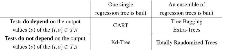
Table 1: Main characteristics of the different tree-based algorithms used in the experiments.

4.2.4 EXTRA-TREES

Besides Tree Bagging, several other methods to build tree ensembles have been proposed that often improve the accuracy with respect to Tree Bagging (e.g. Random Forests, Breiman, 2001). In this paper, we evaluate our recently developed algorithm that we call “Extra-Trees”, for extremely randomized trees (Geurts et al., 2004). Like Tree Bagging, this algorithm works by building several (M) trees. However, contrary to Tree Bagging which uses the standard CART algorithm to derive the trees from a bootstrap sample, in the case of Extra-Trees, each tree is built from the complete original training set. To determine a test at a node, this algorithm selects K cut-directions at random and for each cut-direction, a cut-point at random. It then computes a score for each of the K tests and chooses among these K tests the one that maximizes the score. Again, the algorithm stops splitting a node when the number of elements in this node is less than a parameter nmin. Three parameters are

associated to this algorithm: the number M of trees to build, the number K of candidate tests at each node and the minimal leaf size nmin. The detailed tree building procedure is given in Appendix A.

4.2.5 TOTALLYRANDOMIZEDTREES

Totally Randomized Trees corresponds to the case of Extra-Trees when the parameter K is chosen equal to one. Indeed, in this case the tests at the different nodes are chosen totally randomly and independently from the output values of the elements of the training set. Actually, this algorithm is equivalent to an algorithm that would build the tree structure totally at random without even looking at the training set and then use the training set only to remove the tests that lead to empty branches and decide when to stop the development of a branch (Geurts et al., 2004). This algorithm can therefore be degenerated in the context of the usage that we make of it in this paper by freezing the tree structure after the first iteration, just as the Kd-Trees.

4.2.6 DISCUSSION

Table 1 classifies the different tree-based algorithms considered according to two criteria: whether they build one single or an ensemble of regression trees and whether the tests computed in the trees depend on the output values of the elements of the training set. We will see in the experiments that these two criteria often characterize the results obtained.

For the Extra-Trees, experiments in Geurts et al. (2004) have shown that a good default value for the parameter K in regression is actually the dimension of the input space. In all our experiments,

K will be set to this default value.

While pruning generally improves significantly the accuracy of single regression trees, in the context of ensemble methods it is commonly admitted that unpruned trees are better. This is sug-gested from the bias/variance tradeoff, more specifically because pruning reduces variance but in-creases bias and since ensemble methods reduce very much the variance without increasing too much bias, there is often no need for pruning trees in the context of ensemble methods. However, in high-noise conditions, pruning may be useful even with ensemble methods. Therefore, we will use a cross-validation approach to automatically determine the value of nminin the context of ensemble

methods. In this case, pruning is carried out by selecting at random two thirds of the elements of

T S

value of nmin the ensemble minimizes the square error over the last third of the elements. Then,

the ensemble method is run again on the whole training set using this value of nminto produce the

final model. In our experiments, the resulting algorithm will have the same name as the original ensemble method preceded by the term Pruned (e.g. Pruned Tree Bagging). The same approach will also be used to prune Kd-Trees.

4.3 Convergence of the Fitted Q Iteration Algorithm

Since the models produced by the tree-based methods may be described by an expression of the type (17) with the kernel kT S(il,i)satisfying the normalizing condition (18), convergence of the fitted Q iteration algorithm can be ensured if the kernel kT S(il,i)remains the same from one iteration to the other. This latter condition is satisfied when the tree structures remain unchanged throughout the different iterations.

For the Kd-Tree algorithm which selects tests independently of the output values of the elements of the training set, it can be readily seen that it will produce at each iteration the same tree structure if the minimum number of elements to split a leaf (nmin) is kept constant. This also implies that the

tree structure has just to be built at the first iteration and that in the subsequent iterations, only the values of the terminal leaves have to be refreshed. Refreshment may be done by propagating all the elements of the new training set in the tree structure and associating to a terminal leaf the average output value of the elements having reached this leaf.

For the totally randomized trees, the tests do not depend either on the output values of the elements of the training set but the algorithm being non-deterministic, it will not produce the same tree structures at each call even if the training set and the minimum number of elements (nmin) to

split a leaf are kept constant. However, since the tree structures are independent from the output, it is not necessary to refresh them from one iteration to the other. Hence, in our experiments, we will build the set of totally randomized trees only at the first iteration and then only refresh predictions at terminal nodes at subsequent iterations. The tree structures are therefore kept constant from one iteration to the other and this will ensure convergence.

4.4 No Divergence to Infinity

We say that the sequence of functions ˆQNdiverges to infinity if lim N→∞k

ˆ

QNk∞→∞.

depend on the output values (o) of the input-output pairs ((i,o)), the sequence of ˆQN-functions

remains bounded. Indeed, the prediction value of a leaf being the average value of the outputs of the elements of the training set that correspond to this leaf, we have_kQˆN(x,u)k∞≤Br+γkQˆN−1(x,u)k∞

where Br is the bound of the rewards. And, since ˆQ0(x,u) =0 everywhere, we therefore have

kQˆN(x,u)_k∞≤ Br

1−γ ∀N∈N.

However, we have observed in our experiments that for some other supervised learning meth-ods, divergence to infinity problems were plaguing the fitted Q iteration algorithm (Section 5.3.3); such problems have already been highlighted in the context of approximate dynamic programming (Boyan and Moore, 1995).

4.5 Computation of maxu∈UQˆN(x,u)when u Continuous

In the case of a single regression tree, ˆQN(x,u)is a piecewise-constant function of its argument u, when fixing the state value x. Thus, to determine max

u∈U

ˆ

QN(x,u),it is sufficient to compute the value

of ˆQN(x,u)for a finite number of values of U , one in each hyperrectangle delimited by the values

of discretization thresholds found in the tree.

The same argument can be extended to ensembles of regression trees. However, in this case, the number of discretization thresholds might be much higher and this resolution scheme might become computationally inefficient.

5. Experiments

Before discussing our simulation results, we first give an overview of our test problems, of the type of experiments carried out and of the different metrics used to assess the performances of the algorithms.

5.1 Overview

We consider five different problems, and for each of them we use the fitted Q iteration algorithm with the tree-based methods described in Section 4 and assess their ability to extract from different sets of four-tuples information about the optimal control policy.

5.1.1 TESTPROBLEMS

The first problem, referred to as the “Left or Right” control problem, has a one-dimensional state space and a stochastic dynamics. Performances of tree-based methods are illustrated and compared with grid-based methods.

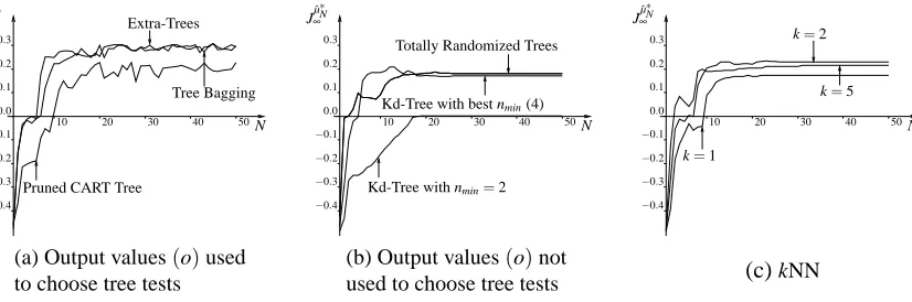
Next we consider the “Car on the Hill” test problem. Here we compare our algorithms in depth with other methods (k-nearest-neighbors, grid-based methods, a gradient version of the on-line Q-learning algorithm) in terms of accuracy and convergence properties. We also discuss CPU considerations, analyze the influence of the number of trees built on the solution, and the effect of irrelevant state variables and continuous action spaces.

The third problem is the “Acrobot Swing Up” control problem. It is a four-dimensional and de-terministic control problem. While in the first two problems the four-tuples are generated randomly

prior to learning, here we consider the case where the estimate of µ∗ deduced from the available

The two last problems (“Bicycle Balancing” and “Bicycle Balancing and Riding”) are treated together since they differ only in their reward function. They have a stochastic dynamics, a seven-dimensional state space and a two-seven-dimensional control space. Here we look at the capability of our method to handle rather challenging problems.

5.1.2 METRICS TOASSESS PERFORMANCES OF THE ALGORITHMS

In our experiments, we will use the fitted Q iteration algorithm with several types of supervised

learning methods as well as other algorithms like Q-learning or Watkin’s Q(λ) with various

ap-proximation architectures. To rank performances of the various algorithms, we need to define some metrics to measure the quality of the solution they produce. Hereafter we review the different met-rics considered in this paper.

Expected return of a policy. To measure the quality of a solution given by a RL algorithm, we can

use the stationary policy it produces, compute the expected return of this stationary policy and say that the higher this expected return is, the better the RL algorithm performs. Rather than computing the expected return for one single initial state, we define in our examples a set of initial states named

Xi, chosen independently from the set of four-tuples

F

score of µ= ∑x∈XiJ µ ∞(x)

#Xi (21)

To evaluate this expression, we estimate, for every initial state x_∈Xi_{, J}µ

∞(x)by Monte-Carlo

sim-ulations. If the control problem is deterministic, one simulation is enough to estimate J_∞µ(x). If the control problem is stochastic, several simulations are carried out. For the “Left or Right” control

problem, 100,000 simulations are considered. For the “Bicycle Balancing” and “Bicycle Balancing

and Riding” problems, whose dynamics is less stochastic and Monte-Carlo simulations computa-tionally more demanding, 10 simulations are done. For the sake of compactness, the score of µ is represented in the figures by J_∞µ.

Fulfillment of a specific task. The score of a policy assesses the quality of a policy through its

expected return. In the “Bicycle Balancing” control problem, we also assess the quality of a policy through its ability to avoid crashing the bicycle during a certain period of time. Similarly, for the “Bicycle Balancing and Riding” control problem, we consider a criterion of the type “How often does the policy manage to drive the bicycle, within a certain period of time, to a goal ?”.

Bellman residual. While the two previous metrics were relying on the policy produced by the

RL algorithm, the metric described here relies on the approximate Q-function computed by the RL algorithm. For a given function ˆQ and a given state-action pair(x,u), the Bellman residual is defined to be the difference between the two sides of the Bellman equation (Baird, 1995), the Q-function being the only Q-function leading to a zero Bellman residual for every state-action pair. In our simulation, to estimate the quality of a function ˆQ, we exploit the Bellman residual concept by

associating to ˆQ the mean square of the Bellman residual over the set Xi_×U , value that will be

referred to as the Bellman residual of ˆQ. We have

Bellman residual of ˆQ= ∑(x,u)∈Xi×U(

ˆ

Q(x,u)₋(H ˆQ)(x,u))2

xt

ut+wt

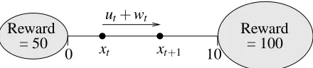
Reward Reward

xt+1 = 100

= 50

0 10

Figure 2: The “Left or Right” control problem.

This metric is only used in the “Left or Right” control problem to compare the quality of the solu-tions obtained. A metric relying on the score is not discriminant enough for this control problem, since all the algorithms considered can easily learn a good approximation of the optimal stationary policy. Furthermore, for this control problem, the term(H ˆQ)(x,u)in the right side of Eqn (22) is estimated by drawing independently and for each(x,u)_∈Xi_×U , 100,000 values of w according to Pw(.|x,u)(see Eqn (7)).

In the figures, the Bellman residual of ˆQ is represented by d(_Qˆ_{,H ˆQ).}

5.2 The “Left or Right” Control Problem

We consider here the “Left or Right” optimal control problem whose precise definition is given in Appendix C.1.

The main characteristics of the control problem are represented on Figure 2. A point travels in the interval[0,10]. Two control actions are possible. One tends to drive the point to the right (u=2) while the other to the left (u=₋2). As long as the point stays inside the interval, only zero rewards are observed. When the point leaves the interval, a terminal state12is reached. If the point goes out on the right side then a reward of 100 is obtained while it is twice less if it goes out on the left.

Even if going out on the right may finally lead to a better reward, µ∗is not necessarily equal to 2 everywhere since the importance of the reward signal obtained after t steps is weighted by a factor

γ(t−1)₌₀

.75(t−1).

5.2.1 FOUR-TUPLES GENERATION

To collect the four-tuples we observe 300 episodes of the system. Each episode starts from an initial state chosen at random in[0,10]and finishes when a terminal state is reached. During the episodes, the action ut selected at time t is chosen at random with equal probability among its two possible

values u=₋2 and u=2. The resulting set

F

5.2.2 SOMEBASICRESULTS

To illustrate the fitted Q iteration algorithm behavior we first use “Pruned CART Tree” as supervised

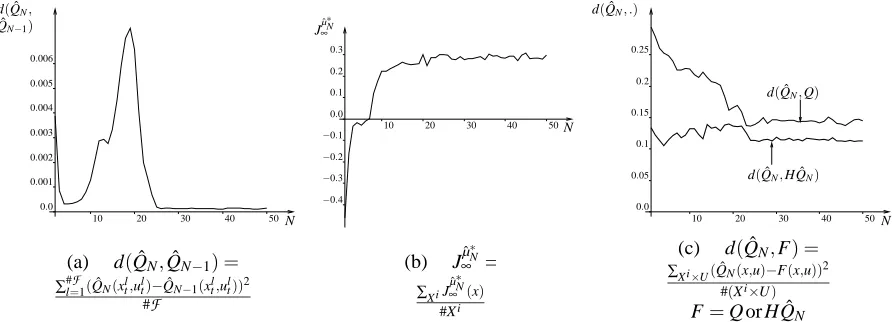
learning method. Elements of the sequence of functions ˆQN obtained are represented on Figure 3.

While the first functions of the sequence differ a lot, they gain in similarities when N increases which is confirmed by computing the distance on

F

We observe that the distance rapidly decreases but, due to the fact that the tree structure is refreshed at each iteration, never vanishes.

100.

75.

50.

25.

0.0

0.0 2.5 5. 7.5 10._x

ˆ

Q1(x,−2)

ˆ

Q1(x,2)

ˆ Q1 100. 75. 50. 25.

0.0

0.0 2.5 5. 7.5 10. _x

ˆ

Q2

ˆ

Q2(x,−2)

ˆ

Q2(x,2)

0.0 2.5 5. 7.5 10._x

ˆ

Q3

ˆ

Q3(x,−2)

ˆ

Q3(x,2)

100.

75.

50.

25.

0.0

0.0 2.5 5. 7.5 10._x

100.

75.

50.

25.

0.0

ˆ

Q4(x,−2)

ˆ

Q4(x,2)

ˆ

Q4

0.0 2.5 5. 7.5 10. _x

100.

75.

50.

25.

0.0

ˆ

Q5

ˆ

Q5(x,2)

ˆ

Q5(x,−2)

0.0 2.5 5. 7.5 10._x

100.

75.

50.

25.

0.0

ˆ

Q10

ˆ

Q10(x,−2)

ˆ

Q10(x,2)

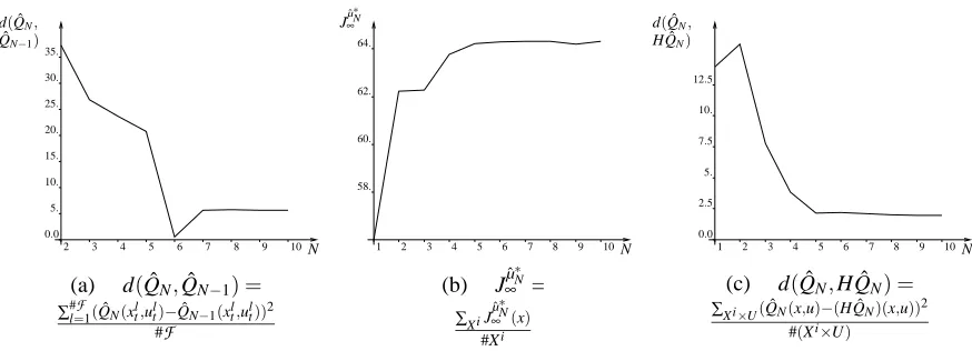
Figure 3: Representation of ˆQN for different values of N. The setF is composed of 2010 elements and the supervised learning method used is Pruned CART Tree.

2 3 4 5 6 7 8 9 10 35. 30. 25. 20. 15. 10. 5.

0.0

N d(_Qˆ_N,

ˆ

QN−1)

1 2 3 4 5 6 7 8 9 10_N 58.

60.

62.

64.

J_∞ˆµ∗N

1 2 3 4 5 6 7 8 9 10 0.0

2.5 5.

7.5 10.

12.5

N d(_Qˆ_N,

H ˆQN)

(a) d(_Qˆ_N,Qˆ_N −1) = ∑#F

l=1(QˆN(xtl,ult)−QˆN−1(xlt,ult))2 #F

(b) Jˆµ∗N ∞ = ∑_{X i}Jˆµ

∗ N ∞ (x) #Xi

(c) d(_Qˆ_{N,H ˆQN) =} ∑X i×U(QˆN(x,u)−(H ˆQN)(x,u))2

#(Xi_×U)

From the function ˆQNwe can determine the policy ˆµN. States x for which ˆQN(x,2)≥QˆN(x,−2)

correspond to a value of ˆµN(x) =2 while ˆµN(x) =−2 if ˆQN(x,2)<QˆN(x,−2). For example, ˆµ∗₁₀

consists of choosing u=₋2 on the interval[0,2.7[and u=2 on[2.7,10]. To associate a score to each policy ˆµ∗_N, we define a set of states Xi=_{0,1,2,···,10}, evaluate JˆµN

∞ (x)for each element of

this set and average the values obtained. The evolution of the score of ˆµ∗_N with N is drawn on Figure 4b. We observe that the score first increases rapidly to become finally almost constant for values of

N greater than 5.

In order to assess the quality of the functions ˆQN computed, we have computed the Bellman

residual of these ˆQN-functions. We observe in Figure 4c that even if the Bellman residual tends to

decrease when N increases, it does not vanish even for large values of N. By observing Table 2, one can however see that by using 6251 four-tuples (1000 episodes) rather than 2010 (300 episodes), the Bellman residual further decreases.

5.2.3 INFLUENCE OF THETREE-BASEDMETHOD

When dealing with such a system for which the dynamics is highly stochastic, pruning is necessary, even for tree-based methods producing an ensemble of regression trees. Figure 5 thus represents the

ˆ

QN-functions for different values of N with the pruned version of the Extra-Trees. By comparing

this figure with Figure 3, we observe that the averaging of several trees produces smoother functions than single regression trees.

By way of illustration, we have also used the Extra-Trees algorithm with fully developed trees (i.e., nmin=2) and computed the ˆQ10-function with the fitted Q iteration using the same set of

four-tuples as in the previous section. This function is represented in Figure 6. As fully grown trees are able to match perfectly the output in the training set, they also catch the noise and this explains the chaotic nature of the resulting approximation.

Table 2 gathers the Bellman residuals of ˆQ10obtained when using different tree-based methods

and this for different sets of four-tuples. Tree-based ensemble methods produce smaller Bellman residuals and among these methods, Extra-Trees behaves the best. We can also observe that for any of the tree-based methods used, the Bellman residual decreases with the size of

F

Note that here, the policies produced by the different tree-based algorithms offer quite similar

scores. For example, the score is 64.30 when Pruned CART Tree is applied to the 2010 four-tuple

set and it does not differ from more than one percent with any of the other methods. We will see that the main reason behind this, is the simplicity of the optimal control problem considered and the small dimensionality of the state space.

5.2.4 FITTEDQ ITERATION ANDBASISFUNCTIONMETHODS

We now assess performances of the fitted Q iteration algorithm when combined with basis function methods. Basis function methods suppose a relation of the type

o=

nbBasis

∑

j=1

cjφj(i) (23)

between the input and the output where cj ∈Rand where the basis functionsφj(i)are defined on

architec-100.

75.

50.

25.

0.0

0.0 2.5 5. 7.5 10._x

ˆ

Q1

ˆ

Q1(x,−2)

ˆ

Q1(x,2)

100.

75.

50.

25.

0.0

0.0 2.5 5. 7.5 10._x

ˆ

Q2

ˆ

Q2(x,2)

ˆ

Q2(x,−2)

0.0 2.5 5. 7.5 10._x

ˆ Q3 100. 75. 50. 25.

0.0

ˆ

Q3(x,−2)

ˆ

Q3(x,2)

0.0 2.5 5. 7.5 10._x

100.

75.

50.

25.

0.0

ˆ

Q4

ˆ

Q4(x,2)

ˆ

Q4(x,−2)

0.0 2.5 5. 7.5 10._x

100.

75.

50.

25.

0.0

ˆ

Q5

ˆ

Q5(x,−2)

ˆ

Q5(x,2)

0.0 2.5 5. 7.5 10._x

100.

75.

50.

25.

0.0

ˆ

Q10

ˆ

Q10(x,−2)

ˆ

Q10(x,2)

Figure 5: Representation of ˆQN for different values of N. The setF is composed of 2010 elements and the supervised learning method used is the Pruned Extra-Trees.

0.0 2.5 5. 7.5 10._x

100.

75.

50.

25.

0.0

ˆ

Q10

ˆ

Q10(x,−2)

ˆ

Q10(x,2)

Figure 6: Representation of ˆQ10 when Extra-Trees is used with no pruning

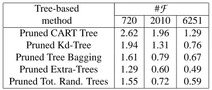
Tree-based method

#F

720 2010 6251 Pruned CART Tree 2.62 1.96 1.29 Pruned Kd-Tree 1.94 1.31 0.76 Pruned Tree Bagging 1.61 0.79 0.67 Pruned Extra-Trees 1.29 0.60 0.49 Pruned Tot. Rand. Trees 1.55 0.72 0.59

Table 2: Bellman residual of ˆQ10. Three different sets of four-tuples are used. These sets have been generated by considering 100, 300 and 1000 episodes and are composed respectively of 720, 2010 and 6251 four-tuples.

ture. The training set is used to determine the values of the different cj by solving the following

minimization problem:13

13. This minimization problem can be solved by building the(#TS×nbBasis)Y matrix with Yl j=φj(il). If YTY

is invertible, then the minimization problem has a unique solution c= (c1,c2,···,cnbBasis)given by the following

expression: c= (YTY)−1_YT_{b with b∈R}#TS_{such that b}

l=ol. In order to overcome the possible problem of

non-invertibility of YTY that occurs when solution of (24) is not unique, we have added to YTY the strictly definite positive matrixδI, whereδis a small positive constant, before inverting it. The value of c used in our experiments as solution of (24) is therefore equal to(YTY+δI)−1_YT_{b whereδhas been chosen equal to 0}

Extra-Trees

0.0 0.5 1.

1.5 2.

2.5

Grid size

d(Qˆ10, H ˆQ10)

10 20 30 40

piecewise-linear grid piecewise-constant grid

0.0 2.5 5. 7.5 10.

0.0 25. 50. 75. 100. ˆ Q10 x ˆ

Q10(x,2)

ˆ

Q10(x,−2)

0.0 2.5 5. 7.5 10.

0.0 25. 50. 75. 100. ˆ Q10 x ˆ

Q10(x,2)

ˆ

Q10(x,−2)

(a) Bellman residual of ˆQ10

(b) ˆQ10computed when using a 28 piecewise-constant grid as approx. arch.

(c) ˆQ10computed when using a 7 piecewise-linear

grid as approx. arch.

Figure 7: Fitted Q iteration with basis function methods. Two different types of approximation architectures are considered: piecewise-constant and piecewise-linear grids. 300 episodes are used to generate

F.

arg min (c1,c2,_···,cnbBasis)∈RnbBasis

#TS

∑

∑

cjφj(il)−ol)2. (24)

We consider two different sets of basis functionsφj. The first set is defined by partitioning the

state space into a grid and by considering one basis function for each grid cell, equal to the indicator function of this cell. This leads to piecewise constant ˆQ-functions. The other type is defined by

partitioning the state space into a grid, triangulating every element of the grid and considering that ˆ

Q(x,u) =∑v_{∈Vertices(x)}W(x,v)Qˆ(v,u)where Vertices(x)is the set of vertices of the hypertriangle x belongs to and W(x,v)is the barycentric coordinate of x that corresponds to v. This leads to a set of overlapping piecewise linear basis functions, and yields a piecewise linear and continuous model. In this paper, these approximation architectures are respectively referred to as piecewise-constant

grid and piecewise-linear grid. The reader can refer to Ernst (2003) for more information.

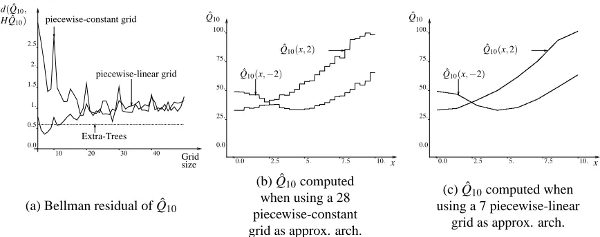
To assess performances of fitted Q iteration combined with constant and piecewise-linear grids as approximation architectures, we have used several grid resolutions to partition the interval[0,10](a 5 grid, a 6 grid, ···, a 50 grid). For each grid, we have used fitted Q iteration

with each of the two types of approximation architectures and computed ˆQ10. The Bellman

resid-uals obtained by the different ˆQ10-functions are represented on Figure 7a. We can see that basis

function methods with piecewise-constant grids perform systematically worse than Extra-Trees, the tree-based method that produces the lowest Bellman residual. This type of approximation archi-tecture leads to the lowest Bellman residual for a 28 grid and the corresponding ˆQ10-function is

sketched in Figure 7b. Basis function methods with piecewise-linear grids reach their lowest Bell-man residual for a 7 grid, BellBell-man residual that is smaller than the one obtained by Extra-Trees. The corresponding smoother ˆQ10-function is drawn on Figure 7b.

state space dimensionality increases, piecewise-constant or piecewise-linear grids do not compete anymore with tree-based methods. Furthermore, we will also observe that piecewise-linear grids may lead to divergence to infinity of the fitted Q iteration algorithm (see Section 5.3.3).

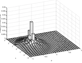
5.3 The “Car on the Hill” Control Problem

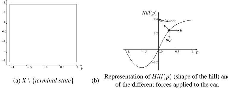
We consider here the “Car on the Hill” optimal control problem whose precise definition is given in Appendix C.2.

A car modeled by a point mass is traveling on a hill (the shape of which is given by the func-tion Hill(p) of Figure 8b). The action u acts directly on the acceleration of the car (Eqn (31),

Appendix C) and can only assume two extreme values (full acceleration (u=4) or full deceleration

(u=₋4)). The control problem objective is roughly to bring the car in a minimum time to the top

of the hill (p=1 in Figure 8b) while preventing the position p of the car to become smaller than

−1 and its speed s to go outside the interval[₋3,3]. This problem has a (continuous) state space of dimension two (the position p and the speed s of the car) represented on Figure 8a.

Note that by exploiting the particular structure of the system dynamics and the reward function of this optimal control problem, it is possible to determine with a reasonable amount of computation the exact value of J_∞µ∗ (Q) for any state x (state-action pair(x,u)).14

3.

2.

1.

0.0

−1.

−2.

−3.

−1. −.5 0.0 0.5 1.

s

p

p u

−0.2 0.2 0.4

−1. ₋.5 0.0 0.5 1.

Resistance

mg Hill(p)

(a) X_{\ {}terminal state_} (b) Representation of Hill(p)(shape of the hill) and

of the different forces applied to the car.

Figure 8: The “Car on the Hill” control problem.

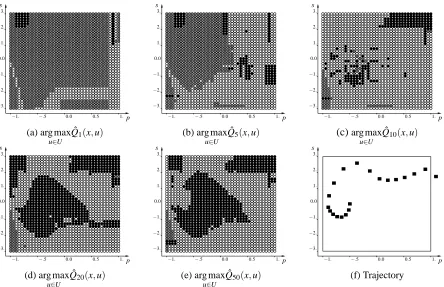
5.3.1 SOMEBASICRESULTS

To generate the four-tuples we consider episodes starting from the same initial state corresponding to the car stopped at the bottom of the hill (i.e.,(p,s) = (−0.5,0)) and stopping when the car leaves the region represented on Figure 8a (i.e., when a terminal state is reached). In each episode, the action ut at each time step is chosen with equal probability among its two possible values u=−4

and u=4. We consider 1000 episodes. The corresponding set

F

Note that during these 1000 episodes the reward r(xt,ut,wt) =1 (corresponding to an arrival of the

car at the top of the hill with a speed comprised in[₋3,3]) has been observed only 18 times.

3.

2.

1.

0.0

−1.

−2.

−3.

−1. ₋.5 0.0 0.5 1.

s

p

3.

2.

1.

0.0

−1.

−2.

−3.

−1. ₋.5 0.0 0.5 1.

s

p

3.

2.

1.

0.0

−1.

−2.

−3.

−1. ₋.5 0.0 0.5 1.

s

p

(a) arg max u∈U

ˆ

Q1(x,u) (b) arg max u∈U

ˆ

Q5(x,u) (c)arg max u∈U

ˆ Q10(x,u) 3.

2.

1.

0.0

−1.

−2.

−3.

−1. −.5 0.0 0.5 1.

s

p

3.

2.

1.

0.0

−1.

−2.

−3.

−1. −.5 0.0 0.5 1.

s

p

3.

2.

1.

0.0

−1.

−2.

−3.

−1. −.5 0.0 0.5 1.

s

p

(d) arg max u∈U

ˆ

Q20(x,u) (e) arg max u∈U

ˆ

Q50(x,u) (f) Trajectory