Speedup Learning for Repair-based Search by Identifying Redundant Steps

(1)

Speedup Learning for Repair-based Search

by Identifying Redundant Steps

Computer Science Department Technion, Haifa 32000, Israel

Editor: Thomas G. Dietterich

Abstract

Repair-based search algorithms start with an initial solution and attempt to improve it by iter-atively applying repair operators. Such algorithms can often handle large-scale problems that may be difficult for systematic search algorithms. Nevertheless, the computational cost of solving such problems is still very high. We observed that many of the repair steps applied by such algorithms are redundant in the sense that they do not eventually contribute to finding a solution. Such redun-dant steps are particularly harmful in repair-based search, where each step carries high cost due to the very high branching factor typically associated with it.

Accurately identifying and avoiding such redundant steps would result in faster local search without harming the algorithm’s problem-solving ability. In this paper we propose a speedup learn-ing methodology for attainlearn-ing this goal. It consists of the followlearn-ing steps: definlearn-ing the concept of a redundant step; acquiring this concept during off-line learning by analyzing solution paths for training problems, tagging all the steps along the paths according to the redundancy definition and using an induction algorithm to infer a classifier based on the tagged examples; and using the acquired classifier to filter out redundant steps while solving unseen problems.

Our algorithm was empirically tested on instances of real-world employee timetabling prob-lems (ETP). The problem solver to be improved is based on one of the best methods for solving some large ETP instances. Our results show a significant improvement in speed for test problems that are similar to the given example problems.

1. Introduction

One of the most important techniques developed in the field of Artificial Intelligence is problem solving by searching in state spaces. For some problems, the goal of the solver is to find a path from an initial state to a final state. Many search algorithms have been devised to find a low-cost or lowest-cost solution path.

(2)

A

B

C

D

E

F

G

H

I

J

K

L

0.5

0.5 1

1 1

1

1 1

1 1 1 1

1

1 1 1 1 1 1

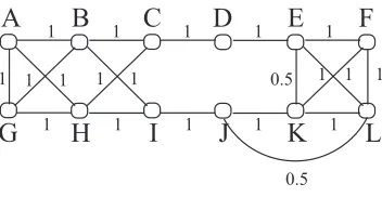
Figure 1: A TSP instance.

Examples for such methods are hill climbing, simulated annealing (Kirpatrick et al., 1983) and tabu search (Glover, 1989).

Local search algorithms can often handle large-scale problems that may be difficult for system-atic search algorithms (Minton et al., 1992). Nevertheless, the computational cost of solving such problems is still very high. We observed that many of the repair steps applied by such algorithms are redundant in the sense that they do not eventually contribute to finding a solution. Such redundant steps are particularly harmful in repair-based search, where each step carries high cost due to the very high branching factor typically associated with it.

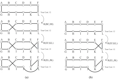
Assume, for example, that we try to solve an instance of the Traveling Salesperson Problem (TSP) by iterative repair. We start with a suboptimal tour and iteratively repair it by removing two of its edges and replacing them with the two edges that complete it into a legal tour of lower cost (Lin and Kernighan, 1973). To avoid local minima we allow also replacements that do not change the tour cost. Figure 1 shows a TSP instance. Figure 2(a) shows a sequence of steps leading to a solution generated by the above algorithm. The first step is redundant since removing it would have still resulted in a solution as demonstrated in Figure 2(b).

Accurately identifying and avoiding such redundant steps would result in faster local search without harming the algorithm’s problem-solving ability. In this paper we propose a speedup learn-ing methodology for attainlearn-ing this goal. Our methodology is based on the followlearn-ing steps:

1. Defining the concept of a redundant step.

2. Acquiring this concept during off-line learning by analyzing solution paths for training prob-lems, tagging all steps along the paths according to the redundancy definition, and using an induction algorithm to infer a classifier based on the tagged examples.

3. Using the acquired classifier to filter out redundant steps while solving unseen problems.

(3)

A B C D E F

G H I J K L

A B C D E F

G H I J K L

A B C D E F

G H I J K L

A B C D E F

G H I J K L

Tour Cost: 12

Tour Cost: 11 Tour Cost: 12

R(BC,HI)

R(EF,KL)

R(EL,JK)

A B C D E F

G H I J K L

A B C D E F

G H I J K L

A B C D E F

G H I J K L

Tour Cost: 12

Tour Cost: 11 Tour Cost: 12

R(EF,KL)

R(EL,JK)

(a) (b)

Figure 2: Applying iterative repair to a TSP instance. Figure (a) shows the sequence leading to an optimal tour. Figure (b) shows the results of applying the sequence without the first redundant operator.

4 describes the empirical evaluation of the algorithm on two real ETPs. Finally, in Section 5, we compare our approach to alternative speedup learning approaches and present our conclusions.

2. Speedup Learning for Repair Based Methods by Identifying Redundant Search Steps

In this section we give some background about local search and describe our algorithms for utilizing and learning the redundancy concept.

2.1 Local Search Algorithms

We start with a formal description of the local search approach. Let S be a set of states. Let s0be a start state. Let G⊆S be a set of goal states. Let O be a finite set of operators. An operator o∈O is a function from Dom(o)(Dom(o)⊆S) to S. If s6∈Dom(o), we define o(s)to be s. Letσ=o1,...,on

be a sequence of operators in O. We defineσ(s) =on(...o1(s)).

(4)

procedure LocalSearch(s0,GOAL,O) s←s0

Repeat until GOAL(s)do begin

Os← {o∈O|s∈Dom(o)};legal operators in s

o←Select(Os,s)

s←o(s) end

return s

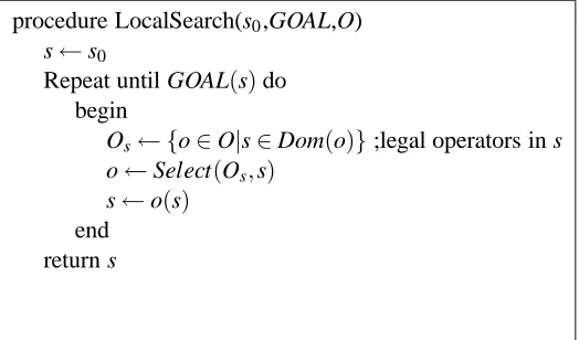
Figure 3:A general scheme for local search.

We assume that a predicate GOAL that tests for membership in G is given. The formal description of the algorithm is given in Figure 3.

Many of the local search methods can be characterized by their select procedure. Steepest-descent hill climbing selects the operator that yields the best state with respect to a given heuristic function. Simple hill climbing selects the first operator that improves the current state. Hill-climbing methods are known to be sensitive to local minima and plateaus. Simulated annealing (Kirpatrick et al., 1983) attempts to overcome these problems by allowing selecting non-improving operators. Tabu search (Glover, 1989) avoids utilizing the last k operators used.

2.2 Local Search Using a Redundancy Filter

Local search algorithms repeatedly modify the current state in order to reach a goal state. Some of these local changes may be redundant in the sense that they do not contribute to reaching a goal state. More formally, we define a step ho,sito be redundant with respect to a goal G iff for any sequenceσof operators(o||σ)(s)∈G⇒σ(s)∈G (||stands for the concatenation operator).

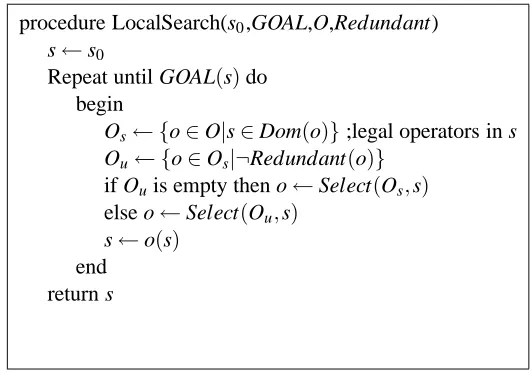
If we could identify redundant steps, we could speed up our local search by avoiding them. Figure 4 shows the local search scheme with the redundancy test incorporated. The algorithm first finds the set of operators that are legal at the current state. It then uses the redundancy predicate to filter out of this set operators that are estimated to be redundant. The select procedure is then applied to the reduced set. If the redundancy predicate is computationally expensive, we can switch the order of filtering. First the algorithm selects a window of best (or almost best) operators according to its select procedure. Then it chooses the first nonredundant operator out of this set. An example for an algorithm that uses this order of filtering is given in Section 3.

2.3 Learning the Redundancy Concept

(5)

procedure LocalSearch(s0,GOAL,O,Redundant) s←s0

Ou← {o∈Os|¬Redundant(o)}

if Ouis empty then o←Select(Os,s)

else o←Select(Ou,s)

s←o(s) end

return s

Figure 4:A general scheme for local search that avoids redundant steps.

and are given to an inductive concept learner. The resulting classifer is then used as a redundancy estimator as described in Figure 4.

The algorithm in Figure 4 tests each of the legal steps for redundancy. In practice, however, we are only interested in detecting those redundant steps that might be considered useful by the prob-lem solver. Such potentially useful steps will be selected by the select procedure. Steps which are selected by the select procedure but turn out to be redundant are called deceptively redundant. Dur-ing the learnDur-ing process, we concentrate on deceptively redundant steps by restrictDur-ing our example set to steps along solution paths.

To estimate the redundancy of applying an operator o to a state s in a problem p=hs0,G,Oi, the algorithm tests whether skipping this application would have also resulted in a goal state.1 More formally, let σ=o0,...,oi,...,on be a sequence of operators applied by the given local search

algorithm to reach a solution state. Thus,σ(s0)∈G. Let si =o0,...,oi−1(s0). We taghsi,oi,pias

redundant iff oi+1,...,on(si)∈G.

Note that this tagging procedure only approximates our defined concept of redundancy. We do not test whether every solution sequence from oi(si)is also a solution sequence from si but are

rather satisfied with testing one such case. This is not as harmful as it seems since the particular solution tested is the one generated by the specific problem solver that the learner tries to improve. Moreover, it is necessary in complex domains where testing all possible solution sequences from a given state is impractical. Alternatively, we could use a limited sample of solution sequences to improve the redundancy approximation (but increase the learning cost).

The next step is to convert each tagged step to a feature vector representation. This step requires domain-specific features to be supplied by the user. In search spaces with a standard predefined structure, such as CSP spaces, it is possible to define general features. Such features will be based on the particular representation of states and operators. In Section 3.3 we will show a set of features for ETPs.

(6)

As soon as we have a set of tagged feature vectors, we can use any of the known induction algorithms to learn the redundancy concept. Since the goal of the learning process is to speed up a problem solver, we must use a fast classifier. For example, in the experiments described in Section 4.1, we use a decision tree as our classifier. Furthermore, during classification we compute the features on demand to reduce the overall classification cost of the decision tree.

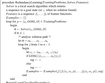
procedure RedundancyLearning(TrainingProblems,Solver,Features) Solver is a local search algorithm which returns

a sequence to a goal state (or⊥when no solution found). Features is a sequence f1,...,fkof feature functions.

Examples←{}

loop for p=hso,GOAL,Oi ∈TrainingProblems

begin

σ←Solver(so,GOAL,O)

ifσ6=⊥

/* analyze solution path */

letσ=o0,...,oi,...,on

loop for j from 1 to n−1 begin

let sj=ho0,...,oj−1i(s0) if GOAL(hoj+1,...,oni(sj))

tag←+ else

tag← −

Examples←ExamplesShhf1(sj,oj,p),...,fk(sj,oj,p)i,tagi

end end

Return(LearnClassifier(Examples))

Figure 5:The learning algorithm.

The learning algorithm is described formally in Figure 5. The algorithm assumes that the given features are functions whose domain is a step and a problem.

2.4 Generating Training Problems

The goal of a speedup learning system is to improve the potential performance of the problem solver on future problems. Most learning paradigms, such as the PAC framework (Valiant, 1984), assume that the past problems and the future problems are drawn from the same fixed distribution. This implies that the past examples are considered as a set, and the order of their appearance is ignored.

(7)

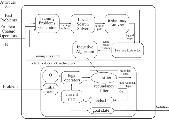
Inductive Algorithm Past Problems Local Search Solver initial state Solution Learning algorithm adaptive-Local-Search-solver Redundancy Analyzer Feature Extractor Attribute Set training problem Problem-Change Operators B Training Problems

Generator solutionpath

tagged steps tagged feature vectors Problem current state O s legal operators Os redundancy filter Ou Select o classifier redundant steps non-redundant steps goal state

Figure 6: System description scheme.

In off-line learning, an automatic generation of training problems is often required. A reasonable approach to this task is to try and generate problems that are likely to resemble future problems. For the PAC-like problem model, it is reasonable to generate problems that are similar to the set of past problems regardless of their order. For the DCSP model described above, the next problem will most resemble the last problem. Therefore, this problem can be used as the basis for training problem generation. Assume that a set of atomic problem-change operators is given. In DCSP, for example, such operators can be implemented by the removal or addition of constraints. We define the distance d between two problems p1and p2as the minimal number of problem-change operators required to transform p1 into p2. We assume that at any time t, a bound B on the distance between the last problem pt and the next problem pt+1is either given or can be estimated from the sequence of externally supplied past problems hp1,...,pti. For example, if we assume that the distance is

distributed uniformly over the sequence, we can assume that

max

i=1,...,t−1{d(pi,pi+1)} ≈i=max1,...,t{d(pi,pi+1)}.

Training problems can then be generated by applying to the last problem a random sequence of change operators, with length bounded by the above bound.

2.5 A General Architecture for Learning and Using a Redundancy Filter

(8)

3. Applying Redundancy-based Speedup Learning to ETPs

In this work we are particularly interested in speeding up the solution of ETPs. We start with a description of ETPs and continue with local search techniques used to solve such problems. We then show how to apply our algorithm to speed up these search techniques. For this we describe a set of features appropriate for ETP learning.

3.1 The Employee Timetabling Problem

Many organizations face the problem of employee timetabling, where a set of employees needs to be assigned a set of tasks in a set of fixed time shifts. The problem is typically specified by listing the set of employees with their qualifications, constraints and preferences, and the set of tasks to be fulfilled in each shift. In addition, there is commonly a set of constraints enforced by the organization. Such problems include assignment of nurses to shifts in a hospital or assignment of production workers to shifts in a factory. Related and very similar problems are school timetabling (Junginger, 1986), and examination timetabling (Carter, 1986). Schaerf (1995) gives a survey of research in this area.

We start with an exact definition of ETP, largely based on the work of Schaerf and Meisels (1999). The Employee Timetabling Problem consists of assigning employees to tasks in shifts with fixed start and end times.

Definition 1 An employee timetabling domain is a triplethE,S,Tiwhere:

• E is a set of employees;

• S is a set of shifts;

• T is a set of tasks.

For example, in hospital timetabling, a shift can be “Tuesday morning” and a task can be “head nurse”. The set of shifts spans over a period (a week, for example).

Definition 2 A timetabling assignment is a functionϕ: E×S→T∪ {φ}.

ϕ(e,s) =t means that employee e is assigned to task t in shift s. If employee e is not assigned to any task in shift s thenϕ(e,s) =φ. In this case we say that e is assigned to the null task. Note that by the above definition an employee can be assigned to at most one task in a shift. For convenience we will represent an assignment as a two-dimensional matrix, M, where M[e,s] =t.

A timetabling constraint is a predicate over timetabling assignments. Schaerf and Meisels de-scribe five types of such constraints:

• A requirement constraint. An overrequirement constraint is a tripleths,t,rmaxi where s∈S

and t∈T . M satisfies such a constraint iff the number of employees assigned to task t in shift s is not more than rmax. An underrequirement constraint is a triplet hs,t,rmini. M satisfies

such a constraint iff the number of employees assigned to task t in shift s is at least rmin. For

example, there must be two to four regular nurses on the Sunday evening shift.

• An ability constraint. This is a pair he,Tei where e∈E and Te ⊆T . M satisfies such a

constraint iff employee e is only assigned to tasks from Te. For example, Jane can work as a

(9)

• An availability constraint. This is a pairhe,si where e∈E and s∈S. M violates such a constraint iff employee e is assigned to work in shift s. For example, John cannot work on Wednesday evening.

• A conflict constraint. This is a triplethe,s1,s2iwhere e∈E and s1,s2∈S. M violates such a constraint iff employee e is assigned to work in both shifts s1and s2. For example, the orga-nization may enforce a constraint where no employee is allowed to work in two consecutive shifts. In addition, Jane is able to work on either Saturday evening or Sunday evening but not in both shifts.

• A workload constraint. An overload constraint is a triplethe,Se,rmaxiwhere e∈E and Se⊆S.

M satisfies such a constraint iff the number of shifts in Se where e is assigned to work is no

more than rmax. For example, no worker is allowed to work more than two night shifts each

week. An underload constraint is a triplethe,Se,rminiwhere e∈E and Se ⊆S. M satisfies

such a constraint iff the number of shifts in Se where e is assigned to work is at least rmin.

A timetabling problem is a pair consisting of a domain and a set of constraints. Our goal is to find an assignment that satisfies all of the constraints. An alternative goal may be to find an assignment that optimizes some criterion such as minimizing the total wages paid to employees or equalizing the workload over the set of employees. Even et al. (1976) proved that these problems belong to the class of NP-complete problems. Despite the difficulty, many methods have been developed to cope with timetabling problems. Roughly speaking, there are two principal fields that deal with these problems: Operations Research (Burns and Carter, 1985; Nanda and Browner, 1992; Schaerf, 1995), and Artificial Intelligence (Duncan, 1990; Schaerf and Schaerf, 1995; Schaerf, 1995, 1996; Meisels et al., 1996; Meisels and Lusternik, 1997; Meisels et al., 2000, 1997; Banks et al., 1998; Schaerf and Meisels, 1999). The former includes linear programming, reduction to graph coloring, and network flow techniques. The latter includes genetic algorithms, local search, constraint satisfaction, and expert systems/rule-based approaches. In the next subsection we describe the local search technique proposed by Schaerf and Meisels. The problem solver our learning algorithm attempts to improve is based on this technique.

3.2 Local Search for ETPs

There are quite a few local search algorithms that were applied to ETPs (Schaerf and Schaerf, 1995; Schaerf, 1996; Schaerf and Meisels, 1999; Meisels and Schaerf, 2003). The problem solver targeted by our speedup learning algorithm is based on the techniques developed by Schaerf and Meisels (1999) and applied successfully to real-life ETPs.

Since the problem-solving technique is based on the local search algorithm described in Figure 3, we need only to specify the following components: the set of search states, the set of operators, the GOAL predicate, and the decision procedure select which chooses the next operator to apply. The rest of this section describes these components.

(10)

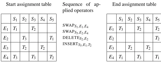
Start assignment table Sequence of ap-plied operators

End assignment table

S1 S2 S3 S4 S5

E1 T1 T2

E2 T3 T1

E3 T2 T2

E4 T3 T3 T2

SWAPS1,E1,E4

SWAPS5,E2,E4

DELETES2,E2

INSERTS5,E1,T2

S1 S2 S3 S4 S5

E1 T3 T2 T2

E2 T2

E3 T2 T2

E4 T1 T3 T1

Figure 7:The effect of applying a sequence of operators to an assignment table.

1. Swap.2 This operator is instantiated by three parameters: shift s, employee e1, and employee e2. The instantiated operator swaps the tasks of e1 and e2 in shift s. We denote such an operator bySWAPs,e1,e2.

2. Insert. This operator is instantiated by three parameters: shift s, employee e, and a non-null task t. The instantiated operator assigns task t to employee e in shift s. It is not legal to apply the operator if e is already assigned a non-null task in shift s. We denote such an operator by INSERTs,e,t.

3. Delete. This operator is instantiated by two parameters: shift s and employee e. The instanti-ated operator assigns the null task to employee e in shift s. It is not legal to apply the operator if e is already assigned the null task in shift s. We denote such an operator byDELETEs,e.

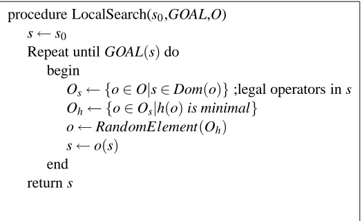
Figure 7 shows the results of applying a sequence of operators on an example state (timetabling assignment). Our goal is to search for a state without any violated constraints. Thus, the goal predicate checks whether the total number of violated constraints is zero. At each iteration, the select operator must choose one operator from the set of legal operators for the current state. Our strategy first randomly selects one of the three operator types. It then applies a heuristic function on the states resulting from applying all3 operators of the selected type and selects the one with best heuristic value. The heuristic used is the minimum-conflict function (Minton et al., 1992), which counts the number of violated constraints. Schaerf and Meisels used a more complicated heuristic that also includes some look-ahead component and a shifting penalty scheme to dynamically determine the weight of each constraint type. We preferred the simpler heuristic because it proved to be faster on the tested domains and therefore a more challenging choice for speedup learning. Frequently, this heuristic results in a relatively large set of best operators. In such cases we use random tie-breaking. We refer to the algorithm described in this subsection as the GSHC* scheduler. The algorithm is formally described in Figure 8.

2. The original name given by Schaerf and Meisels is Replace. A swap operator is not the same as replace, but a simple extension of it.

(11)

procedure LocalSearch(s0,GOAL,O) s←s0

Oh← {o∈Os|h(o)is minimal}

o←RandomElement(Oh)

s←o(s) end

return s

Figure 8:TheGSHC* scheduler algorithm.

3.3 Features for ETP Domains

In the previous section we described the redundancy-learning algorithm that induces a classifier based on tagged examples. For ETP, each example is a triplethM,o,piwhere M is an assignment table representing a state, o is an operator, and p is an ETP instance. In order to generalize from a training problem to future unseen problems, we convert the examples to feature vector representa-tion. The features are usually domain-dependent. In this subsection we describe a set of features for the ETP domain. These features have been selected out of a larger group by experimenting4 on test sets.

The features can be divided to two groups: atomic features and compound features. The atomic features can be categorized according to the parts of the example they pertain to:

• State-problem attributes. These are defined over a state M. They try to capture its charac-teristics with respect to the problem definition p. Each of the attributes of this group sums, for one constraint type, the values of its violations. For example, the maximum-employee violations attribute computes, for each violation of the overrequirement constraint, the differ-ence between the number of employees assigned to the given task in the given shift and the maximum allowed. It then sums these differences.

A high value for this feature may indicate that swap or insert operators are redundant since they do not reduce the number of such violations.

• Operator-state-problem attributes. While attributes of the previous group consider the whole assignment table M, attributes in this group consider only the part of the table defined by the instantiation of the variables of operator o. Thus, such features focus on the part of the state that may be more relevant to the specific operator considered.

For example, assume that the operator o is INSERTs,e,t. The operator-maximum-employee

violations attribute sums the number of redundant employees, according to overrequirement constraints in p, who are scheduled to perform task t in shift s.

(12)

A positive value for this attribute may indicate that the specific insertion is redundant since there are already enough employees in the given shift assigned to perform the given task. Note that it is quite possible that the specific insert operator is not redundant despite a positive value for this attribute. For example, it is possible that the particular employee is underloaded and the insertion allows an overloaded employee to be freed from this shift.

• State-operator attributes. These attributes are defined over the state M and the operator o. These attributes attempt to characterize the relations between the state and the operator re-gardless of the particular problem p. For example, assume that the operator o isDELETEs,e.

The employee workload attribute counts the number of shifts in which employee e is sched-uled to work. A low value may indicate that the employee has a low workload and that the operator may be redundant.

• Operator-problem attributes. These attributes are defined over the problem p and the operator o. These attributes attempt to characterize operator o with respect to problem p regardless of the particular state M. For example, assume that the operator o isINSERTs,e,t. The

employee-workload constraint degree attribute counts the number of employee-workload constraints in which employee e participates.

• Problem-base-problem attributes. These attributes try to characterize the problem itself. Since there are too many possible features for describing an ETP, we restrict ourselves to features that describe the differences between the problem and the base problem.

The class of compound attributes combines pairs of continuous atomic attributes by arithmetic relations of their values. An example is the attribute-i-bigger-than-attribute-k attribute, which tests whether the value of a specific attribute is bigger than the value of another specific attribute. The complete list of attributes can be found in Appendix A.

3.4 Problem-change Operators for Generating Training ETPs

For the ETP domains used in this paper, we made several reasonable assumptions that determine the set of problem-change operators. We assume that the only type of change is a replacement of an employee by a new one. This includes changes to certain constraints of an employee. We assume that the difference between the new employee and the replaced employee is restricted as follows:

1. The set of tasks Tnew defined by the ability constraints of the new employee is similar to that

of the replaced employee (Told). Specifically, we assume that either Told⊆Tnewor Tnew⊆Told

and

||Tnew| − |Told|| ≤εq|Told|.

This means that the new employee is either more qualified or less qualified than the replaced employee, but the difference in their qualifications is bounded. Thus, for example, such a restriction could be used to prevent replacing a nurse with an engineer.

2. The number of shifts for which the new employee is available,|Snew|, defined by the

availabil-ity constraints, is similar to the number of shifts for which the replaced employee is available,

|Sold|. Specifically, we assume that

(13)

procedure LocalSearch(s0,GOAL,O,redundant) s←s0

hmin←mino∈Osh(o)

Oh← {o∈Os|h(o)≤hmin(1+ε)}

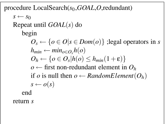
o←first non-redundant element in Oh

if o is null then o←RandomElement(Oh)

s←o(s) end

return s

Figure 9: The adaptive-GSHC* scheduler algorithm.

Such a restriction could be used, for example, to prevent replacing a full-time employee with a part-time employee.

We assume that the other two types of constraints, workload and conflict constraints, are based on organizational rules and are therefore not likely to be changed often. Of course, the framework presented here does not depend on these assumptions.

3.5 Utilizing the Learned Classifier for ETP

After the classifier is learned, it can be used for detecting redundant steps as described in the algo-rithm in Figure 4. In this algoalgo-rithm, we first filter the redundant operators out of the set of legal ones and then select the best operator. This approach is reasonable if the cost of applying the redun-dancy classifier is very low compared to the selection process. An application of a straightforward implementation of the minimum-conflict heuristic may carry a high computational cost in the ETP domain. Our implementation, however, follows an incremental approach, which yields a very ef-ficient heuristic computation. Since a heuristic evaluation is now much cheaper than a redundancy classification, we first find the best operators according to the heuristic and then return the first best operator that is not redundant. This version of the algorithm is described in Figure 9.

4. Experimental Evaluation

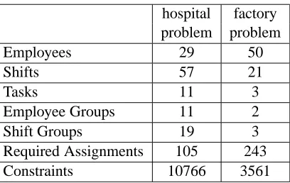
To test the effectiveness of our algorithm, we experimented with it in two real ETP domains. One, the hospital department problem, is timetabling of nurses in a hospital department. The other, the factory problem, is timetabling of production workers in a factory.5 In the hospital department problem, there are 57 shifts in each week’s timetable and 29 employees to be assigned to a total of 105 tasks over 7 days. The factory problem has 21 weekly shifts (three per day, 8 hours each)

(14)

hospital factory problem problem

Employees 29 50

Shifts 57 21

Tasks 11 3

Employee Groups 11 2

Shift Groups 19 3

Required Assignments 105 243

Constraints 10766 3561

Table 1:Quantitative information about the two problem instances used for experimentation.

and 50 employees to be assigned to a total of 243 tasks. Each of these problems includes several thousands of constraints. This data is summarized in Table 1. Each of the two instances is used as a base problem from which training and testing problems are generated. The exact specification of the two instances is listed in the online Appendix.

When representing the problems as a search space according to the scheme described in Section 3.2, the computed branching factor is about 42,000 for the hospital department problem and about 30,000 for the factory problem. The average actual branching factor (considering only nontrivial legal operators available in each search state) is 5000 for the hospital department problem and 6735 for the factory problem.

4.1 Experimental Methodology

Most of the experiments described here consist of a learning phase and a testing phase. We assume the model described in Section 2.4, where the learner is given the last problem, and a bound B on the distance between the last problem and the next problem.

For testing we use a set of 100 random problems with distance bounded by B from the input problem. We use the same set throughout our experiments. The problem solver we use for testing is theGSHC* scheduler described in Section 3.2. Since we assume that the next problem to be solved is similar to the last problem, it is reasonable to exploit the last solution for the new problem. One of the obvious ways of doing so is by using the last solution as an initial state for the next problem. We therefore use this modified scheduler with the same initial solution for all the tests.

For training, the learner gets as input the base problem, the bound B, a set of change operators and a set of features. The learner generates training problems using the algorithm described in Section 2.4. To reduce variability, we use the same training set for all the experiments. The learner generates from each solution path a set of tagged examples as described in Figure 5. The examples are given to the C4.5 induction algorithm (Quinlan, 1986, 1993), which generates a decision tree classifier. This classifier is then used by the adaptive-GSHC* scheduler algorithm for solving test problems.

(15)

(1994) that treats the results of such experiments as censored data. In particular, we used the most conservative approach. This approach considers as infinite the solving time of any problem in which the adaptive-GSHC* scheduler algorithm stopped due to a resource bound.

4.1.1 DEPENDENTVARIABLES

The goal of speedup learning is to improve the performance of the given problem solver. Therefore, the most important dependent variables are those measuring that improvement. In addition, to gain some insight about the learning process, we measure various aspects of the learned classifiers:

• Speedup factor. The ratio between the speed of the problem solver after learning (adaptive-GSHC* scheduler) and the speed before learning ((adaptive-GSHC* scheduler). The speed is measured by CPU time.6

• Atomic operator applications. The number of atomic operator applications, where swap is considered as either two or four atomic applications. This variable is independent of imple-mentation and can therefore be used by other researchers for comparison.

• Success rate. The portion of the test set that is solved by the tested algorithm.

• Accuracy on test examples. The average accuracy of the learned concept on the test set.

• Attribute class utility. The contribution of each class of attributes to the performance of the learning algorithm. This variable is measured by comparing performance with and without the tested set.

4.1.2 INDEPENDENT VARIABLES

There are many independent variables that affect the performance of the learning system. For the experiments described here we look at the following variables:

• Test distance variables. These variables determine the degree of difference between the base problem and the test problems. To generate a test problem, a sequence of problem change operators is applied to the base problem. Such a sequence is determined by the parameters listed below (see Subsection 2.4):

– Operator-distance variable. This is the length of the problem-change operator sequence (bounded by B, as mentioned in Subsection 2.4).

– Problem-change operator parameters. The problem-change operator for an ETP in-cludes two free parameters.

∗ εq. This parameter determines the degree of difference between the qualification

set of a replaced employee and that of the replacing employee. A smaller value indicates greater similarity between the two sets.

∗ εa. This parameter determines the degree of difference between the availability

set of a replaced employee and that of the replacing employee. A smaller value indicates greater similarity between the two sets.

(16)

scheduler Time Success Rate Atomic Operator

[Seconds] Applications

with without with without with without GRHC* scheduler 45 191 89 0 4150 18666 GRRSHC* scheduler 88 252 26 9 16976 39280 GRSSHC* scheduler 86 263 93 92 18633 50990 GSHC* scheduler 46 296 95 76 4260 28073

Table 2: Comparision of various search techniques when applied to the factory problem. The comparison is for time, success rate and atomic operator applications. The with columns give the performance of the appropriate scheduler when the solution to the base problem is used as the initial state. The

without columns give the performance of the appropriate scheduler that finds an initial state by

some greedy procedure.

The default values for these variables areεq=0.5 andεa=0.4. The operator distance is

uni-formly chosen from[1%,10%]. For example, for the factory problem this range is[1%,5%].

• Training distance variables. These variables determine the degree of difference between the base problem and the training problems. The default values for these variables areεq=0.5

and εa=0.4; and the operator distance is uniformly chosen from [1%,10%]. For example,

for the factory problem this range is[1%,5%].

• Learning resources. The most important independent variable for a learning system is the amount of resources invested in learning. The most common method of measuring learning resources in off-line learning is by counting the number of training problems. In our case this would not be a good measurement since there is a great variability in the difficulty of the training problems. Therefore we use instead the total number of tagged steps used in the classifier construction.

• Redundancy filter selectivity. This variable, which has the range [0,1], determines when a tree leaf should be tagged as nonredundant. If the portion of nonredundant examples in a leaf is above that value, the leaf is tagged as nonredundant; otherwise it is tagged as redundant. The default value of this variable is 0.5.

4.2 Performance Before Learning

To give our learning methodology a fair test, we were interested in a base algorithm that has both high success rate and high speed. The GSHC* scheduler algorithm selects from Os the set of all

legal operators. Schaerf and Meisels (1999) propose several methods for reducing the size of Os,

and therefore reducing the branching factor. We refer to the variants of the GSHC* scheduler that use these methods as follows:

• GRHC* scheduler. Select a random operator. Apply it if it improves the evaluation of the state.

(17)

hospital problem factory problem

Atomic operator applications 4500 4260

Success rate 70.0% 95.3%

Violations at end 0.59 0.05

Best operators per iteration 80 175

Solution length 2155 1774

Table 3: Comparing two test sets by applying to them theGSHC* scheduler. Each number represents the mean over the test sets.

• GRSSHC* scheduler. Select a random shift and a random employee. Select the best operator pertaining to the selected shift and employee.

Table 2 compares the performance of the four variants for the test set of the factory problem in terms of time,7success rate and atomic operator applications.

We can see that theGSHC* scheduler indeed has the best combination of speed and success rate. In addition, the table shows that it is beneficial to use a previous solution when the previous and current problems are similar. We therefore use this algorithm as our base algorithm to be improved. Table 3 shows the performance of theGSHC* scheduler on the two test sets. The table also reports the the total number of constraint violations for unsolved problems and the average number of best operators in each iteration (Ohin Figure 8).

4.3 Learning Curve

Our basic experiment tests the effect of the allocated learning resources on the utility of the adaptive-GSHC* scheduler. The learning algorithm generates solution paths for the training problems, ana-lyzes them and generates a set of tagged examples. These examples are used by the induction algorithm to build a classifier. We allocated enough learning resources to generate 150,000 exam-ples.

Before using the generated classifiers, we measured their accuracy on an independent set of tagged examples and found out that it is quite accurate: 89% on the hospital department problem and 76% on the factory problem. Accurate classification, however, is not sufficient for speedup. It is quite possible that the additional cost associated with the classifier applications will outweigh its benefits. The ultimate test should therefore be the speedup gained when using the learned classifier. We run the induction algorithm 5 times - with 0%,25%,50%,75% and 100% of the example set. Each time we compare the performance of the adaptive-GSHC* scheduler to that of the GSHC* scheduler. The learning curves showing the average speedup factor as a function of the learning resources for both domains are shown in Figure 10.

The graphs show typical learning curves with speedup factors of up to 1.5 and 3.1 for the hospital department problem and the factory problem respectively. According to the Wilcoxon test with the adjustment for censored data (as described in Subsection 4.1), the algorithm after learning (with 100% of the training data) significantly outperforms the algorithm before learning (with p=0.01).

(18)

0.5 1 1.5 2 2.5 3 3.5

0 20 40 60 80 100

Speedup Factor

Relative Size of Sample Set [%] Speedup Factor versus Learning Resources

hospital ETP factory ETP

Figure 10: The effect of learning resources on the speedup factor. Each number represents the mean over the test set.

GSHC* scheduler 70% 95%

adaptive-GSHC* scheduler 71% 99%

Table 4:The success rate before and after learning.

Of course, these results would have been less impressive had the increasing speed been accom-panied by reduction in the success rate of the problem solver. Table 4 shows that this is not the case. The success rate even increased slightly.

Table 5 shows the number of atomic operators before and after learning. We can see that for the factory problem, for example, the improvement measured by operator applications is a bit more than that represented by the speedup factor shown above (3.5 vs. 3.1). This difference is due to the overhead incurred by the classification process.

The third row of the table shows the results for the adaptive-GSHC* scheduler that, instead of using a learned classifier, uses an oracle that always gives the correct classification. (We use the same procedure utilized for tagging.) The number in this row can serve as a limit on the best possible improvement that can be achieved by our proposed algorithm.

(19)

GSHC* scheduler 4530 4260

adaptive-GSHC* scheduler 3020 1200

adaptive-GSHC* scheduler with oracle 1440 920

Table 5: The number of atomic operator applications before and after learning. The third row shows the results for the adaptive-GSHC* scheduler with oracle.

0.5 1 1.5 2 2.5 3 3.5

0.1 0.2 0.3 0.4 0.5 0.6 0.7 0.8 0.9

Speedup Factor

Classifier Threshold Speedup Factor versus Classifier Threshold

Figure 11:The effect of the filter selectivity on the speedup factor.

cost of classification, the effect of a false negative is more significant. We measured these errors and found that indeed for the factory problem the false negative error rate is smaller than for the hospital department problem– 11% versus 18%.

4.4 The Effect of the Filter Selectivity on Performance

At the end of a learning phase, the learned classifier is used to filter out steps that are estimated to be redundant. In this experiment we test the effect of the sensitivity of the filter on the system performance. Figure 11 shows the speedup factor as a function of the filter selectivity.

The graphs for the two problems show a similar behavior. A low value for the filter selectivity variable means a less selective filter. Such a filter will consider most of the steps as useful. Thus the likelihood of a redundant step passing through the filter and being selected is high. This is the reason for the lower performance with low values for the variable (values less than 0.5).

(20)

1000 2000 3000 4000 5000 6000 7000

0.1 0.2 0.3 0.4 0.5 0.6 0.7 0.8 0.9

Atomic Operator Applications

Classifier Threshold

Atomic Operator Applications versus Classifier Threshold

Figure 12:The effect of filter selectivity on atomic operator applications.

behavior of choosing a random step. High selectivity increases the likelihood of such incidents, which increases the chance of choosing a redundant step.

Figure 12 shows the number of atomic operator applications as a function of the filter selec-tivity. The graphs show patterns similar to those of the speedup factor. There is one interesting phenomenon in these graphs. Look at the graph for the factory problem at points 0.1 and 0.9. When the operator applications are compared, the performance for 0.9 is the same as for 0.1. However, when the same points on the speedup factor graph are compared, the performance for 0.9 is much worse.

A careful look at the algorithm (in Figure 9) will help explain this behavior. As the selectivity increases, so does the number of times that the classifier is applied. The overhead incurred by classification increases as well. Figure 13 shows the classifier overhead as a function of the filter selectivity. Indeed, while for the selectivity default value (0.5) the classification overhead is low (about 5%), for a value of 0.9 it increases to above 17%. The reason for the difference in overhead for the factory problem and the hospital department problem is that the percentage of redundant steps differs for each problem. Looking at Table 5 one can calculate the percentage of operators that are not redundant: 22% for the factory problem and 32% for the hospital department problem. Therefore, for the factory problem, the filter is applied more times before a nonredundant operator is found.

4.5 The Effect of the Problem Spread on the Learning Utility

(21)

0 2 4 6 8 10 12 14 16 18

0.1 0.2 0.3 0.4 0.5 0.6 0.7 0.8 0.9

Classifications Overhead [%]

Classifier Threshold

Classifications Overhead versus Classifier Threshold

Figure 13: The effect of filter selectivity on the classifications overhead. This overhead is given by the portion of total time that is consumed by the classifications.

B hospital problem factory problem

3% 1.4 2.2

10% 1.5 3.1

15% 1.2 2.55

Table 6:The effect of B on the speedup factor.

used throughout the experiments is 10%. Note that the actual distance between training and testing problems can be up to 2B, since both types of problems are sampled from a circle of radius B around the base problem.

To test the effect of B on the performance of the learning system, we repeated our learning experiment with B=3% and B=15%. The results are presented in Table 6 and Table 7 .

For B=15%, the benefit of learning decreases as expected since the testing problems are less similar to the training problems. For B=3% we anticipated that the performance would be bet-ter since the training and testing problems are more similar. The results, however, show that the speedup factor was no better. To understand the reason for this phenomenon, recall that the problem solver starts with the solution of the base problem as its initial state. Therefore, the solver will be able to efficiently solve problems that are very similar to the base problem even without learning. Consequently, the learning process has a narrower margin for improvement.

Other parameters that affect the difference areεqandεa, which determine the similarity between

(22)

B=3% B=10% B=15% GSHC* scheduler 94.5% 95.3% 95.3% adaptive-GSHC* scheduler 97.8% 99.5% 98.1%

Table 7:The effect of B on the success rate. The base problem is the factory problem.

attribute class Speedup Relative factor contribution problem-base-problem 2.71 14%

state-problem 1.47 110%

operator-state-problem 1.90 63%

state-operator 2.06 50%

operator-problem 1.90 63%

complex 2.44 27%

Table 8: The first column gives the speedup factor obtained by using the reduced set: the full set, without any of the attributes belonging to the appropriate class. The second column gives relative contribution of the reduced set.

4.6 Attribute Class Utility

One of the most important factors in learning system performance is the set of attributes used. In this subsection, we test the contribution of the different classes of attributes to the performance of our learning algorithm. The utility of different classes of attributes is evaluated by constructing the classifiers with and without the evaluated attribute class and comparing the speedup obtained by the two classifiers.

Table 8 shows the results obtained for the factory problem. The right column specifies the relative contribution defined as

RelativeContribution(AttSet) =SF(F ullSet)−SF(F ullSet−AttSet) SF(F ullSet−AttSet) ·100,

where SF(A)is the speedup factor achieved when using attribute set A. The speedup factor of the full set for this problem is 3.1. The most important observation is that the utility of all of the classes is positive. This justifies the use of all the suggested classes of attributes.

5. Conclusions and Related Work

(23)

We instantiate the above framework for employee-timetabling problems by supplying a set of step features that is used to represent examples. Our algorithm was empirically tested on two in-stances of a real world ETPs. While our base problem solver was quite efficient to start with, our improved problem solver was still able to speed it up by a factor of 3.1. Moreover, its problem-solving ability did not deteriorate and in fact was improved.

Like other learning approaches, our algorithm is more successful when the training problems and the testing problems are similar. We presented a method for automatic generation of training problems that are variants of the previous testing problem. This method assumes the DCSP model where each problem is produced by a modification to the previous problem. This model is true in many real-life applications. In hospital ETP, for example, a new timetable is generated weekly due to slight changes in the employee constraints. Another example is the VLSI layout problem where during the design period most layout problems are a slight variation of the previous design.

Previous work on speedup learning consists of two main approaches. One technique is to learn new macro operators (Korf, 1985; Iba, 1989; Markovitch and Scott, 1993; Tadepalli and Natara-jan, 1996; Finkelstein and Markovitch, 1998) by composing sequences of original operators, that allow the problem solver to take “big steps” when searching. The other technique is to learn some form of control knowledge, that will help determine which action to try next (Smith, 1983; Langley, 1983; Mitchell et al., 1984; Minton, 1988; Gratch and Chien, 1996; Tadepalli and Natarajan, 1996; Briesemeister et al., 1996; Kaelbling et al., 1996; Morris et al., 1997a,b; Su et al., 2001). Con-trol knowledge can take many forms, including evaluation functions (Zhang and Dietterich, 1995; Gratch and Chien, 1996; Morris et al., 1997a; Boyan and Moore, 2000) and control rules (Langley, 1983; Mitchell et al., 1984; Minton, 1988; Briesemeister et al., 1996; Kaelbling et al., 1996; Tade-palli and Natarajan, 1996). This knowledge, which can be used for operator selection, operator rejection or operator ordering (Minton, 1988), may be acquired by reinforcement learning (Zhang and Dietterich, 1995), weight adjustment (Morris et al., 1997a), linear regression (Su et al., 2001), inductive learning (Mitchell et al., 1984) and explanation-based learning (Minton, 1988).

Our method uses inductive learning to acquire rejection rules. Our algorithm uses the steps along the solution path as examples for the inductive algorithm. Several works (Langley, 1983; Mitchell et al., 1984; Tadepalli and Natarajan, 1996; Briesemeister et al., 1996) have used a similar approach for learning control rules. The most important difference between these approaches and ours is their treatment of all the solution steps as desired moves. While this approach is appropriate for general search algorithms, especially those that find low-cost solutions, it is inappropriate for local search. In local search, the solution path (which is also the search path) is usually much longer than the shortest solution. Therefore, unlike the above methods, our method considers a large percentage of the solution steps to be undesired moves.

One important issue to discuss is the conditions under which our algorithms are effective. The utility of our method is the cost saved by the filter minus the cost associated with its application. For each redundant step identified by the redundancy filter and therefore avoided by the problem solver, we save the cost of one step. This cost involves applying all the legal operators and computing the heuristic value for each of the resulting states. In repair-based search, where the branching factor is very high, this saving is very significant. The cost associated with the filtering method is the cost of applying the filter times the number of applications required until the first non-redundant operator is identified.

More formally, let Lold be the length of the solution sequence achieved by a standard local

(24)

cost computing the heuristic value of a state. The cost associated with one solution step is therefore cs=b f·(co+ch). The total search cost will therefore be Lold·cs.

Let pu be the probability that the filter finds an operator to be non-redundant. The expected

number of times of applying the filter to a sequence of operators until a non-redundant operator is found is therefore Ef =1/puand the total cost of using the filter per one solution step is cf =Ef·cc

where cc is the cost of one call to the classifier. Let Lnew be the length of the solution sequence

found by our algorithm. The total search cost will be Lnew·(cs+cf). The speedup factor achieved

by the adaptive method will therefore be cs

cs+cf ·

Lold

Lnew.

The right term increases as the adaptive algorithm manages to avoid more redundant steps. This depends on the density of redundant steps produced by the particular solver and the ability of the classifier to identify them. The left term increases as the overhead of the filtering per solution step decreases.

For example, in our factory domain, typical numbers are (roughly) Lold =1700, Lnew=500

and cf ≈0.05cs. This last ratio may seem surprisingly small but note that for each solution step the

classifier is applied only 3.5 times on average (pu=0.28) while csis relatively large due to the large

branching factor (b f =30,000). The speedup factor is therefore roughly 3.23 which is consistent with the empirical results achieved.

Another issue to consider is the overhead associated with learning. While this overhead may be high, its cost can be neglected in many real world applications. Take for example the hospital domain. The scheduler is typically invoked once a week with the modified constraints to design the timetable for the coming week. Thus, the period between two consecutive calls can be used for offline learning.

The work presented here builds on the above approaches in inductively acquiring control knowl-edge based on solution paths. However, to make it appropriate for repair-based methods, we intro-duce the new concept of operator redundancy together with algorithms for learning and using it. This concept allows us to identify and avoid operator applications that would be viewed by other methods as deceptively useful. In addition, we supply a well-designed set of features enabling the inductive learning of this concept in the ETP domain.

Speedup learning techniques have been tried mainly on artificial and toy domains. Recently, several works have attempted to apply such techniques to complex real-world problems. This work contributes to the field of speedup learning by extending the applicability of control-rule learning to repair-based search methods that are often used for complex real-world tasks such as ETPs.

References

D. Banks, P. van Beek, and A. Meisels. A heuristic incremental modeling approach to course timetabling. In Proceedings of the Canadian Conference on Artificial Intelligence, pages 16–29, 1998.

J. A. Boyan and A. W. Moore. Learning evaluation functions to improve optimization by local search. Journal of Machine Learning Research, 1:77–112, 2000.

(25)

R. Burns and M. Carter. Work force size and single shift schedules with variable demands. Man-agement Science, 31:599–607, 1985.

M. W. Carter. A survey of practical applications of examination timetabling algorithms. Operations Research, 34(2):193–202, 1986.

A. Dechter and R. Dechter. Belief maintenance in dynamic constraint networks. In Proceedings of the Seventh National Conference on Artificial Intelligence, pages 37–42, 1988.

T. Duncan. Scheduling Problems and Constraint Logic Programming: A Simple Example and its Solution. Technical Report AIAI-TR-120, Artificial Intelligence Applications Institute, Univer-sity of Edinburgh, 1990.

O. Etzioni and R. Etzioni. Statistical methods for analyzing speedup learning experiments. Machine Learning, 14(1):333–347, 1994.

S. Even, A. Itai, and A. Shamir. On the complexity of timetable and multicommodity flow problems. SIAM Journal on Computing, 5(4):691–703, 1976.

L. Finkelstein and S. Markovitch. A selective macro-learning algorithm and its application to the nxn sliding-tile puzzle. Journal of Artificial Intelligence Research, 8:223–263, 1998.

F. Glover. Tabu search– part I. ORSA Journal on Computing, 1(3):190–206, 1989.

J. Gratch and S. Chien. Adaptive problem-solving for large-scale scheduling problems: A case study. Journal of Artificial Intelligence Research, 4:365–396, 1996.

G. A. Iba. A heuristic approach to the discovery of macro-operators. Machine Learning, 3(4): 285–317, 1989.

W. Junginger. Timetabling in Germany – A survey. Interfaces, 16(4):66–74, 1986.

L. P. Kaelbling, M. L. Littman, and A. P. Moore. Reinforcement learning: A survey. Journal of Artificial Intelligence Research, 4:237–285, 1996.

S. Kirpatrick, C. Gelatt, Jr., and M. Vecchi. Optimization by simulated annealing. Science, 220: 671–680, May 1983.

R. E. Korf. Learning to Solve Problems by Searching for Macro-Operators. Research Notes in Artificial Intelligence. Pitman, 1985.

P. Langley. Learning effective search heuristics. In Proceedings of the Eighth International Joint Conference on Artificial Intelligence, pages 419–421. Morgan Kaufmann, 1983.

S. Lin and B. Kernighan. An effective heuristic algorithm for the traveling salesman problem. Operations Research, 21:498–516, 1973.

(26)

A. Meisels, E. Gudes, and G. Solotorevsky. Employee timetabling, constraint networks and knowledge-based rules: A mixed approach. Lecture Notes in Computer Science, 1153:93–105, 1996.

A. Meisels, E. Gudes, and G. Solotorevsky. Combining rules and constraints for employee timetabling. International Journal of Intelligent Systems, 12:419–439, 1997.

A. Meisels and N. Lusternik. Experiments on networks of employee timetabling problems. In Proceedings of the 2nd International Conference on the Practice and Theory of Automated Timetabling, pages 130–141, 1997.

A. Meisels and A. Schaerf. Modelling and solving employee timetabling problems. Annals of Mathematics and Artificial Intelligence, 39(1):41–59, 2003.

A. Meisels, S. E. Shimony, and G. Solotorevsky. Bayes networks for estimating the number of solutions of constraint networks. Annals of Mathematics and Artificial Intelligence, 28(1):169– 186, 2000.

S. Minton. Learning Search Control Knowledge: An Explanation-Based Approach. Kluwer, 1988.

S. Minton, M. D. Johnston, A. B. Philips, and P. Laird. Minimizing conflicts: A heuristic repair method for constraint satisfaction and scheduling problems. Artificial Intelligence, 58:161–205, 1992.

T. M. Mitchell, P. E. Utgoff, and R. Banerji. Learning by experimentation: Acquiring and refining problem-solving heuristics. In R. S. Michalski, J. G. Carbonell, and T. M. Mitchell, editors, Machine Learning: An Artificial Intelligence Approach, volume 1, chapter 6, pages 163–190. Springer-Verlag, 1984.

R. A. Morris, J. L. Bresina, and S. M. Rodgers. Automatic generation of heuristics for schedul-ing. In M. Pollack, editor, Proceedings of the 15th International Joint Conference on Artificial Intelligence, pages 1260–1266. Morgan Kaufmann, 1997a.

R. A. Morris, J. L. Bresina, and S. M. Rodgers. Optimizing observation scheduling objectives. In Proceedings of the 1997 NASA Workshop on Planning and Scheduling for Space, 1997b.

R. Nanda and J. Browner. Introduction to Employee Scheduling. Van Nostrand Reinhold, 1992.

R. Quinlan. Induction of decision trees. Machine Learning, 1:81–106, 1986.

R. Quinlan. C4.5: Programs for Machine Learning. Morgan Kaufmann, 1993.

L. Sachs. Applied Statistics: A Handbook of Techniques. Springer-Verlag, second edition, 1982.

A. Schaerf. A survey of automated timetabling. Technical Report CS-R9567, Centrum voor Wiskunde en Informatica (CWI), 1995.

(27)

A. Schaerf and A. Meisels. Solving employee timetabling problems by generalized local search. In Proceedings of the 6th Italian Conference on Artificial Intelligence, pages 493–502, 1999.

A. Schaerf and M. Schaerf. Local search techniques for high school timetabling. In Proceedings of the First International Conference on the Practice and Theory of Automated Timetabling, pages 313–323, 1995.

A. Segre, C. Elkan, and A. Russell. A critical look at experimental evaluations of EBL. Machine Learning, 6:183, 1991.

S. F. Smith. Flexible learning of problem solving heuristics through adaptive search. In Proceed-ings of the 8th International Joint Conference on Artificial Intelligence, pages 421–425. Morgan Kaufmann, 1983.

L. Su, W. Buntine, R. Newton, and B. S. Peters. Learning as applied to stochastic optimization for standard-cell placement. IEEE Transactions on Computer-Aided Design of Integrated Circuits and Systems, 20(4):516–526, April 2001.

P. Tadepalli and B. K. Natarajan. A formal framework for speedup learning from problems and solutions. Journal of Artificial Intelligence Research, 4:419–443, 1996.

L. G. Valiant. A theory of the learnable. Communications of the Association for Computing Ma-chinery, 27(11):1134–1142, 1984.

W. Zhang and T. G. Dietterich. A reinforcement learning approach to job-shop scheduling. In Proceedings of the Fourteenth International Joint Conference on Artificial Intelligence, pages 1114–1120. Morgan Kaufmann, 1995.

M. Zweben. A framework for iterative improvement search algorithms suited for constraint satis-faction problems. In Proceedings of the AAAI-90 Workshop on Constraint Directed Reasoning, 1990.

Appendix A. Attributes

A concept instance is a description of a problem state, an operator, and a problem definition. These variables are represented by the vectorhM,Op,Pi, where M is the assignment-table (i.e., the prob-lem state), P is the probprob-lem definition, and Op is the operator. Although there are three types of parameterized operators, each operator is represented by the same vector hs,e1,e2,ti, where s indicates the shift, eiindicates the involved employees, and t indicates the task.

The following definitions and symbols will be used in the attribute description:

• General definitions:

– Operator (Op) symbols:

∗ Op.s - shift field of operator Op.

∗ Op.t - task field of operator Op.

(28)

– Let P be an employee timetabling problem. Its domain and its set of constraints are defined by the following symbols:

∗ E - set of all employees.

∗ S - set of all shifts.

∗ T - set of all tasks.

∗ SG - set of all shift groups G1,...,Gs.

∗ Rmin - min requirements matrix. Rmin[Sj,Tk]holds the minimum number of

em-ployees that must be assigned for task Tkis shift Sj.

∗ Rmax - max requirements matrix. Rmax[Sj,Tk] holds the maximum number of

employees that are allowed to be assigned for task Tkis shift Sj.

∗ W min - min workload matrix. W min[Ei,Gk]holds the minimum number of shifts

of group Gk, in which employee Eimust be assigned.

∗ W max - max workload matrix. W max[Ei,Gk]holds the maximum number of shifts

of group Gk, in which employee Eiis allowed to be assigned.

∗ C - conflict matrix. C[Si,Sj,Ek] =1 if employee Ek cannot be assigned to both

shifts Siand Sj. Otherwise, C[Si,Sj,Ek] =0.

∗ Q - qualification matrix. Q[Ei,Tk]= 1 if employee Eiqualifies for task Tk, Q[Ei,Tk] =

0 otherwise.

∗ A - availability matrix. A[Ei,Sk] =1 if employee Ei is available for shift Sk and

A[Ei,Sk]= 0 otherwise.

– The relevant task to be used while evaluating some feature:

taskM(Op,j) =

M[Op.ej,Op.s] Op is a swap operator

Op.t otherwise.

– ReqCounterM[s,t]

∗ Meaning: the number of employees that are scheduled to perform task t during shift s.

∗ Expression: |{e|e∈E &(M[e,s] ==t)}|. – LimitCounterM[e,sg]

∗ Meaning: the number of shifts belonging to the shift group sg, at which employee e is scheduled to work.

∗ Expression: |{s|s∈sg &(M[e,s]>0)}|.

• Attribute (xxx) symbols:

– c-xxx. The attribute xxx is a continuous one.

– d-xxx. The attribute xxx is a discrete one.

• Constraint violation types:

(29)

– minimum employee violation: scheduling too few employees (according to Rmin) to perform the same task during the same shift. For example, two employees are scheduled as senior nurses on a certain night shift, although the department does not allow less than three senior nurses per shift.

– maximum employee workload violation: scheduling an employee to work too many times (according to W max) in a shift group. For example, a certain employee is sched-uled to work three night shifts in a week, although he should not work more than two night shifts in a week.

– minimum employee workload violation: scheduling an employee to work too few times (according to W min) in a shift group. For example, a certain employee is scheduled to work two night shifts in a week, although he should work at least four night shifts in a week.

– conflicting-shift violation: scheduling an employee to work two conflicting shifts (ac-cording to C). For example, scheduling an employee to work two overlapping shifts.

– qualification violation: scheduling an employee to perform a task that he is not qualified (according to Q) to perform.

– availability violation: scheduling an employee to work a shift for which he is not avail-able (according to A).

A.1 State-problem Attributes

These attributes are defined over a state M. They try to capture its characteristics with respect to the problem definition P. All of them are continuous.

1. c-maximum-employee violations

• Meaning: the sum of maximum employee violations due to all the employee scheduling done in state M.

• Expression:∑t∈T,s∈Smax{0,ReqCounterM[s,t]−Rmax[s,t]}.

2. c-minimum-employee violations

• Meaning: the sum of minimum employee violations due to all the employee scheduling done in state M.

• Expression:∑_t_∈_T_,_s_∈_Smax{0,Rmin[s,t]−ReqCounterM[s,t]}.