Iterative Scaling and Coordinate Descent Methods for Maximum
Entropy Models
Fang-Lan Huang [email protected]
Cho-Jui Hsieh [email protected]
Kai-Wei Chang [email protected]
Chih-Jen Lin [email protected]
Department of Computer Science National Taiwan University Taipei 106, Taiwan
Editor: Michael Collins
Abstract
Maximum entropy (Maxent) is useful in natural language processing and many other areas. Iterative scaling (IS) methods are one of the most popular approaches to solve Maxent. With many variants ofISmethods, it is difficult to understand them and see the differences. In this paper, we create a general and unified framework for iterative scaling methods. This framework also connects iterative scaling and coordinate descent methods. We prove general convergence results forISmethods and analyze their computational complexity. Based on the proposed framework, we extend a coordinate descent method for linear SVM to Maxent. Results show that it is faster than existing iterative scaling methods.
Keywords: maximum entropy, iterative scaling, coordinate descent, natural language processing,
optimization
1. Introduction
Maximum entropy (Maxent) is widely used in many areas such as natural language processing (NLP) and document classification. It is suitable for problems needing probability interpretations. For many NLP tasks, given a word sequence, we can use Maxent models to predict the label se-quence with the maximal probability (Berger et al., 1996). Such tasks are different from traditional classification problems, which assign label(s) to a single instance.
Maxent models the conditional probability as:
Pw(y|x)≡
Sw(x,y)
Tw(x)
,
Sw(x,y)≡e∑twtft(x,y), Tw(x)≡
∑
y
Sw(x,y),
(1)
where x indicates a context, y is the label of the context, and w∈Rn is the weight vector. A real-valued function ft(x,y) denotes the t-th feature extracted from the context x and the label y. We assume a finite number of features. In some cases, ft(x,y)is 0/1 to indicate a particular property.
Given an empirical probability distribution ˜P(x,y)obtained from training samples, Maxent min-imizes the following negative log-likelihood:
min
w −
∑
x,y˜
P(x,y)log Pw(y|x),
or equivalently,
min
w
∑
x˜
P(x)log Tw(x)−
∑
t
wtP˜(ft), (2)
where ˜P(x,y) =Nx,y/N, Nx,yis the number of times that(x,y)occurs in training data, and N is the total number of training samples. ˜P(x) =∑yP˜(x,y) is the marginal probability of x, and ˜P(ft) =
∑x,yP˜(x,y)ft(x,y)is the expected value of ft(x,y). To avoid overfitting the training samples, some add a regularization term to (2) and solve:
min
w L(w)≡minw
∑
x˜
P(x)log Tw(x)−
∑
t
wtP˜(ft) + 1 2σ2
∑
t
w2t, (3)
whereσis a regularization parameter. More discussion about regularization terms for Maxent can be seen in, for example, Chen and Rosenfeld (2000). We focus on (3) in this paper because it is strictly convex. Note that (2) is convex, but may not be strictly convex. We can further prove that a unique global minimum of (3) exists. The proof, omitted here, is similar to Theorem 1 in Lin et al. (2008).
Iterative scaling (IS) methods are popular in training Maxent models. They all share the same property of solving a one-variable sub-problem at a time. Existing ISmethods include general-ized iterative scaling (GIS) by Darroch and Ratcliff (1972), improved iterative scaling (IIS) by Della Pietra et al. (1997), and sequential conditional generalized iterative scaling (SCGIS) by Good-man (2002). The approach by Jin et al. (2003) is also anISmethod, but it assumes that every class uses the same set of features. As this assumption is not general, in this paper we do not include this approach for discussion. In optimization, coordinate descent (CD) is a popular method which also solves a one-variable sub-problem at a time. With these manyISandCDmethods, it is diffi-cult to see their differences. In Section 2, we propose a unified framework to describeISandCD
methods from an optimization viewpoint. We further analyze the theoretical convergence as well as computational complexity of ISand CD methods. In particular, general linear convergence is proved. In Section 3, based on a comparison betweenISandCDmethods, we propose a new and more efficientCDmethod. These two results (a unified framework and a fasterCDmethod) are the main contributions of this paper.
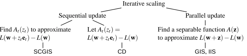
Iterative scaling Sequential update
Find At(zt)to approximate
L(w+ztet)−L(w)
SCGIS
Let At(zt) =
L(w+ztet)−L(w)
CD
Parallel update Find a separable function A(z) to approximate L(w+z)−L(w)
GIS,IIS
Figure 1: An illustration of various iterative scaling methods.
ISmethods because they remain one of the most used approaches to train Maxent. This fact can be easily seen from popular NLP software. The Stanford Log-linear POS Tagger1 supports two optimization methods, where one isIIS. The OpenNLP Maxent package (Baldridge et al., 2001) provides only one optimization method, which isGIS.
This paper is organized as follows. In Section 2, we present a unified framework for IS/CD
methods and give theoretical results. Section 3 proposes a new CDmethod. Its advantages over existingIS/CDmethods are discussed. In Section 4, we investigate some implementation issues for
IS/CD methods. Section 5 presents experimental results. With a careful implementation, our CD
outperformsISand quasi-Newton techniques. Finally, Section 6 gives discussion and conclusions. Part of this work appears in a short conference paper (Huang et al., 2009).
Notation X , Y , and n are the numbers of contexts, class labels, and features, respectively. The total number of nonzeros in training data and the average number of nonzeros per feature are re-spectively
#nz≡
∑
x,yt: ft(
∑
x,y)6=01 and ¯l≡#nz
n . (4)
In this paper, we assume non-negative feature values:
ft(x,y)≥0,∀t,x,y. (5)
Most NLP applications have non-negative feature values. All existingISmethods use this property.
2. A Framework for Iterative Scaling and Coordinate Descent Methods
An important characteristic ofIS andCD methods is that they solve a one-variable optimization problem and then modify the corresponding element in w. Conceptually, the one-variable sub-problem is related to the function reduction
L(w+ztet)−L(w), where et ≡[0, . . . ,0
| {z }
t−1
,1,0, . . . ,0]T. Then IS methods differ in how they approximate the function
reduction. They can also be categorized according to whether w’s components are updated in a sequential or parallel way. In this section, we create a framework for these methods. A hierarchical illustration of the framework is in Figure 1.
2.1 The Framework
To introduce the framework, we separately discuss coordinate descent methods according to whether w is sequentially or parallely updated.
2.1.1 SEQUENTIAL UPDATE
For a sequential-update algorithm, once a one-variable sub-problem is solved, the corresponding element in w is updated. The new w is then used to construct the next sub-problem. The procedure is sketched in Algorithm 1. If the t-th component is selected for update, a sequentialIS method solves the following one-variable sub-problem:
min zt
At(zt),
where At(zt)is twice differentiable and bounds the function difference:
At(zt)≥L(w+ztet)−L(w),∀zt. (6)
We hope that by minimizing At(zt), the resulting L(w+ztet)can be smaller than L(w). However, (6) is not enough to ensure this property, so we impose an additional condition
At(0) =0 (7)
on the approximate function At(zt). The explanation below shows that we can strictly decrease the function value. If A′t(0)6=0 and assume ¯zt≡arg minztAt(zt)exists, with the condition At(0) =0,
we have At(¯zt)<0. This property and (6) then imply L(w+¯ztet)<L(w). If A′t(0) =0, we can prove that∇tL(w) =0,2where∇tL(w) =∂L(w)/∂wt.In this situation, the convexity of L(w)and
∇tL(w) =0 imply that we cannot decrease the function value by modifying wt, so we should move on to modify other components of w.
ACDmethod can be viewed as a sequential-updateISmethod. Its approximate function At(zt) is simply the function difference:
AtCD(zt) =L(w+ztet)−L(w). (8)
OtherISmethods consider approximations so that At(zt)is simpler for minimization. More details are in Section 2.2. Note that the name “sequential” comes from the fact that each sub-problem At(zt) depends on w obtained from the previous update. Therefore, sub-problems must be sequentially solved.
2.1.2 PARALLELUPDATE
A parallel-updateISmethod simultaneously constructs n independent one-variable sub-problems. After (approximately) solving all of them, the whole vector w is updated. Algorithm 2 gives the procedure. The function A(z),z∈Rn, is an approximation of L(w+z)−L(w)satisfying
A(z)≥L(w+z)−L(w), ∀z, A(0) =0, and A(z) = n
∑
t=1
At(zt). (9)
2. Define a function D(zt)≡A(zt)−(L(w+ztet)−L(w)). We have D′(0) =A′(0)−∇tL(w). If∇tL(w)6=0 and At′(0) =0, then D′(0)6=0. Since D(0) =0, we can find a ztsuch that A(zt)−(L(w+ztet)−L(w))<0, a contradiction
Algorithm 1 A sequential-updateISmethod While w is not optimal
For t=1, . . . ,n
1. Find an approximate function At(zt)satisfying (6)-(7). 2. Approximately solve minztAt(zt)to get ¯zt.
3. wt←wt+¯zt.
Algorithm 2 A parallel-updateISmethod While w is not optimal
1. Find approximate functions At(zt)∀zt satisfying (9). 2. For t=1, . . . ,n
Approximately solve minztAt(zt)to get ¯zt.
3. For t=1, . . . ,n wt←wt+¯zt.
The first two conditions are similar to (6) and (7). By a similar argument, we can ensure that the function value is strictly decreasing. The last condition indicates that A(z)is separable, so
min
z A(z) =
n
∑
t=1 min
zt
At(zt).
That is, we can minimize At(zt), ∀zt simultaneously, and then update wt ∀t together. We show in Section 4 that a parallel-update method possesses some nicer implementation properties than a sequential method. However, as sequential approaches update w as soon as a sub-problem is solved, they often converge faster than parallel methods.
If A(z) satisfies (9), taking z=ztet implies that (6) and (7) hold for At(zt), ∀t=1, . . . ,n. A parallel-update method could thus be transformed to a sequential-update method using the same approximate function. Contrarily, a sequential-update algorithm cannot be directly transformed to a parallel-update method because the summation of the inequality in (6) does not imply (9).
2.2 Existing Iterative Scaling Methods
We introduceGIS,IISandSCGISvia the proposed framework. GISandIISuse a parallel update, but
SCGISis sequential. Their approximate functions aim to bound the change of the function values
L(w+z)−L(w) =
∑
x ˜
P(x)logTw+z(x)
Tw(x)
+
∑
t
Qt(zt), (10)
where Tw(x)is defined in (1) and
Qt(zt)≡
2wtzt+z2t
2σ2 −ztP˜(ft). (11) ThenGIS,IISandSCGISuse similar inequalities to get approximate functions. With
Tw+z(x)
Tw(x)
=∑ySw+z(x,y)
Tw(x)
= ∑ySw(x,y) e
∑tztft(x,y)
Tw(x)
=
∑
y
they apply logα≤α−1∀α>0 and∑yPw(y|x) =1 to get
(10)≤
∑
tQt(zt) +
∑
x˜
P(x)
∑
y
Pw(y|x)e∑tztft(x,y)−1
!
=
∑
t
Qt(zt) +
∑
x,y ˜P(x)Pw(y|x)
e∑tztft(x,y)−1.
(12)
GISdefines
f#≡max
x,y f
#(x,y), f#(x,y)
≡
∑
t
ft(x,y),
and adds a feature fn+1(x,y)≡ f#−f#(x,y) with zn+1 =0. Using Jensen’s inequality and the assumption of non-negative feature values (5),
e∑nt=1ztft(x,y)=e∑ n+1 t=1 ft
(x,y) f # ztf
#
(13)
≤
n+1
∑
t=1
ft(x,y)
f# e
ztf# =
n
∑
t=1
ft(x,y)
f# e
ztf#+ f
#−f#(x,y)
f# =
n
∑
t=1
eztf#−1
f# ft(x,y)
!
+1.
Substituting (13) into (12), the approximate function ofGISis
AGIS(z) =
∑
tQt(zt) +
∑
x,y ˜P(x)Pw(y|x)
∑
t
eztf#−1
f# ft(x,y)
!
.
Then we obtain n independent one-variable functions:
AGISt (zt) =Qt(zt) +
eztf#−1
f#
∑
x,y ˜
P(x)Pw(y|x)ft(x,y).
IISassumes ft(x,y)≥0 and applies Jensen’s inequality
e∑tztft(x,y)=e∑t ft(x,y) f #(x,y)ztf
#(x,y)
≤
∑
t
ft(x,y)
f#(x,y)e ztf#(x,y)
on (12) to get the approximate function
AIISt (zt) =Qt(zt) +
∑
x,y ˜P(x)Pw(y|x)ft(x,y)
eztf#(x,y)−1
f#(x,y) .
SCGISis a sequential-update algorithm. It replaces f#inGISwith
ft#≡max
x,y ft(x,y). (14)
Using ztet as z in (10), a derivation similar to (13) gives
eztft(x,y)≤ ft(x,y)
ft#
eztft#+ f
#
t −ft(x,y)
ft#
The approximate function ofSCGISis
AtSCGIS(zt) =Qt(zt) +
eztft#−1
f# t
∑
x,y˜
P(x)Pw(y|x)ft(x,y).
As a comparison, we expand ACDt (zt)in (8) to the following form:
AtCD(zt) =Qt(zt) +
∑
x˜
P(x)logTw+ztet(x)
Tw(x)
(16)
=Qt(zt) +
∑
x˜
P(x)log 1+
∑
y
Pw(y|x)(eztft(x,y)−1)
!
, (17)
where (17) is from (1) and
Sw+ztet(x,y) =Sw(x,y)e
ztft(x,y), (18)
Tw+ztet(x) =Tw(x) +
∑
y
Sw(x,y)(eztft(x,y)−1). (19)
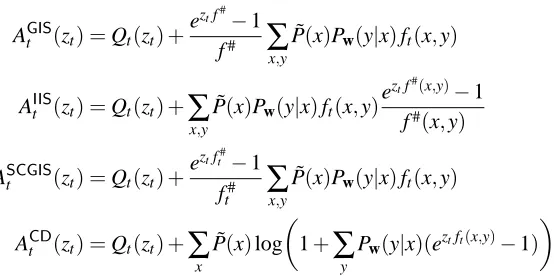
A summary of approximate functions ofISandCDmethods is in Table 1.
2.3 Convergence of Iterative Scaling and Coordinate Descent Methods
The convergence of CD methods has been well studied (e.g., Bertsekas, 1999; Luo and Tseng, 1992). However, for methods likeISwhich use only an approximate function to bound the function difference, the convergence is less studied. In this section, we generalize the linear convergence proof in Chang et al. (2008) to show the convergence ofISandCDmethods. To begin, we consider any convex and differentiable function L: Rn→R satisfying the following conditions in the set
U={w|L(w)≤L(w0)}, (20)
where w0is the initial point of anIS/CDalgorithm:
1. ∇L is bi-Lipschitz: there are two positive constantsτmaxandτminsuch that for any u,v∈U ,
τminku−vk ≤ k∇L(u)−∇L(v)k ≤τmaxku−vk. (21)
2. Quadratic bound property: there is a constant K>0 such that for any u,v∈U
|L(u)−L(v)−∇L(v)T(u−v)| ≤Kku−vk2. (22)
The following theorem proves that (3) satisfies these two conditions.
Theorem 1 L(w)defined in (3) satisfies (21) and (22).
The proof is in Section 7.1.
AGISt (zt) =Qt(zt) +
eztf#−1
f#
∑
x,y ˜
P(x)Pw(y|x)ft(x,y)
AIISt (zt) =Qt(zt) +
∑
x,y ˜P(x)Pw(y|x)ft(x,y)
eztf#(x,y)−1
f#(x,y)
ASCGISt (zt) =Qt(zt) +
eztft#−1
ft#
∑
x,y ˜P(x)Pw(y|x)ft(x,y)
ACDt (zt) =Qt(zt) +
∑
x˜
P(x)log
1+
∑
yPw(y|x)(eztft(x,y)−1)
Table 1: Approximate functions ofISandCDmethods.
Theorem 2 Consider Algorithm 1 or 2 to minimize a convex and twice differentiable function L(w).
Assume L(w)attains a unique global minimum w∗ and L(w)satisfies (21)-(22). If the algorithm
satisfies
kwk+1−wkk ≥ ηk∇L(wk)k, (23)
L(wk+1)−L(wk) ≤ −νkwk+1−wkk2, (24)
for some positive constantsηandν, then the sequence{wk} generated by the algorithm linearly
converges. That is, there is a constant µ∈(0,1)such that
L(wk+1)−L(w∗)≤(1−µ)(L(wk)−L(w∗)),∀k.
The proof is in Section 7.2. Note that this theorem is not restricted to L(w)in (3). Next, we show that
IS/CDmethods discussed in this paper satisfy (23)-(24), so they all possess the linear convergence property.
Theorem 3 Consider L(w) defined in (3) and assume At(zt) is exactly minimized in GIS, IIS,
SCGIS, orCD. Then{wk}satisfies (23)-(24).
The proof is in Section 7.3.
2.4 Solving One-variable Sub-problems
After generating approximate functions, GIS, IIS,SCGIS andCD need to minimize one-variable sub-problems. In general, the approximate function possesses a unique global minimum. We do not discuss some rare situations where this property does not hold (for example, minzt A
GIS
t (zt)has an optimal solution zt =−∞if ˜P(ft) =0 and the regularization term is not considered).
Without the regularization term, by A′t(zt) =0,GISandSCGISboth have a simple closed-form solution of the sub-problem:
zt = 1
fslog
˜
P(ft)
∑x,yP˜(x)Pw(y|x)ft(x,y)
!
, where fs≡
(
f#if s isGIS,
ForIIS, the term eztf#(x,y)in AIIS
t (zt)depends on x and y, so it does not have a closed-form solution.
CDdoes not have a closed-form solution either.
With the regularization term, the sub-problems no longer have a closed-form solution. While many optimization methods can be applied, in this section we analyze the complexity of using the Newton method to solve one-variable sub-problems. The Newton method minimizes Ast(zt)by iteratively updating zt:
zt←zt−Ast′(zt)/Ats′′(zt), (26)
where s indicates anISor aCDmethod. This iterative procedure may diverge, so we often need a line search procedure to ensure the function value is decreasing (Fletcher, 1987, p. 47). Due to the many variants of line searches, here we discuss only the cost for finding the Newton direction. The Newton directions ofGISandSCGISare similar:
−A
s t′(zt)
Ast′′(zt)
=− Q
′
t(zt) +eztf
s
∑x,yP˜(x)Pw(y|x)ft(x,y)
Qt′′(zt) +fseztf
s
∑x,yP˜(x)Pw(y|x)ft(x,y)
, (27)
where fsis defined in (25). ForIIS, the Newton direction is:
−A
IIS
t ′(zt)
AIISt ′′(zt)
=− Q
′
t(zt) +∑x,yP˜(x)Pw(y|x)ft(x,y)eztf
#(x,y)
Qt′′(zt) +∑x,yP˜(x)Pw(y|x)ft(x,y)f#(x,y)eztf
#(x,y). (28)
The Newton directions ofCDis:
−A
CD
t ′(zt)
AtCD′′(zt)
, (29)
where
ACDt ′(zt) = Q′t(zt) +
∑
x,y ˜P(x)Pw+ztet(y|x)ft(x,y), (30)
ACDt ′′(zt) = Q′′t(zt) +
∑
x,y ˜P(x)Pw+ztet(y|x)ft(x,y)
2
−
∑
x ˜
P(x)
∑
y
Pw+ztet(y|x)ft(x,y)
!2
. (31)
Eqs. (27)-(28) can be easily obtained using formulas in Table 1. We show details of deriving (30)-(31) in Section 7.4.
We separate the complexity analysis to two parts. One is on calculating of Pw(y|x)∀x,y, and the
other is on the remaining operations.
For Pw(y|x) =Sw(x,y)/Tw(x), parallel-update approaches calculate it once every n sub-problems. To get Sw(x,y)∀x,y, the operation
∑
t
wtft(x,y) ∀x,y
needs O(#nz)time. If XY ≤#nz, the cost for obtaining Pw(y|x),∀x,y is O(#nz), where X and Y are
respectively the numbers of contexts and labels.3 Therefore, on average each sub-problem shares
O(#nz/n) =O(¯l)cost. For sequential-update methods, they expensively update Pw(y|x)after every 3. If XY>#nz, one can calculate ewtft(x,y),∀f
t(x,y)6=0 and then the product∏t: ft(x,y)6=0e
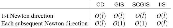
CD GIS SCGIS IIS
1st Newton direction O(¯l) O(¯l) O(¯l) O(¯l) Each subsequent Newton direction O(¯l) O(1) O(1) O(¯l)
Table 2: Cost for finding Newton directions if the Newton method is used to minimize At(zt).
sub-problem. A trick to trade memory for time is to store all Sw(x,y)and Tw(x), and use (18) and
(19). Since Sw+ztet(x,y) =Sw(x,y), if ft(x,y) =0, this procedure reduces the number of operations
from the O(#nz)operations to O(¯l). However, it needs O(XY)extra spaces to store all Sw(x,y)and
Tw(x). This trick has been used in theSCGISmethod (Goodman, 2002).
From (27) and (28), all remaining operations ofGIS,IIS, andSCGISinvolve the calculation of
∑
x,y ˜
P(x)Pw(y|x)ft(x,y)(a function of zt), (32)
which needs O(¯l)under a fixed t. ForGISandSCGIS, since the function of ztin (32) is independent
of x,y, we can calculate and store∑x,yP˜(x)Pw(y|x)ft(x,y)in the first Newton iteration. Therefore,
the overall cost (including calculating Pw(y|x)) is O(¯l) for the first Newton iteration and O(1)for
each subsequent iteration. ForIIS, because eztf#(x,y)in (28) depends on x and y, we need O(¯l)for
every Newton direction. For CD, it calculates Pw+ztet(y|x) for every zt, so the cost per Newton
direction is O(¯l). We summarize the cost for solving sub-problems ofGIS,SCGIS,IISandCDin Table 2.
2.5 Related Work
Our framework forISmethods includes two important components:
1. Approximate L(w+ztet)−L(w)or L(w+z)−L(w)to obtain functions At(zt). 2. Sequentially or parallely minimize approximate functions.
Each component has been well discussed in many places. However, ours may be the first to investi-gateISmethods in detail. Below we discuss some related work.
The closest work to our framework might be Lange et al. (2000) from the statistics community. They discuss “optimization transfer” algorithms which construct At(zt)or A(z)satisfying conditions similar to (6)-(7) or (9). However, they do not require one-variable sub-problems, so A(z) of a parallel-update method may be non-separable. They discuss that “optimization transfer” algorithms can be traced back to EM (Expectation Maximization). In their paper, the function At(zt)or A(z)is called a “surrogate” function or a “majorizing” function. Some also call it an “auxiliary” function. Lange et al. (2000) further discuss several ways to construct A(z), where Jensen’s inequality used in (13) is one of them. An extension along this line of research is by Zhang et al. (2007).
The concept of sequential- and parallel-update algorithms is well known in many subjects. For example, these algorithms are used in iterative methods for solving linear systems (Jacobi and Gauss-Seidel methods). Some recent machine learning works which mention them include, for example, Collins et al. (2002) and Dud´ık et al. (2004). Dud´ık et al. (2004) propose a variant ofIS
algorithms using certain approximate functions. Their sequential methods greedily choose coordi-nates minimizing At(zt), while ours in Section 2.1.1 chooses coordinates cyclicly.
Regarding the convergence, if the sub-problem has a closed-form solution like (25), it is easy to apply the result in Lange et al. (2000). However, the case with regularization is more complicated. For example, Dud´ık et al. (2004) point out that Goodman (2002) does not give a “complete proof of convergence.” Note that the strict decrease of function values following conditions (6)-(7) or (9) does not imply the convergence to the optimal function value. In Section 2.3, we prove not only the global convergence but also the linear convergence for a general class ofIS/CDmethods.
3. Comparison and a New Coordinate Descent Method
Using the framework in Section 2, we compareCD andISmethods in this section. Based on the comparison, we propose a new and fastCDmethod.
3.1 Comparison of Iterative Scaling and Coordinate Descent Methods AnISorCDmethod falls into a place between two extreme designs:
At(zt)a loose bound
⇐⇒ At(zt)a tight bound
Easy to minimize At(zt) Hard to minimize At(zt)
That is, there is a tradeoff between the tightness to bound the function difference and the hardness to solve the sub-problem. To check howISandCDmethods fit into this explanation, we obtain the following relationship of their approximate functions:
AtCD(zt)≤A
SCGIS
t (zt)≤A
GIS
t (zt),
AtCD(zt)≤A
IIS
t (zt)≤A
GIS
t (zt) ∀zt.
(33)
The derivation is in Section 7.5. From (33),CDconsiders more accurate sub-problems thanSCGIS
andGIS. However, when solving the sub-problem, from Table 2,CD’s each Newton step takes more time. The same situation occurs in comparingIISandGIS.
The above discussion indicates that while a tight At(zt)can give faster convergence by handling fewer sub-problems, the total time may not be less due to the higher cost of each sub-problem.
3.2 A Fast Coordinate Descent Method
Based on the discussion in Section 3.1, we develop aCDmethod which is cheaper in solving each sub-problem but still enjoys fast final convergence. This method is modified from Chang et al. (2008), aCDapproach for linear SVM. They approximately minimize ACDt (zt)by applying only one Newton iteration. This approach is a truncated Newton method: In the early stage of the coordinate descent method, we roughly minimize AtCD(zt)but in the final stage, one Newton update can quite accurately solve the sub-problem. The Newton direction at zt=0 is
d=−A
CD
t ′(0)
ACDt ′′(0). (34)
Algorithm 3 A fast coordinate descent method for Maxent
• Chooseβ∈(0,1)andγ∈(0,1/2). Give initial w and calculate Sw(x,y),Tw(x),∀x,y.
• While w is not optimal – For t=1, . . . ,n
1. Calculate the Newton direction
d=−AtCD′(0)/ACDt ′′(0)
= − ∑x,yP˜(x)Pw(y|x)ft(x,y) + wt
σ2
∑x,yP˜(x)Pw(y|x)ft(x,y)2−∑xP˜(x) ∑yPw(y|x)ft(x,y)
2
+ 1
σ2
,
where
Pw(y|x) =
Sw(x,y)
Tw(x)
.
2. Whileλ=1,β,β2, . . . (a) Let zt =λd
(b) Calculate
ACDt (zt) =Qt(zt) +
∑
x˜
P(x)log 1+
∑
y
Sw(x,y)
Tw(x)
(eztft(x,y)−1)
!
(c) If ACDt (zt)≤γztAtCD′(0), then break. 3. wt ←wt+zt
4. Update Sw(x,y)and Tw(x)∀x,y by (18)-(19)
decrease condition:
AtCD(zt)−AtCD(0) =A
CD
t (zt)≤γztAtCD
′
(0)≤0, (35)
whereγis a constant in(0,1/2). Note that ztACDt ′(0)is negative under the definition of d in (34). Instead of (35), Grippo and Sciandrone (1999) and Chang et al. (2008) use
ACDt (zt)≤ −γz2t (36)
as the sufficient decrease condition. We prefer (35) as it is scale-invariant. That is, if ACDt is linearly scaled, then (35) holds under the sameγ. In contrast,γin (36) may need to be changed. To findλ for (35), a simple way is by sequentially checkingλ=1,β,β2, . . ., whereβ∈(0,1). We chooseβas 0.5 for experiments. The following theorem proves that the condition (35) can always be satisfied.
Theorem 4 Given the Newton direction d as in (34). There is ¯λ>0 such that zt =λd satisfies (35)
for all 0≤λ<¯λ.
The proof is in Section 7.6. The newCDprocedure is in Algorithm 3. In the rest of this paper, we refer toCDas this new algorithm.
Theorem 5 Algorithm 3 satisfies (23)-(24) and linearly converges to the global optimum of (3). As evaluating ACDt (zt)via (17)-(19) needs O(¯l)time, the line search procedure takes
O(¯l)×(# line search steps).
This causes the cost of solving a sub-problem higher than that ofGIS/SCGIS(see Table 2). Fortu-nately, we show that near the optimum, the line search procedure needs only one step:
Theorem 6 In a neighborhood of the optimal solution, the Newton direction d defined in (34)
sat-isfies the sufficient decrease condition (35) withλ=1.
The proof is in Section 7.8. If the line search procedure succeeds atλ=1, then the cost for each sub-problem is similar to that ofGISandSCGIS.
Next we show that near the optimum, one Newton direction ofCD’s tight ACDt (zt) already re-duces the objective function L(w)more rapidly than directions by exactly minimizing a loose At(zt) ofGIS,IISorSCGIS. Thus Algorithm 3 has faster final convergence thanGIS,IIS, orSCGIS.
Theorem 7 Assume w∗ is the global optimum of (3). There is anε>0 such that the following
result holds. For any w satisfyingkw−w∗k ≤ε, if we select an index t and generate directions
d=−AtCD′(0)/AtCD′′(0) and ds=arg min zt
Ast(zt), s=GIS,IISorSCGIS, (37)
then
δt(d)<min
δt(d
GIS
),δt(d
IIS
),δt(d
SCGIS
),
where
δt(zt)≡L(w+ztet)−L(w).
The proof is in Section 7.9. Theorems 6 and 7 show that Algorithm 3 improves upon the traditional
CD by approximately solving sub-problems, while still maintaining fast convergence. That is, it attempts to take both advantages of the two designs mentioned in Section 3.1.
3.2.1 EFFICIENT LINE SEARCH
We propose a technique to speed up the line search procedure. We derive a function ¯ACDt (zt)so that it is cheaper to calculate than AtCD(zt)and satisfies ¯ACDt (zt)≥AtCD(zt)∀zt.Then,
¯
ACDt (zt)≤γztA
CD
t
′
(0) (38)
implies (35), so we can save time by replacing step 2 of Algorithm 3 with 2’. Whileλ=1,β,β2, . . .
(a) Let zt=λd
(b) Calculate ¯ACDt (zt) (c) If ¯ACDt (zt)≤γztACDt
′
(0), then break. (d) Calculate ACDt (zt)
We assume non-negative feature values and obtain
¯
ACDt (zt)≡Qt(zt) +P˜tlog 1+
eztft#−1
f# t P˜t
∑
x,y˜
P(x)Pw(y|x)ft(x,y)
!
, (39)
where ft#is defined in (14), ˜
Pt≡
∑
Ωt
˜
P(x), and Ωt ≡ {x :∃y such that ft(x,y)6=0}. (40)
The derivation is in Section 7.10. Because
∑
x,y ˜
P(x)Pw(y|x)ft(x,y),t=1, . . . ,n (41)
are available from finding ACDt ′(0), getting ¯ACDt (zt)and checking (38) take only O(1), smaller than
O(¯l)for (35). Using logα≤α−1∀α>0, it is easy to see that ¯
ACDt (zt)≤A
SCGIS
t (zt),∀zt.
Therefore, we can simply replace ASCGISt (zt)of theSCGISmethod with ¯ACDt (zt)to have a newIS method.
4. Implementation Issues
In this section we analyze some implementation issues ofISandCDmethods.
4.1 Row Versus Column Format
In many Maxent applications, data are sparse with few nonzero ft(x,y). We store such data by a sparse matrix. Among many ways to implement sparse matrices, two common ones are “row format” and “column format.” For the row format, each (x,y) corresponds to a list of nonzero
ft(x,y), while for the column format, each feature t is associated with a list of (x,y). The loop to access data in the row format is (x,y)→t, while for the column format it is t →(x,y). By
(x,y)→t we mean that the outer loop goes through(x,y) values and for each (x,y), there is an
inner loop for a list of feature values. For sequential-update algorithms such as SCGISand CD, as we need to maintain Sw(x,y)∀x,y via (18) after solving the t-th sub-problem, an easy access of
t’s corresponding(x,y) elements is essential. Therefore, the column format is more suitable. In
contrast, parallel-update methods can use either row or column formats. ForGIS, we can store all n elements of (41) before solving n sub-problems by (25) or (27). The calculation of (41) can be done by using the row format and a loop of(x,y)→t. For IIS, an implementation by the row format is more complicated due to the eztf#(x,y)term in AIIS
t (zt). Take the Newton method to solve the sub-problem as an example. We can calculate and store (28) for all t=1, . . . ,n by a loop of(x,y)→t.
That is, n Newton directions are obtained together before conducting n updates.
4.2 Memory Requirement
For sequential-update methods, to save the computational time of calculating Pw(y|x), we use
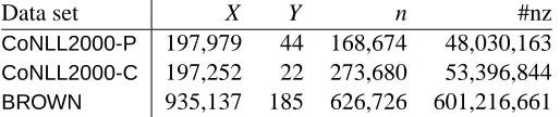
Data set X Y n #nz
CoNLL2000-P 197,979 44 168,674 48,030,163
CoNLL2000-C 197,252 22 273,680 53,396,844
BROWN 935,137 185 626,726 601,216,661
Table 3: Statistics of NLP data (0/1 features). X : number of contexts, Y : number of class labels, n: number of features, and #nz: number of total non-zero feature values; see (4).
methods, they also need O(XY)spaces if using the column format: To calculate e∑twtft(x,y)∀x,y via
a loop of t→(x,y), we need O(XY) positions to store∑twtft(x,y)∀x,y. In contrast, if using the row format, the loop is x→y→t, so for each fixed x, we need only O(Y)spaces to store S(x,y)∀y
and then obtain Tw(x). This advantage makes the parallel update a viable approach if Y (the number
of labels) is very large.
4.3 Number of exp and log Operations
Many exp/log operations are needed in training a Maxent model. On most computers, exp/log operations are much more expensive than multiplications/divisions. It is important to analyze the number of exp/log operations inISandCDmethods.
We first discuss the number of exp operations. A simple check of (27)-(31) shows that the numbers are the same as those in Table 2. IISandCDneed O(¯l)exp operations for every Newton direction because they calculate eztf#(x,y)in (28) and eztft(x,y)in (17), respectively.CDvia Algorithm
3 takes only one Newton iteration, but each line search step also needs O(¯l) exp operations. If feature values are binary, eztft(x,y)in (17) becomes ezt, a value independent of x,y. Thus the number
of exp operations is significantly reduced from O(¯l)to O(1). This property implies that Algorithm 3 is more efficient if data are binary valued. In Section 5, we will confirm this result through experiments.
Regarding log operations, GIS,IIS andSCGIS need none as they remove the log function in
At(zt). CDvia Algorithm 3 keeps log in AtCD(zt)and requires O(|Ωt|) log operations at each line search step, whereΩt is defined in (40).
4.4 Permutation of Indices in Solving Sub-problems
For sequential-update methods, one does not have to follow a cyclic way to update w1, . . . ,wn. Chang et al. (2008) report that in their CD method, a permutation of {1, . . . ,n} as the order for solving n sub-problems leads to faster convergence. For sequential-updateISmethods adopting this strategy, the linear convergence in Theorem 2 still holds.
5. Experiments
In this section, we compareIS/CDmethods to reconfirm properties discussed in earlier sections. We consider two types of data for NLP (Natural Language Processing) applications. One is Maxent for 0/1-featured data and the other is Maxent (logistic regression) for document data with non-negative real-valued features. Programs used for experiments in this paper are online available at
0 50 100 150 10−3 10−2 10−1 100 101 102
Training Time (s)
Relative function value difference
GIS SCGIS CD LBFGS TRON (a)CoNLL2000-P
0 50 100 150 200
10−2
10−1
100
101
102
Training Time (s)
Relative function value difference
GIS SCGIS CD LBFGS TRON (b)CoNLL2000-C
0 500 1000 1500 2000 10−2
10−1 100
101
Training Time (s)
Relative function value difference
GIS SCGIS CD LBFGS TRON (c) BROWN
0 50 100 150
101
102
103
Training Time (s)
|| ∇ L(w)|| GIS SCGIS CD LBFGS TRON (d)CoNLL2000-P
0 50 100 150 200
101
102
103
Training Time (s)
|| ∇ L(w)|| GIS SCGIS CD LBFGS TRON (e) CoNLL2000-C
0 500 1000 1500 2000 102
103
104
Training Time (s)
|| ∇ L(w)|| GIS SCGIS CD LBFGS TRON (f) BROWN
0 50 100 150
94 94.5 95 95.5 96 96.5 97 97.5 98
Training Time (s)
Testing Accuracy GIS SCGIS CD LBFGS TRON (g)CoNLL2000-P
0 50 100 150 200
90 90.5 91 91.5 92 92.5 93 93.5
Training Time (s)
F1 measure GIS SCGIS CD LBFGS TRON (h)CoNLL2000-C
0 500 1000 1500 2000 94 94.5 95 95.5 96 96.5 97
Training Time (s)
Testing Accuracy GIS SCGIS CD LBFGS TRON (i)BROWN
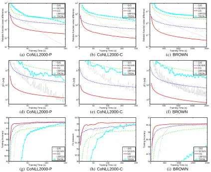
Figure 2: Results on 0/1-featured data. The first row shows time versus the relative function dif-ference (42). The second and third rows showk∇L(w)kand testing performances along time, respectively. Time is in seconds.
5.1 Maxent for 0/1-featured Data in NLP
We apply Maxent models to part of speech (POS) tagging and chunking tasks. In POS tagging, we mark a POS tag to the word in a text based on both its definition and context. In a chunking task, we divide a text into syntactically correlated parts of words. That is, given words in a sentence annotated with POS tags, we label each word with a chunk tag. Other learning models such as CRF (Conditional Random Fields) may outperform Maxent for these NLP applications. However, we do not consider other learning models as the focus of this paper is to studyISmethods for Maxent.
We use CoNLL2000 shared task data4 for chunking and POS tagging, and BROWN corpus5 for POS tagging. CoNLL2000-PindicatesCoNLL2000for POS tagging, andCoNLL2000-Cmeans
CoNLL2000for chunking. CoNLL2000data consist of Sections 15-18 of the Wall Street Journal corpus as training data and Section 20 as testing data. For theBROWNcorpus, we randomly
lect four-fifth articles for training and use the rest for testing. We omit the stylistic tag modifiers “fw,”“tl,”“nc,”and “hl,” so the number of labels is reduced from 472 to 185. Our implementation is built upon the OpenNLP package (Baldridge et al., 2001). We use the default setting of OpenNLP to extract binary features (0/1 values) suggested by Ratnaparkhi (1998). The OpenNLP imple-mentation assumes that each feature index t corresponds to a unique label y. In prediction, we approximately maximize the probability of tag sequences to the word sequences by a beam search (Ratnaparkhi, 1998). Table 3 lists the statistics of data sets.
We implement the following methods for comparisons.
1. GIS and SCGIS: To minimize At(zt), we run Newton updates (without line search) until
|A′t(zt)| ≤10−5. We can afford many Newton iterations because, according to Table 2, each Newton direction costs only O(1)time.
2. CD: the coordinate descent method proposed in Section 3.2.
3. LBFGS: a limited memory quasi Newton method for general unconstrained optimization problems (Liu and Nocedal, 1989).
4. TRON: a trust region Newton method for logistic regression (Lin et al., 2008). We extend the method for Maxent.
We considerLBFGSas Malouf (2002) reports that it is better than other approaches including
GISandIIS. Lin et al. (2008) show thatTRONis faster thanLBFGSfor document classification, so we includeTRONfor comparison. We excludeIISbecause of its higher cost per Newton direction thanGIS/SCGIS(see Table 2). Indeed Malouf (2002) reports thatGISoutperformsIIS. Our imple-mentation of all methods takes the property of 0/1 features. We use the regularization parameter
σ2=10 as under this value Maxent models achieve good testing performances. We setβ=0.5 and
γ=0.001 for the line search procedure (35) inCD. The initial w of all methods is 0.
We begin at checking time versus the relative difference of the function value to the optimum:
L(w)−L(w∗)
L(w∗) , (42)
where w∗is the optimal solution of (3). As w∗is not available, we obtain a reference point satisfying
k∇L(w)k ≤0.01. Results are in the first row of Figure 2. Next, we check these methods’ gradient values. As k∇L(w)k=0 implies that w is the global minimum, usually k∇L(w)k is used in a stopping condition. The second row of Figure 2 shows time versusk∇L(w)k. We are also interested in the time needed to achieve a reasonable testing result. We measure the performance of POS tagging by accuracy and chunking by F1 measure. The third row of Figure 2 presents the testing accuracy/F1 versus training time. Note that (42) andk∇L(w)kin Figure 2 are both log scaled.
We give some observations from Figure 2. Among the threeIS/CDmethods compared, the new
CDapproach discussed in Section 3.2 is the fastest. SCGIScomes the second, whileGISis the last. This result is consistent with the tightness of their approximate functions; see (33). RegardingIS/CD
methods versusLBFGS/TRON, the threeIS/CDmethods more quickly decrease the function value in the beginning, butLBFGS has faster final convergence. In fact, if we draw figures with longer training time, TRON’s final convergence is the fastest. This result is reasonable as LBFGS and
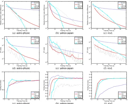
Problem l n #nz σ2
astro-physic 62,369 99,757 4,834,550 8l
yahoo-japan 176,203 832,026 23,506,415 4l
rcv1 677,399 47,236 49,556,258 8l
Table 4: Statistics of document data (real-valued features). l: number of instances, n: number of features, #nz: number of total non-zero feature values, and σ2: best regularization parameter from five-fold cross validation.
reasonable model quickly (IS/CDmethods) or accurately minimizing the function (LBFGS/TRON). PracticallyCD/ISmay be more useful as they reach the final testing accuracy rapidly. Finally, we compare LBFGSandTRON. Surprisingly, LBFGSoutperformsTRON, a result opposite to that in Lin et al. (2008). We do not have a clear explanation yet. A difference is that Lin et al. (2008) deal with document data of real-valued features, but here we have 0/1-featured NLP applications. Therefore, one should always be careful that for the same approaches, observations made on one type of data may not extend to another.
In Section 4, we discussed a strategy of permuting n sub-problems to speed up the convergence of sequential-updateISmethods. However, in training Maxent models for 0/1-featured NLP data, with/without permutation gives similar performances. We find that this strategy tends to work better if features are related. Hence we suspect that features used in POS tagging or chunking tasks are less correlated than those in documents and the order of sub-problems is not very important.
5.2 Maxent (Logistic Regression) for Document Classification
In this section, we experiment with logistic regression on document data with non-negative real-valued features. Chang et al. (2008) report that theirCDmethod is very efficient for linear SVM, but is slightly less effective for logistic regression. They attribute the reason to that logistic regression requires expensive exp/log operations. In Section 4, we show that for 0/1 features, the number of
ISmethods’ exp operations is smaller. Experiments here help to check ifIS/CDmethods are more suitable for 0/1 features than real values.
Logistic regression is a special case of maximum entropy with two labels+1 and−1. Consider training data{¯xi,y¯i}li=1,¯xi∈Rn,y¯i={1,−1}. Assume ¯xit ≥0, ∀i,t. We set the feature ft(xi,y)as
ft(xi,y) =
(
¯
xit if y=1, 0 if y=−1,
where xidenotes the index of the i-th training instance ¯xi. Then
Sw(xi,y) =e∑twtft(xi,y)=
(
ewT¯xi if y=1,
1 if y=−1,
and
Pw(y|xi) =
Sw(xi,y)
Tw(xi)
= 1
1+e−ywT¯x
i. (43)
From (2) and (43),
L(w) = 2σ12∑tw2t +1l∑ilog
1+e−y¯iwT¯xi
0 0.5 1 1.5 2 2.5 3 3.5 4 10−4 10−3 10−2 10−1 100 101
Training Time (s)
Relative function value difference
SCGIS CD LBFGS TRON
(a) astro-physic
0 10 20 30 40 50
10−4
10−3
10−2
10−1
100
Training Time (s)
Relative function value difference
SCGIS CD LBFGS TRON
(b)yahoo-japan
0 10 20 30 40 50 60 10−4 10−3 10−2 10−1 100 101
Training Time (s)
Relative function value difference
SCGIS CD LBFGS TRON
(c)rcv1
0 0.5 1 1.5 2 2.5 3 3.5 4 10−5
10−4
10−3
10−2
Training Time (s)
|| ∇ L(w)|| SCGIS CD LBFGS TRON (d)astro-physic
0 10 20 30 40 50
10−5
10−4
10−3
Training Time (s)
|| ∇ L(w)|| SCGIS CD LBFGS TRON (e)yahoo-japan
0 10 20 30 40 50 60 10−6
10−5
10−4
10−3
Training Time (s)
|| ∇ L(w)|| SCGIS CD LBFGS TRON (f) rcv1
0 0.5 1 1.5 2 2.5 3 3.5 4 96
96.5 97 97.5
Training Time (s)
Testing Accuracy SCGIS CD LBFGS TRON (g)astro-physic
0 10 20 30 40 50
92 92.1 92.2 92.3 92.4 92.5 92.6 92.7 92.8 92.9 93
Training Time (s)
Testing Accuracy SCGIS CD LBFGS TRON (h)yahoo-japan
0 10 20 30 40 50 60 97 97.1 97.2 97.3 97.4 97.5 97.6 97.7 97.8 97.9 98
Training Time (s)
Testing Accuracy SCGIS CD LBFGS TRON (i)rcv1
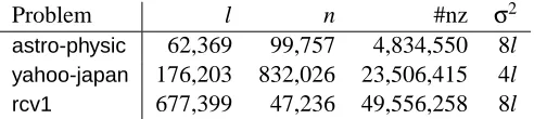
Figure 3: Results on real-valued document data. The first row shows time versus the relative func-tion difference (42). The second and third rows showk∇L(w)kand testing performances along time, respectively. Time is in seconds.
is the common form of regularized logistic regression. We give approximate functions ofIS/CD
methods in Section 7.11.
We compare the same methods: SCGIS,CD,LBFGS, andTRON.GIS is not included because of its slow convergence shown in Section 5.1. Our implementations are based on sources used in Chang et al. (2008).6 We select three data sets considered in Chang et al. (2008). Each instance has been normalized tok¯xik=1. Data statistics andσ2for each problem are in Table 4. We setβ=0.5 andγ=0.01 for the line search procedure (35) in CD. Figure 3 shows the results of the relative function difference to the optimum, the gradientk∇L(w)k, and the testing accuracy.
From Figure 3, the relation between the twoIS/CDmethods is similar to that in Figure 2, where
CDis faster thanSCGIS. However, in contrast to Figure 2, hereTRON/LBFGSmay surpassIS/CD
in an earlier stage. Some preliminary analysis on the cost per iteration seems to indicate thatIS/CD
0 50 100 150 10−3
10−2
10−1
100
101 102
Training Time (s)
Relative function value difference
SCGIS CD CDD
(a) CoNLL2000-Pσ2=10
0 10 20 30 40 50
10−4
10−3
10−2
10−1 100
Training Time (s)
Relative function value difference
SCGIS CD CDD
(b)yahoo-japanσ2=4l
0 50 100 150
10−3 10−2
10−1
100
101
102
Training Time (s)
Relative function value difference
SCGIS CD CDD
(c)CoNLL2000-Pσ2=1
0 10 20 30 40 50
10−4
10−3
10−2
10−1
100
Training Time (s)
Relative function value difference
SCGIS CD CDD
(d)yahoo-japanσ2=0.5l
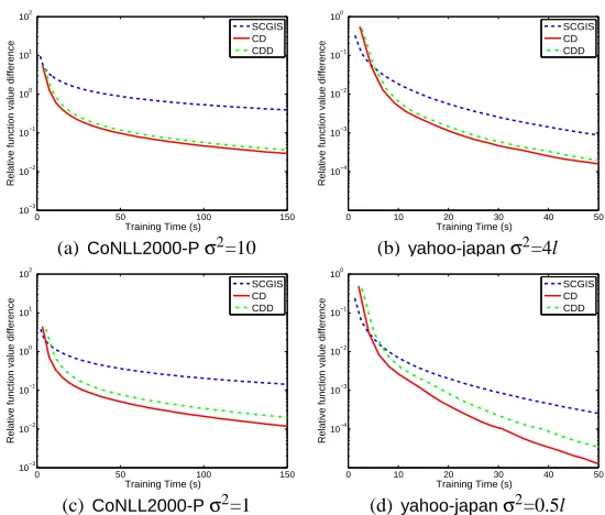
Figure 4: This figure shows the effect of using (38) to do line search. The first and second rows show time versus the relative function difference with differentσ2. CDDindicates theCD
method without using (38). Time is in seconds.
methods are more efficient on 0/1-featured data due to a smaller number of exp operations, but more experiments/data are needed to draw definitive conclusions.
In Figure 3, TRONis only similarly to or moderately better thanLBFGS, but Lin et al. (2008) show thatTRONis much better. The only difference between their setting and ours is that Lin et al. (2008) add one feature to each data instance. That is, they modify ¯xito¯xi
1
, so weights of Maxent become [w
b], where b is called the bias term. It is surprising that this difference affectsLBFGS’ performance that much.
6. Discussion and Conclusions
In (38), we propose a way to speed up the line search procedure of Algorithm 3. Figure 4 shows how effective this trick is by varying the value of σ2. Clearly, the trick is more useful ifσ2 is small. In this situation, the function L(w)is well conditioned (as it is closer to a quadratic function
∑tw2t). Hence (38) more easily holds atλ=1. Then the line search procedure costs only O(1)time. However, a too smallσ2may downgrade the testing accuracy. For example, the final accuracy for
yahoo-japanis 92.75% withσ2=4l, but is 92.31% withσ2=0.5l.
Some work has concluded that approaches likeLBFGSor nonlinear conjugate gradient are better thanISmethods for training Maxent (e.g., Malouf, 2002; Daum´e, 2004). However, experiments in this paper show that comparison results may vary under different circumstances. For example, comparison results can be affected by:
2. TheISmethod being compared. Our experiments indicate thatGISis inferior to many meth-ods, but otherIS/CDmethods likeSCGISorCD(Algorithm 3) are more competitive.
In summary, we create a general framework for iterative scaling and coordinate descent meth-ods for maximum entropy. Based on this framework, we discuss the convergence, computational complexity, and other properties of IS/CD methods. We further develop a new coordinate decent method for Maxent. It is more efficient than existing iterative scaling methods.
7. Proofs and Derivations
We define 1-norm and 2-norm of a vector w∈Rn:
kwk1≡
n
∑
t=1
|wt|, kwk2≡
s
n
∑
t=1
w2t.
The following inequality is useful in our proofs.
kwk2≤ kwk1≤√nkwk2, ∀w∈Rn. (44)
Subsequently we simplifykwk2tokwk. 7.1 Proof of Theorem 1
Due to the regularization term 2σ12wTw, one can prove that the set U defined in (20) is bounded;
see, for example, Theorem 1 of Lin et al. (2008). As∇2L(w)is continuous in the bounded set U , the followingτmaxandτminexist:
τmax≡max
w∈Uλmax(∇
2L(w)) and τ
min≡min
w∈Uλmin(∇
2L(w)), (45)
whereλmax(·)andλmin(·) mean the largest and the smallest eigenvalues of a matrix, respectively. To show thatτmaxandτminare positive, it is sufficient to proveτmin>0. As∇2L(w)is I/σ2plus a positive semi-definite matrix, it is easy to seeτmin≥1/(σ2)>0.
To prove (21), we apply the multi-dimensional Mean-Value Theorem (Apostol, 1974, Theorem 12.9) to∇L(w). If u,v∈Rn, then for any a∈Rn, there is a c=αu+ (1−α)v with 0≤α≤1 such that
aT(∇L(u)−∇L(v)) =aT∇2L(c)(u−v). (46)
Set
a=u−v.
Then for any u,v∈U , there is a point c such that
(u−v)T(∇L(u)−∇L(v)) = (u−v)T∇2L(c)(u−v). (47)
Since U is a convex set from the convexity of L(w), c∈U . With (45) and (47),
Hence
k∇L(u)−∇L(v)k ≥τminku−vk. (48)
By applying (46) again with a=∇L(u)−∇L(v),
k∇L(u)−∇L(v)k2≤k∇L(u)−∇L(v)kk∇2L(c)(u−v)k
≤k∇L(u)−∇L(v)kku−vkτmax.
Therefore,
k∇L(u)−∇L(v)k ≤τmaxku−vk. (49)
Then (21) follows from (48) and (49)
To prove the second property (22), we write the Taylor expansion of L(u):
L(u) =L(v) +∇L(v)T(u−v) +1 2(u−v)
T∇2L(c)(u
−v),
where c∈U . With (45), we have
τmin
2 ku−vk 2
≤L(u)−L(v)−∇L(v)T(u−v)≤τmax
2 ku−vk 2. Sinceτmax≥τmin>0, L satisfies (22) by choosing K=τmax/2.
7.2 Proof of Theorem 2
The following proof is modified from Chang et al. (2008). Since L(w) is convex and w∗ is the unique solution, the optimality condition shows that
∇L(w∗) =0. (50)
From (21) and (50),
k∇L(wk)k ≥τminkwk−w∗k. (51)
With (23) and (51),
kwk+1−wkk ≥ητminkwk−w∗k. (52)
From (24) and (52),
L(wk)−L(wk+1)≥νη2τ2
minkwk−w∗k2. (53)
Combining (22) and (50),
L(wk)−L(w∗)≤Kkwk−w∗k2. (54)
Using (53) and (54),
L(wk)−L(wk+1)≥νη 2τ2
min
K
L(wk)−L(w∗).
This is equivalent to
L(wk)−L(w∗)+L(w∗)−L(wk+1)≥νη 2τ2
min
K
Finally, we have
L(wk+1)−L(w∗)≤
1−νη 2τ2
min
K L(w
k)
−L(w∗). (55)
Let µ≡νη2τ2min/K. As all constants are positive, µ>0. If µ>1, L(wk)>L(w∗) implies that
L(wk+1)<L(w∗), a contradiction to the definition of L(w∗). Thus we have either µ∈(0,1) or
µ=1, which suggests we get the optimum in finite steps.
7.3 Proof of Theorem 3
We prove the result for GIS and IIS first. Let ¯z=arg minzAs(z), where s indicates GIS or IIS
method.7 From the definition of As(z)and its convexity,8
∇As(0) =∇L(wk)and∇As(¯z) =0.9 (56)
Note that∇As(z) is the gradient with respect to z, but∇L(w) is the gradient with respect to w. Since U is bounded, the set{(w,z)|w∈U and w+z∈U}is also bounded. Thus we have that
max
w∈Uz:wmax+z∈Uλmax ∇ 2As(z)
is bounded by a constant K. Hereλmax(·)means the largest eigenvalue of a matrix. To prove (23), we use
kwk+1−wkk=k¯z−0k
≥K1k∇As(¯z)−∇As(0)k= 1
Kk∇A
s(0)
k= 1
Kk∇L(w
k)
k, (57)
where the inequality is from the same derivation for (49) in Theorem 1. The last two equalities follow from (56).
Next, we prove (24). By (56) and the fact that the minimal eigenvalue of∇2As(z)is greater than or equal to 1/(σ2), we have
As(0)≥As(¯z)−∇As(¯z)T¯z+ 1 2σ2¯z
T¯z=As(¯z) + 1 2σ2¯z
T¯z. (58)
From (9) and (58),
L(wk)−L(wk+1) =L(wk)−L(wk+¯z)≥As(0)−As(¯z)≥ 1 2σ2¯z
T¯z= 1 2σ2kw
k+1
−wkk2.
Letν=1/(2σ2)and we obtain (24).
We then prove results for SCGISandCD. For the convenience, we define some notation. A sequential algorithm starts from an initial point w0, and produces a sequence{wk}∞k=0. At each iter-ation, wk+1is constructed by sequentially updating each component of wk. This process generates vectors wk,t ∈Rn, t=1, . . . ,n, such that wk,1=wk, wk,n+1=wk+1, and
wk,t = [wk1+1, . . . ,wtk−+11,wtk, . . . ,wkn]T for t=2, . . . ,n.
7. The existence of ¯z follows from that U is bounded. See the explanation in the beginning of Section 7.1. 8. It is easy to see that all At(zt)in Table 1 are strictly convex.
9. Because∇tL(wk) =ACDt ′(0), we can easily obtain∇As(0) =∇L(wk)by checking Ast′(0) =A
CD
t ′(0), where s isGIS