A Binary-Classification-Based Metric between Time-Series
Distributions and Its Use in Statistical and Learning Problems
Daniil Ryabko [email protected]
J´er´emie Mary [email protected]
SequeL-INRIA/LIFL-CNRS Universit´e de Lille, France 40, avenue de Halley 59650 Villeneuve d’Ascq France
Editor:L´eon Bottou
Abstract
A metric between time-series distributions is proposed that can be evaluated using binary classi-fication methods, which were originally developed to work on i.i.d. data. It is shown how this metric can be used for solving statistical problems that are seemingly unrelated to classification and concern highly dependent time series. Specifically, the problems of time-series clustering, homogeneity testing and the three-sample problem are addressed. Universal consistency of the re-sulting algorithms is proven under most general assumptions. The theoretical results are illustrated with experiments on synthetic and real-world data.
Keywords: time series, reductions, stationary ergodic, clustering, metrics between probability distributions
1. Introduction
Binary classification is one of the most well-understood problems of machine learning and statistics: a wealth of efficient classification algorithms has been developed and applied to a wide range of applications. Perhaps one of the reasons for this is that binary classification is conceptually one of the simplest statistical learning problems. It is thus natural to try and use it as a building block for solving other, more complex, newer or just different problems; in other words, one can try to obtain efficient algorithms for different learning problems by reducing them to binary classification. This approach has been applied to many different problems, starting with multi-class classification, and including regression and ranking (Balcan et al., 2007; Langford et al., 2006), to give just a few examples. However, all of these problems are formulated in terms of independent and identically distributed (i.i.d.) samples. This is also the assumption underlying the theoretical analysis of most of the classification algorithms.
We show how the considered problems can be reduced to binary classification methods, via a new metric between time-series distributions. The results include asymptotically consistent algo-rithms, as well as finite-sample analysis. To establish the consistency of the suggested methods, for clustering and the three-sample problem the only assumption that we make on the data is that the distributions generating the samples are stationary ergodic; this is one of the weakest assumptions used in statistics. For homogeneity testing we have to make some mixing assumptions in order to obtain consistency results (this is indeed unavoidable, as shown by Ryabko, 2010b). Mixing conditions are also used to obtain finite-sample performance guarantees for the first two problems.
The proposed approach is based on a new distance between time-series distributions (that is,
between probability distributions on the space of infinite sequences), which we calltelescope
dis-tance. This distance can be evaluated using binary classification methods, and its finite-sample estimates are shown to be asymptotically consistent. Three main building blocks are used to con-struct the telescope distance. The first one is a distance on finite-dimensional marginal distributions. The distance we use for this is the following well-known metric: dH(P,Q):=suph∈H |EPh−EQh|
whereP,Qare distributions and
H
is a set of functions. This distance can be estimated using binaryclassification methods, and thus can be used to reduce various statistical problems to the classifi-cation problem. This distance was previously applied to such statistical problems as homogeneity testing and change-point estimation (Kifer et al., 2004). However, these applications so far have only concerned i.i.d. data, whereas we want to work with highly-dependent time series. Thus, the second building block are the recent results of Adams and Nobel (2012), that show that
empiri-cal estimates ofdH are consistent (under certain conditions on
H
) for arbitrary stationary ergodicdistributions. This, however, is not enough: evaluatingdH for (stationary ergodic) time-series
dis-tributions means measuring the distance between their finite-dimensional marginals, and not the distributions themselves. Finally, the third step to construct the distance is what we calltelescoping. It consists in summing the distances for all the (infinitely many) finite-dimensional marginals with decreasing weights. The resulting distance can “automatically” select the marginal distribution of the right order: marginals which cannot distinguish between the distributions give distance esti-mates that converge to zero, while marginals whose orders are too high to have converged have very small weights. Thus, the estimate is dominated by the marginals which can distinguish between the time-series distributions, or converges to zero if the distributions are the same. It is worth noting that a similar telescoping trick is used in different problems, most notably, in sequence prediction (Solomonoff, 1978; B. Ryabko, 1988; Ryabko, 2011); it is also used in the distributional distance (Gray, 1988), see Section 8 below.
We show that the resulting distance (telescope distance) indeed can be consistently estimated based on sampling, for arbitrary stationary ergodic distributions. Further, we show how this fact can be used to construct consistent algorithms for the considered problems on time series. Thus we can harness binary classification methods to solve statistical learning problems concerning time series. A remarkable feature of the resulting methods is that the performance guarantees obtained do not depend on the approximation error of the binary classification methods used, they only depend on their estimation error.
Moreover, we analyse some other distances between time-series distributions, the possibility of their use for solving the statistical problems considered, and the relation of these distances to the telescope distance introduced in this work.
problem of binary classification. Experiments on both synthetic and real-world data are provided. The real-world setting concerns brain-computer interface (BCI) data, which is a notoriously chal-lenging application, and on which the presented algorithm demonstrates competitive performance.
A related approach to address the problems considered here, as well as some related problems about stationary ergodic time series, is based on (consistent) empirical estimates of the distributional distance, see Ryabko and Ryabko (2010), Ryabko (2010a), Khaleghi et al. (2012), as well as Gray (1988) about the distributional distance. The empirical distance is based on counting frequencies of bins of decreasing sizes and “telescoping.” This distance is described in some detail in Section 8 below, where we compare it to the telescope distance. Another related approach to time-series analysis involves a different reduction, namely, that to data compression (B. Ryabko, 2009).
1.1 Organisation
Section 2 is preliminary. In Section 3 we introduce and discuss the telescope distance. Section 4 explains how this distance can be calculated using binary classification methods. Sections 5 and 6 are devoted to the three-sample problem and clustering, respectively. In Section 7, under some
mixing conditions, we address the problems of homogeneity testing, clustering with unknownk, and
finite-sample performance guarantees. In Section 8 we take a look at other distances between time-series distributions and their relations to the telescope distance. Section 9 presents experimental evaluation.
2. Notation and Definitions
Let (
X
,F
1) be a measurable space (the domain), and denote (X
k,F
k) and (
X
N,F
) the productprobability space over
X
k and the induced probability space over the one-way infinite sequencestaking values in
X
. Time-series (or process) distributions are probability measures on the space(XN,
F
). We use the abbreviationX1..k for X1, . . . ,Xk. A setH
of functions is called separableif there is a countable set
H
′ of functions such that any function inH
is a pointwise limit of asequence of elements of
H
′.A distributionρis called stationary ifρ(X1..k∈A) =ρ(Xn+1..n+k∈A)for allA∈
F
k,k,n∈N. A stationary distribution is called (stationary) ergodic iflim n→∞
1
ni=1..
∑
n−k+1IXi..i+k∈A=ρ(A) ρ−a.s.for every A∈
F
k, k∈N. (This definition, which is more suited for the purposes of this work, isequivalent to the usual one expressed in terms of invariant sets, see, e.g., Gray, 1988.)
3. A Distance between Time-Series Distributions
We start with a distance between distributions on
X
, and then we extend it to distributions onX
N.For two probability distributionsPandQon(
X
,F
1)and a setH
of measurable functions onX
, onecan define the distance
dH(P,Q):=sup h∈H|
EPh−EQh|. (1)
and Rubinstein, 1957) and Fortet-Mourier (Fortet and Mourier, 1953) metrics. Note that the dis-tance function so defined may not be measurable; however, it is measurable under mild conditions
which we assume whenever necessary. In particular, separability of
H
is a sufficient condition(separability is required in most of the results below).
We are interested in the cases wheredH(P,Q) =0 impliesP=Q. Note that in this casedH is a metric (the rest of the properties are easy to see). For reasons that will become apparent shortly (see
Remark below), we are mainly interested in the sets
H
that consist of indicator functions. In thiscase we can identify each f ∈
H
with the indicator set{x: f(x) =1} ⊂X
and (by a slight abuse of notation) writedH(P,Q):=suph∈H |P(h)−Q(h)|.In this case it is easy to check that the following statement holds true.Lemma 1 dH is a metric on the space of probability distributions over
X
if and only ifH
gener-atesF
1.The property that
H
generatesF
1 is often easy to verify directly. First of all, it trivially holds forthe case where
H
is the set of halfspaces in a EuclideanX
. It is also easy to check that it holds ifH
is the set of halfspaces in the feature space of most commonly used kernels (provided the featurespace is of the same or higher dimension than the input space), such as polynomial and Gaussian kernels.
Based ondH we can construct a distance between time-series probability distributions. For two
time-series distributionsρ1,ρ2 we take thedH betweenk-dimensional marginal distributions ofρ1
andρ2for eachk∈N, and sum them all up with decreasing weights.
Definition 2 (telescope distanceDH) For two time series distributions ρ1 and ρ2 on the space
(
X
N,F
)and a sequence of sets of functionsH= (H
1,H
2, . . .)define thetelescope distance DH(ρ1,ρ2):=∞
∑
k=1 wksup
h∈Hk
|Eρ1h(X1, . . . ,Xk)−Eρ2h(Y1, . . . ,Yk)|, (2)
where wk, k∈Nis a sequence of positive summable real weights (e.g., wk=1/k2or wk=2−k).
Lemma 3 DHis a metric if and only if dHk is a metric for every k∈N.
Proof The statement follows from the fact that two process distributions are the same if and only if all their finite-dimensional marginals coincide.
Definition 4 (empirical telescope distanceDˆ) For a pair of samples X1..nand Y1..mdefine the
em-pirical telescope distanceas
ˆ
DH(X1..n,Y1..m):= min{m,n}
∑
k=1
wk sup h∈Hk
1 n−k+1
n−k+1
∑
i=1
h(Xi..i+k−1)− 1 m−k+1
m−k+1
∑
i=1
h(Yi..i+k−1)
. (3)
Theorem 5 LetH= (
H
k)k∈Nbe a sequence of separable setsH
k of indicator functions (overX
k) of finite VC dimension such thatH
k generatesF
k. Then for every stationary ergodic time series distributionsρX andρY generating samples X1..nand Y1..mwe havelim
n,m→∞DˆH(X1..n,Y1..m) =DH(ρX,ρY)a.s.
Note that ˆDHis a biased estimate ofDH, and, unlike in the i.i.d. case, the bias may depend on the
distributions; however, the bias iso(n).
Remark. The condition that the sets
H
kare sets of indicator function of finite VC dimension comes from the results of Adams and Nobel (2012), who show that for any stationary ergodic distributionρ, under these conditions, suph∈Hk
1 n−k+1∑
n−k+1
i=1 h(Xi..i+k−1)is an asymptotically consistent estimate of suph∈HkEρh(X1, . . . ,Xk). This fact implies thatdHk can be consistently estimated, from which the
theorem is derived.
Proof [of Theorem 5] As established by Adams and Nobel (2012), under the conditions of the theorem we have
lim n→∞hsup
∈Hk
1 n−k+1
n−k+1
∑
i=1
h(Xi..i+k−1) = sup h∈Hk
EρXh(X1, . . . ,Xk)ρX-a.s. (4)
for allk∈N, and likewise forρY. Fix anε>0. We can find aT ∈Nsuch that
∑
k>T
wk≤ε. (5)
Note thatT depends only onε. Moreover, as follows from (4), for eachk=1..T we can find anNk
such that
sup
h∈Hk
1 n−k+1
n−k+1
∑
i=1
h(Xi..i+k−1)−sup h∈Hk
EρXh(X1..k)
≤ε/T. (6)
LetNk:=maxi=1..TNiand define analogouslyMforρY. Thus, forn≥N,m≥Mwe have
ˆ
DH(X1..n,Y1..m)
≤
T
∑
k=1 wk sup
h∈Hk 1 n−k+1
n−k+1
∑
i=1
h(Xi..i+k−1)− 1 m−k+1
m−k+1
∑
i=1
h(Yi..i+k−1)
+ε ≤ T
∑
k=1 wksuph∈Hk ( 1 n−k+1
n−k+1
∑
i=1
h(Xi..i+k−1)−Eρ1h(X1..k)
+|Eρ1h(X1..k)−Eρ2h(Y1..k)|
+
Eρ2h(Y1..k)− 1 m−k+1
m−k+1
∑
i=1
h(Yi..i+k−1)
) +ε
≤3ε+DH(ρX,ρY),
where the first inequality follows from the definition (3) of ˆDHand from (5), and the last inequality
4. CalculatingDˆH Using Binary-Classification Methods
The methods for solving various statistical problems that we suggest are all based on ˆDH. The main
appeal of this approach is that ˆDHcan be calculated using binary classification methods. Here we
explain how to do it.
The definition (3) ofDH involves calculatinglsummands (wherel:=min{n,m}), that is
sup h∈Hk
1 n−k+1
n−k+1
∑
i=1
h(Xi..i+k−1)− 1 m−k+1
m−k+1
∑
i=1
h(Yi..i+k−1)
(7)
for eachk=1..l. Assuming thath∈
H
kare indicator functions, calculating each of the summandsamounts to solving the followingk-dimensional binary classification problem. ConsiderXi..i+k−1, i=1..n−k+1 as class-1 examples andYi..i+k−1,i=1..m−k+1 as class-0 examples. The
supre-mum (7) is attained on h∈
H
k that minimizes the empirical risk, with examples weighted withrespect to the sample size. Indeed, we can define the weighted empirical risk of anyh∈
H
kas1 n−k+1
n−k+1
∑
i=1
(1−h(Xi..i+k−1)) + 1 m−k+1
m−k+1
∑
i=1
h(Yi..i+k−1), (8)
minimising which can be easily seen to be equivalent to (7).
Thus, as long as we have a way to find h∈
H
k that minimizes empirical risk, we have acon-sistent estimate of DH(ρX,ρY), under the mild conditions on H required by Theorem 5. Since
the dimension of the resulting classification problems grows with the length of the sequences, one should prefer methods that work in high dimensions, such as soft-margin SVMs (Cortes and Vapnik, 1995).
A particularly remarkable feature is thatthe choice of
H
kis much easierfor the problems that weconsiderthan in the binary classificationproblem. Specifically, if (for some fixedk) the classifier
that achieves the minimal (Bayes) error for the classification problem is not in
H
k, then obviouslythe error of an empirical risk minimizer will not tend to zero, no matter how much data we have. In contrast, all we need to achieve asymptotically 0 error in estimating ˆD(and therefore, in the learning
problems considered below) is that the sets
H
kgenerateF
kand have a finite VC dimension (for eachk). This is the case already for the set of half-spaces inRk. In other words, theapproximationerror
of the binary classification method (the classification error of the best f in
H
k) is not important.What is important is the estimation error; for asymptotic consistency results it has to go to 0 (hence the requirement on the VC dimension); for non-asymptotic results, it will appear in the error bounds, see Section 7. Thus, we have the following statement.
Claim 1 The error|DH(ρX,ρY)−DˆH(X,Y)|, and thus the error of the algorithms below, can be
much smaller than the error of classification algorithms used to calculate DH(X,Y).
We can conclude that, beyond the requirement that
H
k generateF
k for eachk∈N, the choiceofHk (or, say, of the kernel to use in SVM) is entirely up to the needs and constraints of specific
applications.
Remark (number of summands inDˆH) Finally, we note that while in the definition of the
samples), it can be replaced with anyγl such thatγl→∞, without affecting any asymptotic consis-tency results. In other words, Theorem 5, as well as all the consisconsis-tency statements below, holds true
forlreplaced with any non-decreasing functionγl that tends to infinity withl. A practically viable
choice isγl =logl; in fact, there is no reason to choose faster growingγn since the estimates for
higher-order summands will not have enough data to converge. This is also the value we use in the experiments.
Remark (relation to total variation) An illustrative example1 of the choice of the sets
H
k is the set of indicators of all measurable subsets ofX
k. In this case each summand in (2) is the totalvari-ation distance between thek-dimensional marginal distributions ofρ1andρ2. Take, for simplicity,
k=1; denoting P andQ the corresponding single-dimensional marginals, the distance becomes
supA|P(A)−Q(A)|(cf. (1)). This supremum is reached on the setA∗:={x∈
X
: f(x)≥g(x)},where f andgare densities ofPandQwith respect to some arbitrary measure that dominates both
PandQ(e.g., 1/2(P+Q)). A binary classifier corresponding to a setAdeclaresPifx∈AandQ otherwise. The optimal classification error is infA(1−P(A) +Q(A)) =1−supA(P(A) +Q(A)) = 1−P(A∗) +Q(A∗)(cf. (8)). In general, estimating the total variation distance (and finding the best classifier) is not possible, so using smaller sets
H
kcan be viewed as a regularization of this problem.5. The Three-Sample Problem
We start with a conceptually simple problem known in statistics as the three-sample problem (some-times also called time-series classification). We are given three samples X = (X1, . . . ,Xn), Y =
(Y1, . . . ,Ym)andZ= (Z1, . . . ,Zl). It is known thatX andY were generated by different time-series
distributions, whereasZ was generated by the same distribution as either X orY. It is required
to find out which one is the case. Both distributions are assumed to be stationary ergodic, but no further assumptions are made about them (no independence, mixing or memory assumptions). The three sample-problem for dependent time series has been addressed by Gutman (1989) for Markov processes and by Ryabko and Ryabko (2010) for stationary ergodic time series. The latter work uses an approach based on the distributional distance.
Indeed, to solve this problem it suffices to have consistent estimates of some distance between time series distributions. Thus, we can use the telescope distance. The following statement is a simple corollary of Theorem 5.
Theorem 6 Let the samples X= (X1, . . . ,Xn), Y = (Y1, . . . ,Ym)and Z= (Z1, . . . ,Zl) be generated by stationary ergodic distributions ρX,ρY and ρZ, with ρX 6=ρY and either (i) ρZ =ρX or (ii)
ρZ =ρY. Let the sets
H
k, k∈Nbe separable sets of indicator functions overX
k. Assume that each setH
k, k∈Nhas a finite VC dimension and generatesF
k. A test that declares that (i) is true ifDˆH(Z,X)≤DˆH(Z,Y) and that (ii) is true otherwise, makes only finitely many errors withprobability 1 as n,m,l→∞.
It is straightforward to extend this theorem to more than two classes; in other words, instead ofX
andY one can have an arbitrary number of samples from different stationary ergodic distributions.
A further generalization of this problem is the problem of time-series clustering, considered in the next section.
6. Clustering Time Series
We are givenNtime-series samplesX1= (X11, . . . ,Xn11), . . . ,XN= (X1N, . . . ,XnNN), and it is required to
cluster them intoKgroups, where, in different settings,Kmay be either known or unknown. While
there may be many different approaches to define what should be considered a good clustering, and, thus, what it means to have a consistent clustering algorithm, for the problem of clustering time-series samples there is a natural choice, proposed by Ryabko (2010a): Assume that each of the time-series samplesX1= (X11, . . . ,Xn11), . . . ,XN= (X1N, . . . ,XnNN)was generated by one out ofK different time-series distributionsρ1, . . . ,ρK. These distributions are unknown. Thetarget clustering is defined according to whether the samples were generated by the same or different distributions: the samples belong to the same cluster if and only if they were generated by the same distribution.
A clustering algorithm is calledasymptotically consistentif with probability 1 from some non it
outputs the target clustering, wherenis the length of the shortest samplen:=mini=1..Nni≥n′. Again, to solve this problem it is enough to have a metric between time-series distributions that can be consistently estimated. Our approach here is based on the telescope distance, and thus we use ˆD.
The clustering problem is relatively simple if the target clustering has what is called thestrict
separation property (Balcan et al., 2008): every two points in the same target cluster are closer to each other than to any point from a different target cluster. The following statement is an easy corollary of Theorem 5.
Theorem 7 Let the sets
H
k, k∈Nbe separable sets of indicator functions overX
k. Assume that each setH
k, k∈N has a finite VC dimension and generatesF
k. If the distributions ρ1, . . . ,ρK generating the samples X1= (X11, . . . ,Xn11), . . . ,XN= (XN1, . . . ,XnNN)are stationary ergodic, then with
probability 1 from some n:=mini=1..Nnion the target clustering has the strict separation property with respect toDˆH.
With the strict separation property at hand, if the number of clusters K is known, it is easy to
find asymptotically consistent algorithms. Here we give some simple examples, but the theorem below can be extended to many other distance-based clustering algorithms.
The average linkagealgorithm works as follows. The distance between clusters is defined as the average distance between points in these clusters. First, put each point into a separate cluster.
Then, merge the two closest clusters; repeat the last step until the total number of clusters is K.
The farthest pointclustering works as follows. Assignc1:=X1 to the first cluster. Fori=2..K, find the pointXj, j∈ {1..N}that maximizes the distance mint=1..iDˆH(Xj,ct)(to the points already
assigned to clusters) and assignci:=Xj to the clusteri. Then assign each of the remaining points
to the nearest cluster. The following statement is a corollary of Theorem 7.
Theorem 8 Under the conditions of Theorem 7, average linkage and farthest point clusterings are asymptotically consistent, provided the correct number of clusters K is given to the algorithm.
Note that we do not require the samples to be independent; the joint distributions of the samples may be completely arbitrary, as long as the marginal distribution of each sample is stationary ergodic. These results can be extended to the online setting in the spirit of Khaleghi et al. (2012).
7. Speed of Convergence
The results established so far are asymptotic out of necessity: they are established under the as-sumption that the distributions involved are stationary ergodic, which is too general to allow for any meaningful finite-time performance guarantees. While it is interesting to be able to establish consis-tency results under such general assumptions, it is also interesting to see what results can be obtained under stronger assumptions. Moreover, since it is usually not known in advance whether the data
at hand satisfies given assumptions or not, it appears important to have methods that have both
asymptotic consistency in the general setting and finite-time performance guarantees under stronger assumptions. It turns out that this is possible: for the methods based on ˆDone can establish both the asymptotic performance guarantees for all stationary ergodic distributions and finite-sample perfor-mance guarantees under stronger assumptions, namely the uniform mixing conditions introduced below.
Another reason to consider stronger assumptions on the distributions generating the data is that some statistical problems, such as homogeneity testing or clustering when the number of clusters is unknown, are provably impossible to solve under the only assumption of stationary ergodic distri-butions, as shown by Ryabko (2010b).
Thus, in this section we analyse the speed of convergence of ˆDunder certain mixing conditions,
and use it to construct solutions for the problems of homogeneity and clustering with an unknown number of clusters, as well as to establish finite-time performance guarantees for the methods pre-sented in the previous sections.
A stationary distribution on the space of one-way infinite sequences (
X
N,F
) can be uniquelyextended to a stationary distribution on the space of two-way infinite sequences (
X
Z,F
Z) of theform. . . ,X−1,X0,X1, . . ..
Definition 9 (β-mixing coefficients) For a process distributionρdefine the mixing coefficients
β(ρ,k):= sup A∈σ(X−∞..0),
B∈σ(Xk..∞)
|ρ(A∩B)−ρ(A)ρ(B)|
whereσ(..)denotes the sigma-algebra of the random variables in brackets.
Whenβ(ρ,k)→0 the processρis called uniformlyβ-mixing (with coefficientsβ(ρ,k)); this
con-dition is much stronger than ergodicity, but is much weaker than the i.i.d. assumption. For more information on mixing see, for example, Bosq (1996).
7.1 Speed of Convergence ofDˆ
Assume that a sampleX1..n is generated by a distributionρthat is uniformlyβ-mixing with
coeffi-cientsβ(ρ,k). Assume further that
H
k is a set of indicator functions with a finite VC dimensiondk,for eachk∈N.
Since in this section we are after finite-time bounds, we fix a concrete choice of the weightswk
in the definition of ˆD(Definition 2),
The general tool that we use to obtain performance guarantees in this section is the following bound that can be obtained from the results of Karandikar and Vidyasagar (2002).
qn(ρ,
H
k,ε):=ρ sup h∈Hk1 n−k+1
n−k+1
∑
i=1
h(Xi..i+k−1)−Eρh(X1..k)
>ε !
≤nβ(ρ,tn−k) +8tndk+1e−lnε
2/8
, (10)
wheretn are any integers in 1..nandln=n/tn. The parameterstn should be set according to the
values ofβin order to optimize the bound.
One can use similar bounds for classes of finite Pollard dimension (Pollard, 1984) or more general bounds expressed in terms of covering numbers, such as those given by Karandikar and Vidyasagar (2002). Here we consider classes of finite VC dimension only for the ease of the expo-sition and for the sake of continuity with the previous section (where it was necessary).
Furthermore, for the rest of this section we assume geometric β-mixing distributions, that is,
β(ρ,t)≤γt for someγ<1. Lettingl
n=tn=√nthe bound (10) becomes
qn(ρ,
H
k,ε)≤nγ √n−k+8n(dk+1)/2e−√nε2/8. (11) Lemma 10 Let two samples X1..n and Y1..m be generated by stationary distributions ρX and ρY whose β-mixing coefficients satisfy β(ρ.,t)≤γt for some γ<1. Let
H
k, k∈N be some sets of indicator functions on
X
kwhose VC dimension dk is finite and non-decreasing with k. Then
P(|DˆH(X1..n,Y1..m)−DH(ρX,ρY)|>ε)≤2∆(ε/4,n′) (12) where n′:=min{n,m}, the probability is with respect toρX×ρY and
∆(ε,n):=−logε(nγ√n+log(ε)+8n(d−logε+1)/2e−√nε2/8). (13)
ProofFrom (9) we have∑∞k=−logε/2wk<ε/2. Using this and the definitions 2 and 4 ofDHand ˆDH
we obtain
P(|DˆH(X1..n
1,Y1..n2)−DH(ρX,ρY)|>ε)≤
−log(ε/2)
∑
k=1
(qn(ρX,
H
k,ε/4) +qn(ρY,H
k,ε/4)),which, together with (11), implies the statement.
7.2 Homogeneity Testing
Given two samplesX1..n andY1..m generated by distributionsρX andρY respectively, the problem
of homogeneity testing (or the two-sample problem) consists in deciding whetherρX =ρY. A test
is called (asymptotically) consistent if its probability of error goes to zero asn′:=min{m,n}goes to infinity. As mentioned above, in general, for stationary ergodic time series distributions there is no asymptotically consistent test for homogeneity (Ryabko, 2010b) (even for binary-valued time series); thus, stronger assumptions are in order.
processes as well. We do not attempt to survey this literature here. Our contribution to this line of research is to show that this problem can be reduced (via the telescope distance) to binary classifi-cation, in the case of strongly dependent processes satisfying some mixing conditions.
It is easy to see that under the mixing conditions of Lemma 10 a consistent test for homogeneity exists, and finite-sample performance guarantees can be obtained. It is enough to find a sequence
εn→0 such that∆(εn,n)→0 (see (13)). Then the test can be constructed as follows: say that the
two sequencesX1..nandY1..mwere generated by the same distribution if ˆDH(X1..n,Y1..m)<εmin{n,m}; otherwise say that they were generated by different distributions.
Theorem 11 Under the conditions of Lemma 10 the probability of Type I error (the distributions are the same but the test says they are different) of the described test is upper-bounded by2∆(ε/4,n′). The probability of Type II error (the distributions are different but the test says they are the same) is upper-bounded by2∆((δ−ε)/4,n′)whereδ:=DH(ρX,ρY).
Proof The statement is an immediate consequence of Lemma 10. Indeed, for the Type I error, the two sequences are generated by the same distribution, so the probability of error of the test is given by (12) withDH(ρX,ρY) =0. The probability of Type II error is given byP(DH(ρX,ρY)−
ˆ
DH(X1..n1,Y1..n2)>δ−ε), which is upper-bounded by 2∆((δ−ε))/4,n′)as follows from (12).
The optimal choice of εn may depend on the speed at which dk (the VC dimension of
H
k)increases; however, for most natural cases (recall that
H
k are also parameters of the algorithm) thisgrowth is polynomial, so the main term to control ise−√nε2/8 .
For example, if
H
k is the set of halfspaces inX
k =Rk then dk =k+1 and one can chooseεn:=n−1/8. The resulting probability of Type I error decreases as exp(−n1/4).
7.3 Clustering with a Known or Unknown Number of Clusters
If the distributions generating the samples satisfy certain mixing conditions, then we can augment Theorems 7 and 8 with finite-sample performance guarantees.
Theorem 12 Let the distributionsρ1, . . . ,ρkgenerating the samples X1= (X11, . . . ,Xn11), . . . ,X
N=
(X1N, . . . ,XnNN) satisfy the conditions of Lemma 10. Let n := mini=1..Nni and δ := mini,j=1..N,i6=jDH(ρi,ρj). Then with probability at least1−N(N−1)∆(δ/12,n′) the target clus-tering of the samples has the strict separation property. In this case single linkage and farthest point algorithms output the target clustering.
Proof Note that a sufficient condition for the strict separation property to hold is that for every pair i,jof samples generated by the same distribution we have ˆDH(Xi,Xj)≤δ/3, and for every pairi,j
of samples generated by different distributions we have ˆDH(Xi,Xj)≥2δ/3. Using Lemma 10, the
probability of such an even (for each pair) is upper-bounded by 2∆(δ/12,n′), which, multiplied by
the total numberN(N−1)/2 of pairs gives the statement. The second statement is obvious.
As with homogeneity testing, while in the general case of stationary ergodic distributions it is
impossible to have a consistent clustering algorithm when the number of clustersk is unknown,
mostεn-far from each other, where the thresholdεnis selected the same way as for homogeneity
testing:εn→0 and∆(εn,n)→0. The optimal choice of this parameter depends on the choice of
H
kthrough the speed of growth of the VC dimensiondk of these sets.
Theorem 13 Given N samples generated by k different stationary distributions ρi, i=1..k (un-known k) all satisfying the conditions of Lemma 10, the probability of error (misclustering at least one sample) of the described algorithm is upper-bounded by
N(N−1)max{∆(ε/4,n′),∆((δ−ε)/4,n′)}
where δ:=mini,j=1..k,i6=jDH(ρi,ρj) and n=mini=1..Nni, with ni, i=1..N being lengths of the samples.
Proof The statement follows from Theorem 11.
8. Other Metrics for Time-Series Distributions
The previous sections introduce a new metric on the space of time-series distributions, and use its empirical estimates to solve several learning problems. In this section we attempt to put the telescope distance into a more general context, and take a broader look at metrics between time-series distributions.
Introduce the notationµk for thek-dimensional marginal distribution of a time-series
distribu-tionµ.
8.1 sumDistances
Observe that the telescope distanceDHhas the form
D(µ,ν) =
∑
k∈N
wkdk(µk,νk), (14)
wherewkare summable positive real weights.
It is easy to see that distances of this form can be consistently estimated, as long as dk can be
consistently estimated for eachk∈N; this is formalized in the following statement.
Proposition 14 (estimating sum-based distances) Let
C
be a set of distributions overX
N. Let dk,k∈Nbe a series of distances on the spaces of distributions overX
k, such that dk(µk,νk)≤a∈R for all µ,ν∈C
and such that there exists a seriesdˆk(X1..n,Y1..n),k∈Nof their consistent estimates: for each µ,ν∈C
we havelimn→∞dˆk(X1..n,Y1..n) =dk(µk,νk)a.s., whenever µ,ν∈C
are chosen to generate the sequences. Then the distance D given by (14) can be consistently estimated using the estimate∑k∈Nwkdˆk(X1..n,Y1..n).Proof The proof is an easy generalization of the proof of Theorem 5, with the condition on ˆdkused instead of (4).
Clearly, DH is an example of a distance in the form (14), and it satisfies the conditions of the
Another example of a distance in the form (14) is given by the so-called distributional distance (Gray, 1988; Shields, 1996), whose definition is given below. Empirical estimates of this distance are asymptotically consistent for stationary ergodic time series, and thus can be used (Ryabko and Ryabko, 2010; Ryabko, 2010a; Khaleghi et al., 2012; Khaleghi and Ryabko, 2012; Ryabko, 2012) to solve various statistical problems, including those considered above.
To define the distributional distance, let, for each k,l∈N, the set Bk,l be some partition of the set
X
k, such that the setBk =∪l∈NBk,l generates
F
k. Let alsoB
=∪∞k=1Bk. Note that the set{B×
X
N:B∈Bk,l,k,l∈N}generatesF
.Definition 15 (distributional distance) The distributional distance is defined for a pair of pro-cessesρ1,ρ2as follows
Ddd(ρ1,ρ2):=
∞
∑
m,l=1
wmwl
∑
B∈Bm,l|ρ1(B)−ρ2(B)|, (15)
where wk,k∈Nis a summable sequence of positive real weights (e.g., wj=2−j).
Remark. A more general definition, which is not specific to time-series distributions, is to take any sequenceBj∈
F
1, j∈Nof events that generate the sigma-algebraF
of a probability space(X
,F
), and then defineD′dd(ρ1,ρ2):=
∞
∑
j=1
wj|ρ1(Bj)−ρ2(Bj)|; (16) see Gray (1988) for a general treatment. The latter definition is sometimes more convenient for theoretical analysis (Ryabko, 2012), while the distance (15), which makes explicit the marginal
distributions on
X
m, m∈N and the levell of discretisationBm,l of each setX
m, is more suitedfor time-series, and, specifically, for implementing algorithms, see Ryabko and Ryabko (2010), Khaleghi et al. (2012) and Khaleghi and Ryabko (2012).
In general, it is perhaps impossible to tell which distance, specifically, DH orDdd, should be
preferred for which problem. Conceptually, one of the advantages of the telescope distanceDH is
that one can use different setsH—the choice that makes it adaptable to applications. Another is that
one can reuse readily available classification methods for calculating its empirical estimates. One formal way to compare different metrics is to compare the resulting topologies. This is done in the end of this section.
8.2 supDistances
A different way to construct a distance between time-series distributions based on their finite-dimensional marginals is to use the supremum instead of summation in (14):
d(µ,ν) =sup k∈N
dk(µk,νk). (17)
Some commonly used metrics are defined in the form (17) or have natural interpretations in this form, as the following two examples show.
It is easy to see thatDtv(µ,ν) =supk∈NsupA∈Fk|µ(A)−ν(A)|, so that the total variation distance has
the form (17).
However, the total variation distance is not very useful for time-series distributions for the fol-lowing two reasons. First of all, for stationary ergodic distributions it is degenerate:Dtv(µ,ν) =1 if and only ifµ6=ν. This follows from the fact that any two different stationary ergodic distributions are singular. Such a distance could still be useful as a formalization of the problem of homogeneity testing. However, the problem of homogeneity testing is impossible to solve based on sampling for
stationary ergodic distributions (and even for a smaller family ofBprocesses, see below) (Ryabko,
2010b), so the use of this distance remains limited to more restrictive classes of distributions. This hints at an intrinsic problem with distances defined in the form (17). The problem is in the
difficulties to estimate such metrics based on sampling. At each time steptwe observe only a sample
of finite length, saynt, and based on this we want to estimate a quantity that involvesk-dimensional marginals for allk, including those withk>nt. Considering a growing (witht) number of marginals for the estimate may be a route to take, but this turns out to be difficult to analyse, especially if no rates of convergence can be established for the set of time-series distributions at hand. This problem
is highlighted by the example of the so-called ¯d distance, whose definition follows.
Definition 17 (d¯distance) Assume some distanceδover
X
is given. For two time-series distribu-tions µ andνdefine¯
d(µ,ν):=sup k∈N 1 kpinf∈P
k
∑
i=1
Epδ(xi,yi),
where P is the set of all distributions over
X
k×X
k generating a pair of sequences x1..k,y1..kwhose marginal distributions are µk andνkcorrespondingly.
A process is called a B-process (or a Bernoulli process) if it is in the ¯d-closure of the set of all
aperiodic stationary ergodick-step Markov processes, wherek∈N. For more information on ¯
d-distance and B-processes see Gray (1988) and Shields (1996). The set ofB-processes is a strict
subset of the set of all stationary ergodic time-series distributions. It turns out that ¯d distance is impossible to estimate for the latter, while it can be estimated for the former (Ornstein and Weiss, 1990).
Theorem 18 (Ornstein and Weiss, 1990) There exists an estimator dˆ(X1..n,Y1..n) such that, if X1..n,Y1..nare generated by B-processes µ andνthendˆ(X1..n,Y1..n)→d¯(µ,ν)a.s. However, for any estimator dˆ(X1..n,Y1..n) there is a pair of stationary ergodic processes µ and ν such that lim supn→∞|dˆ(X1..n,Y1..n)−d¯(µ,ν)|>1/2.
8.3 Comparison with the Distributional Distance
In this section we show that the telescope distance is stronger than the distributional distance in the topological sense. Since in fact both the telescope distance and the distributional distance are
families of distances (the telescope distance depends on the sequenceH), we will fix a simple natural
Thus, for the purpose of this section, let us fix
X
=Rand letHk0be the set of halfspaces inX
k. DenoteH0:= (H
0k :k∈N). Clearly, these
H
ksatisfy all the conditions of the theorems of Sections 5 and 6.For the distributional distance (Definition 15), setBk,l to be the partition of the set
X
k into k-dimensional cubes with volumehkl = (1/l)k. DenoteD0dd the distributional distanceDddwith this set of parameters.
Definition 19 A metric d1is said to bestrongerthan a metric d2 if any sequence that converges in d1also converges in d2. If, in addition, d2is not stronger than d1, then d1is calledstrictly stronger.
Note that for the distributional distance, if we use the same setsBk to generate the sigma algebras
X
kthen the distance defined by (15) is stronger than the distance defined by (16).Theorem 20 DH0 is strictly stronger than D0dd.
Proof Fix anyε>0 and find aT ∈Nsuch that∑m,l>Twmwl<ε. Letρi,i∈Nbe a sequence of
process measures that converges inDH0. LetAk be the set of all complements to
X
k of cubes withsides of lengths, for alls∈N. Note that any cubeBinBk, as well as any setAinAk, can be obtained
by intersecting 2khalfspaces. Therefore, we have
sup B∈Bk∪Ak|
ρi(B)−ρj(B)| ≤2kdHk(ρi,ρj)≤2kw
−1
k DH0(ρi,ρj), (18)
where the second inequality follows from the definition ofDH0. Observe that for eachi∈None can
find a setAi∈Aksuch thatρi(Ai)<ε/2. From this, (18) and the fact that the sequenceρiconverges inDH0, we conclude that there is a setA∈Aksuch that
ρi(A)<ε
for alli≥ jk. For allk,l∈None can findMk,l ∈Nsuch that the complement ofA(which is a cube in
X
k) is contained in the union ofMk,l cubes fromBk,l. LetM:=maxk,l≤TMk,l andJ:=maxi≤T ji. Using (18) and the definition of the partitionsBk,lwe can derive
∑
B∈Bk,l,B*A k
|ρi(B)−ρj(B)| ≤2MTw−T1DH0(ρi,ρj)
for anyi,j≥J and allk,l≤T. IncreasingJ if necessary to have 2MTw−T1DH0(ρi,ρj)<ε for all i,j≥J, we obtain
D0dd(ρi,ρj)≤ T
∑
m,l=1
wmwl
∑
B∈Bm,l,B*Am
|ρi(B)−ρj(B)|+2ε≤3ε
for alli,j>J, which means that the sequenceρi,i∈Nconverges inD0dd. Thus,DH0 is stronger than D0dd.
It remains to show that D0dd is not stronger thanDH0. To see this, consider the following
0 200 400 600 800 1000 1200
0
.0
0
.1
0
.2
0
.3
0
.4
Time of observation
Erro
r
ra
te
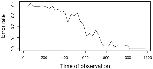
Figure 1: Error of two-class clustering using TSSVM; 10 time series in each target cluster, averaged
over 20 runs.
9. Experimental Evaluation
For experimental evaluation we chose the problem of time-series clustering. The average-linkage clustering is used, with the telescope distance between samples calculated using an SVM, as de-scribed in Section 4. In all experiments, SVM is used with radial basis kernel, with default
parame-ters of libsvm (Chang and Lin, 2011). The parameparame-terswk in the definition of the telescope distance
(Definition 2) are set towk:=k−2.
9.1 Synthetic Data
For the artificial setting we chose highly-dependent time-series distributions which have the same single-dimensional marginals and which cannot be well approximated by finite- or countable-state models. Variants of this family of distributions are standard examples in ergodic theory and dy-namical systems (see, for example, Billingsley, 1965; Gray, 1988; Shields, 1996). The distributions
ρ(α),α∈(0,1), are constructed as follows. Selectr0∈[0,1]uniformly at random; then, for each i=1..nobtainri by shiftingri−1byαto the right, and removing the integer part. The time series
(X1,X2, . . .)is then obtained fromri by drawing a point from a distribution law
N
1ifri<0.5 andfrom
N
2otherwise.N
1is a 3-dimensional Gaussian with mean of 0 and covariance matrix Id×1/4.N
2is the same but with mean 1. Ifαis irrational2then the distributionρ(α)is stationary ergodic,but does not belong to any simpler natural distribution family; in particular, it is not aB-processes
(Shields, 1996). The single-dimensional marginal is the same for all values of α. The latter two
properties make all parametric and most non-parametric methods inapplicable to this problem. In our experiments, we use two process distributionsρ(αi),i∈ {1,2}, withα1=0.31..., α2=
0.35...,. The dependence of error rate on the length of time series is shown on Figure 1. One
clustering experiment on sequences of length 1000 takes about 5 min. on a standard laptop.
9.2 Real Data
To demonstrate the applicability of the proposed methods to realistic scenarios, we chose the brain-computer interface data from BCI competition III (Mill´an, 2004). The data set consists of (pre-processed) BCI recordings of mental imagery: a person is thinking about one of three subjects
s1 s2 s3
TSSVM 84% 81% 61%
DTW 46% 41% 36%
KCpA 79% 74% 61%
SVM 76% 69% 60%
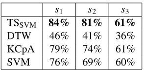
Table 1: Clustering accuracy in the BCI data set. 3 subjects (columns), 4 methods (rows). Our
method is TSSVM.
(left foot, right foot, a random letter). Originally, each time series consisted of several consecutive sequences of different classes, and the problem was supervised: three time series for training and one for testing. We split each of the original time series into classes, and then used our clustering algorithm in a completely unsupervised setting. The original problem is 96-dimensional, but we used only the first 3 dimensions (using all 96 gives worse performance). The typical sequence length is 300. The performance is reported in Table 1, labelled TSSVM. All the computation for this experiment takes approximately 6 minutes on a standard laptop.
The following methods were used for comparison. First, we used dynamic time wrapping (DTW) (Sakoe and Chiba, 1978) which is a popular base-line approach for time-series clustering. The other two methods in Table 1 are from the paper of Harchaoui et al. (2008). The comparison is not fully relevant, since the results of Harchaoui et al. (2008) are for different settings; the method KCpA was used in change-point estimation method (a different but also unsupervised setting), and SVM was used in a supervised setting. The latter is of particular interest since the classification method we used in the telescope distance is also SVM, but our setting is unsupervised (cluster-ing). On this data set the telescope distance demonstrates better performance than the comparison methods, which indicates that it can be useful in real-world scenarios.
10. Outlook
Acknowledgments
This work is an extended version of the NIPS’12 paper (Ryabko and Mary, 2012). The authors are grateful to the anonymous reviewers for the numerous constructive comments that helped us to improve the paper. This research was partially supported by the French Ministry of Higher Education and Research, Nord-Pas-de-Calais Regional Council and FEDER through CPER 2007-2013, ANR project Lampada (ANR-09-EMER-007) and by the European Community’s Seventh Framework Programme (FP7/2007-2013) under grant agreement 231495 (project CompLACS).
References
T. M. Adams and A. B. Nobel. Uniform approximation of Vapnik-Chervonenkis classes.Bernoulli,
18(4):1310–1319, 2012.
M.-F. Balcan, N. Bansal, A. Beygelzimer, D. Coppersmith, J. Langford, and G. Sorkin. Robust
re-ductions from ranking to classification. In Nader Bshouty and Claudio Gentile, editors,Learning
Theory, volume 4539 ofLecture Notes in Computer Science, pages 604–619. 2007.
M.-F. Balcan, A. Blum, and S. Vempala. A discriminative framework for clustering via similarity
functions. InProceedings of the 40th Annual ACM Symposium on Theory of Computing, pages
671–680. ACM, 2008.
P. Billingsley. Ergodic Theory and Information. Wiley, New York, 1965.
D. Bosq. Nonparametric Statistics for Stochastic Processes. Estimation and Prediction. Springer,
1996.
Ch.-Ch. Chang and Ch.-J. Lin. LIBSVM: A library for support vector machines.ACM Transactions
on Intelligent Systems and Technology, 2:27:1–27:27, 2011. Software available athttp://www. csie.ntu.edu.tw/˜cjlin/libsvm.
C. Cortes and V. Vapnik. Support-vector networks. Machine Learning, 20(3):273–297, 1995.
R. Fortet and E. Mourier. Convergence de la r´epartition empirique vers la r´epartition th´eoretique. Ann. Sci. Ec. Norm. Super., III. Ser, 70(3):267–285, 1953.
R. Gray. Probability, Random Processes, and Ergodic Properties. Springer Verlag, 1988.
M. Gutman. Asymptotically optimal classification for multiple tests with empirically observed
statistics. IEEE Transactions on Information Theory, 35(2):402–408, 1989.
Z. Harchaoui, F. Bach, and E. Moulines. Kernel change-point analysis. In Advances in Neural
Information Processing Systems 21, pages 609–616, 2008.
L. V. Kantorovich and G. S. Rubinstein. On a function space in certain extremal problems. Dokl.
Akad. Nauk USSR, 115(6):1058–1061, 1957.
R.L. Karandikar and M. Vidyasagar. Rates of uniform convergence of empirical means with mixing
A. Khaleghi, D. Ryabko, J. Mary, and P. Preux. Online clustering of processes. InAISTATS, JMLR W&CP 22, pages 601–609, 2012.
A. Khaleghi and D. Ryabko. Locating changes in highly dependent data with unknown number of change points. In P. Bartlett, F.C.N. Pereira, C.J.C. Burges, L. Bottou, and K.Q. Weinberger,
editors,Advances in Neural Information Processing Systems 25, pages 3095–3103. 2012.
A. Khaleghi and D. Ryabko. Nonparametric multiple change point estimation in highly
depen-dent time series. In Proc. 24th International Conf. on Algorithmic Learning Theory (ALT’13),
Singapre, 2013. Springer.
D. Kifer, Sh. Ben-David, and J. Gehrke. Detecting change in data streams. InProc. the Thirtieth
International Conference on Very Large Data Bases - Volume 30, VLDB’04, pages 180–191, 2004.
A.N. Kolmogorov. Sulla determinazione empirica di una legge di distribuzione.G. Inst. Ital. Attuari,
pages 83–91, 1933.
J. Langford, R. Oliveira, and B. Zadrozny. Predicting conditional quantiles via reduction to
classi-fication. InProc. of the 22th Conference on Uncertainty in Artificial Intelligence (UAI), 2006.
J. del R. Mill´an. On the need for on-line learning in brain-computer interfaces. InProc. of the Int.
Joint Conf. on Neural Networks, 2004.
D.S. Ornstein and B. Weiss. How sampling reveals a process.Annals of Probability, 18(3):905–930,
1990.
D. Pollard. Convergence of Stochastic Processes. Springer, 1984.
B. Ryabko. Prediction of random sequences and universal coding. Problems of Information
Trans-mission, 24:87–96, 1988.
B. Ryabko. Compression-based methods for nonparametric prediction and estimation of some
char-acteristics of time series. IEEE Transactions on Information Theory, 55:4309–4315, 2009.
D. Ryabko. Clustering processes. InProc. the 27th International Conference on Machine Learning
(ICML 2010), pages 919–926, Haifa, Israel, 2010a.
D. Ryabko. Discrimination between B-processes is impossible. Journal of Theoretical Probability,
23(2):565–575, 2010b.
D. Ryabko. On the relation between realizable and non-realizable cases of the sequence prediction
problem. Journal of Machine Learning Research, 12:2161–2180, 2011.
D. Ryabko. Testing composite hypotheses about discrete ergodic processes. Test, 21(2):317–329,
2012.
D. Ryabko and B. Ryabko. Nonparametric statistical inference for ergodic processes. IEEE
D. Ryabko and J. Mary. Reducing statistical time-series problems to binary classification. In
P. Bartlett, F.C.N. Pereira, C.J.C. Burges, L. Bottou, and K.Q. Weinberger, editors, Advances
in Neural Information Processing Systems 25, pages 2069–2077. 2012.
H. Sakoe and S. Chiba. Dynamic programming algorithm optimization for spoken word recognition. IEEE Transactions on Acoustics, Speech and Signal Processing, 26(1):43–49, 1978.
P. Shields. The Ergodic Theory of Discrete Sample Paths. AMS Bookstore, 1996.
R. J. Solomonoff. Complexity-based induction systems: comparisons and convergence theorems. IEEE Trans. Information Theory, IT-24:422–432, 1978.
V. M. Zolotarev. Probability metrics. Theory of Probability and Its Applications., 28(2):264–287,