Node-Based Learning of Multiple Gaussian Graphical Models

Node-Based Learning of

Multiple Gaussian Graphical Models

Karthik Mohan [email protected]

Palma London [email protected]

Maryam Fazel [email protected]

Department of Electrical Engineering University of Washington

Seattle WA, 98195

Daniela Witten [email protected]

Department of Biostatistics University of Washington Seattle WA, 98195

Su-In Lee [email protected]

Departments of Computer Science and Engineering, Genome Sciences University of Washington

Seattle WA, 98195

Editor:Saharon Rosset

Abstract

We consider the problem of estimating high-dimensional Gaussian graphical models cor-responding to a single set of variables under several distinct conditions. This problem is motivated by the task of recovering transcriptional regulatory networks on the basis of gene expression data containing heterogeneous samples, such as different disease states, multiple species, or different developmental stages. We assume that most aspects of the conditional dependence networks are shared, but that there are some structured differences between them. Rather than assuming that similarities and differences between networks are driven by individual edges, we take anode-based approach, which in many cases provides a more intuitive interpretation of the network differences. We consider estimation under two dis-tinct assumptions: (1) differences between the K networks are due to individual nodes that areperturbed across conditions, or (2) similarities among the K networks are due to the presence ofcommon hub nodes that are shared across allK networks. Using a row-column overlap norm penalty function, we formulate two convex optimization problems that correspond to these two assumptions. We solve these problems using an alternating direction method of multipliers algorithm, and we derive a set of necessary and sufficient conditions that allows us to decompose the problem into independent subproblems so that our algorithm can be scaled to high-dimensional settings. Our proposal is illustrated on synthetic data, a webpage data set, and a brain cancer gene expression data set.

1. Introduction

Graphical models encode the conditional dependence relationships among a set ofpvariables (Lauritzen, 1996). They are a tool of growing importance in a number of fields, including finance, biology, and computer vision. A graphical model is often referred to as a conditional

dependence network, or simply as a network. Motivated by network terminology, we can

refer to thepvariables in a graphical model asnodes. If a pair of variables are conditionally

dependent, then there is an edge between the corresponding pair of nodes; otherwise, no

edge is present.

Suppose that we havenobservations that are independently drawn from a multivariate

normal distribution with covariance matrix Σ. Then the corresponding Gaussian graphical

model (GGM) that describes the conditional dependence relationships among the variables is encoded by the sparsity pattern of the inverse covariance matrix, Σ−1 (see, e.g., Mardia et al., 1979; Lauritzen, 1996). That is, the jth and j0th variables are conditionally inde-pendent if and only if (Σ−1₎

jj0 = 0. Unfortunately, when p > n, obtaining an accurate

estimate of Σ−1 is challenging. In such a scenario, we can use prior information—such as

the knowledge that many of the pairs of variables are conditionally independent—in order

to more accurately estimate Σ−1 (see, e.g., Yuan and Lin, 2007a; Friedman et al., 2007;

Banerjee et al., 2008).

In this paper, we consider the task of estimatingK GGMs on a single set ofp variables

under the assumption that the GGMs are similar, with certain structured differences. As a motivating example, suppose that we have access to gene expression measurements for

n1 lung cancer samples and n2 normal lung samples, and that we would like to estimate

the gene regulatory networks underlying the normal and cancer lung tissue. We can model each of these regulatory networks using a GGM. We have two obvious options.

1. We can estimate a single network on the basis of alln1+n2 tissue samples. But this

approach overlooks fundamental differences between the true lung cancer and normal gene regulatory networks.

2. We can estimate separate networks based on the n1 cancer and n2 normal samples.

However, this approach fails to exploit substantial commonality of the two networks, such as lung-specific pathways.

In order to effectively make use of the available data, we need a principled approach for jointly estimating the two networks in such a way that the two estimates are encouraged to be quite similar to each other, while allowing for certain structured differences. In fact, these differences may be of scientific interest.

Another example of estimating multiple GGMs arises in the analysis of the conditional

dependence relationships among p stocks at two distinct points in time. We might be

interested in detecting stocks that have differential connectivity with all other stocks across the two time points, as these likely correspond to companies that have undergone significant changes. Yet another example occurs in the field of neuroscience, in which it is of interest to learn how the connectivity of neurons changes over time.

Past work on joint estimation of multiple GGMs has assumed that individual edges

this paper, we instead take anode-based approach: we seek to estimateK GGMs under the assumption that similarities and differences between networks are driven by individualnodes

whose patterns of connectivity to other nodes are shared across networks, or differ between networks. As we will see, node-based learning is more powerful than edge-based learning, since it more fully exploits our prior assumptions about the similarities and differences between networks.

More specifically, in this paper we consider two types of shared network structure.

1. Certain nodes serve as highly-connected hub nodes. We assume that the same nodes

serve as hubs in each of the K networks. Figure 1 illustrates a toy example of this

setting, with p= 5 nodes andK= 2 networks. In this example, the second variable,

X2, serves as a hub node in each network. In the context of transcriptional regulatory

networks,X2might represent a gene that encodes atranscription factor that regulates

a large number of downstream genes in all K contexts. We propose the common

hub (co-hub) node joint graphical lasso (CNJGL), a convex optimization problem for estimating GGMs in this setting.

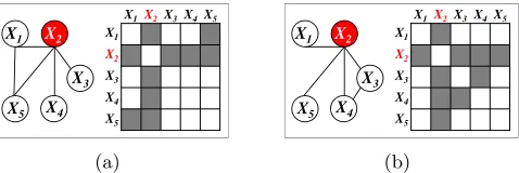
2. The networks differ due to particular nodes that areperturbed across conditions, and

therefore have a completely different connectivity pattern to other nodes in the K

networks. Figure 2 displays a toy example, with p = 5 nodes and K = 2 networks;

here we see that all of the network differences are driven by perturbation in the

second variable, X2. In the context of transcriptional regulatory networks,X2 might

represent a gene that is mutated in a particular condition, effectively disrupting its

conditional dependence relationships with other genes. We propose theperturbed-node

joint graphical lasso (PNJGL), a convex optimization problem for estimating GGMs in this context.

Node-based learning of multiple GGMs is challenging, due to complications resulting from symmetry of the precision matrices. In this paper, we overcome this problem through the use of a new convex regularizer.

X1 X2

X3

X4

X

5

X₅ X₃

X4

X₂

X₁

X1X2X3X4X5

(a)

X1 X2

X3

X4

X

5

X₅ X₃

X4

X₂

X₁

X1X2X3X4X5

(b)

Figure 1: Two networks share a common hub (co-hub) node. X2 serves as a hub node in

both networks. (a): Network 1 and its adjacency matrix. (b): Network 2 and its

adjacency matrix.

The rest of this paper is organized as follows. We introduce some relevant background

material in Section 2. In Section 3, we present the row-column overlap norm (RCON), a

regularizer that encourages a matrix to have a support that is the union of a set of rows

X1

X2

X3

X4

X5 X5

X3

X4 X2

X1X2X3 X4X5 X1

(a)

X1

X2

X3

X4

X5 X5

X3

X4 X2 X1

X1X2X3X4X5

(b)

X1

X2

X3

X4

X5 X5

X3

X4 X2 X1

X1X2X3X4X5

(c)

Figure 2: Two networks that differ due to node perturbation of X2. (a): Network 1 and

its adjacency matrix. (b): Network 2 and its adjacency matrix. (c): Left: Edges

that differ between the two networks. Right: Shaded cells indicate edges that

differ between Networks 1 and 2.

and PNJGL formulations just described. In Section 4, we propose analternating direction

method of multipliers (ADMM) algorithm in order to solve these two convex formulations. In order to scale this algorithm to problems with many variables, in Section 5 we introduce a set of simple conditions on the regularization parameters that indicate that the problem can be broken down into many independent subproblems, leading to substantial algorithm speed-ups. In Section 6, we apply CNJGL and PNJGL to synthetic data, and in Section 7 we apply them to gene expression data and to webpage data. The Discussion is in Section 8. Proofs are in the Appendix.

A preliminary version of some of the ideas in this paper appear in Mohan et al. (2012). There the PNJGL formulation was proposed, along with an ADMM algorithm. Here we expand upon that formulation and present the CNJGL formulation, an ADMM algorithm for solving it, as well as comprehensive results on both real and simulated data. Further-more, in this paper we discuss theoretical conditions for computational speed-ups, which are critical to application of both PNJGL and CNJGL to data sets with many variables.

2. Background on High-Dimensional GGM Estimation

In this section, we review the literature on learning Gaussian graphical models.

2.1 The Graphical Lasso for Estimating a Single GGM

As was mentioned in Section 1, estimating a single GGM on the basis of n independent

and identically distributed observations from a Np(0,Σ) distribution amounts to learning the sparsity structure of Σ−1 (Mardia et al., 1979; Lauritzen, 1996). Whenn > p, one can

estimate Σ−1 by maximum likelihood. But in high dimensions when p is large relative to

n, this is not possible because the empirical covariance matrix is singular. Consequently, a number of authors (among others, Yuan and Lin, 2007a; Friedman et al., 2007; Ravikumar et al., 2008; Banerjee et al., 2008; Scheinberg et al., 2010; Hsieh et al., 2011) have considered maximizing the penalized log likelihood

maximize

Θ∈_Sp₊₊ {log det Θ−trace(SΘ)−λkΘk1}, (1)

where S is the empirical covariance matrix, λ is a nonnegative tuning parameter, Sp++

to (1) serves as an estimate of Σ−1, and a zero element in the solution corresponds to a pair of variables that are estimated to be conditionally independent. Due to the`1 penalty (Tibshirani, 1996) in (1), this estimate will be positive definite for any λ > 0, and sparse when λ is sufficiently large. We refer to (1) as the graphical lasso. Problem (1) is convex, and efficient algorithms for solving it are available (among others, Friedman et al., 2007; Banerjee et al., 2008; Rothman et al., 2008; D’Aspremont et al., 2008; Scheinberg et al., 2010; Witten et al., 2011).

2.2 The Joint Graphical Lasso for Estimating Multiple GGMs

Several formulations have recently been proposed for extending the graphical lasso (1) to the setting in which one has access to a number of observations fromK distinct conditions, each with measurements on the same set ofpvariables. The goal is to estimate a graphical model

for each condition under the assumption that theK networks share certain characteristics

but are allowed to differ in certain structured ways. Guo et al. (2011) take a non-convex approach to solving this problem. Zhang and Wang (2010) take a convex approach, but use a least squares loss function rather than the negative Gaussian log likelihood. Here we review the convex formulation of Danaher et al. (2013), which forms the starting point for the proposal in this paper.

Suppose that X₁k, . . . , X_nk_k ∈ _Rp _{are independent and identically distributed from a}

Np(0,Σk) distribution, for k= 1, . . . , K. Here nk is the number of observations in the kth condition, or class. LettingSk denote the empirical covariance matrix for thekth class, we can maximize the penalized log likelihood

maximize

Θ1_∈

Sp++,...,ΘK∈S

p

++ 





L(Θ1, . . . ,ΘK)−λ1

K X

k=1

kΘkk1−λ2

X

i6=j

P(Θ1_ij, . . . ,ΘK_ij) 





, (2)

where L(Θ1, . . . ,ΘK) = PK

k=1nk log det Θk−trace(SkΘk)

, λ1 and λ2 are nonnegative

tuning parameters, and P(Θ1_ij, . . . ,ΘK_ij) is a convex penalty function applied to each off-diagonal element of Θ1, . . . ,ΘK in order to encourage similarity among them. Then the

ˆ

Θ1, . . . ,ΘˆK that solve (2) serve as estimates for (Σ1)−1, . . . ,(ΣK)−1. Danaher et al. (2013) refer to (2) as thejoint graphical lasso(JGL). In particular, they consider the use of afused lasso penalty (Tibshirani et al., 2005),

P(Θ1_ij, . . . ,ΘK_ij) = X k<k0

|Θk_ij−Θk_ij0|, (3)

on the differences between pairs of network edges, as well as a group lasso penalty (Yuan

and Lin, 2007b),

P(Θ1_ij,Θ2_ij, . . . ,ΘK_ij) = v u u t

K X

k=1

(Θk_ij)2_{, (4)}

on the edges themselves. Danaher et al. (2013) refer to problem (2) combined with (3) as thefused graphical lasso (FGL), and to (2) combined with (4) as thegroup graphical lasso

FGL encourages the K network estimates to have identical edge values, whereas GGL

encourages the K network estimates to have a shared pattern of sparsity. Both the FGL

and GGL optimization problems are convex. An approach related to FGL and GGL is proposed in Hara and Washio (2013).

Because FGL and GGL borrow strength across all available observations in estimating each network, they can lead to much more accurate inference than simply learning each of

theK networks separately.

But both FGL and GGL take an edge-based approach: they assume that differences

between and similarities among the networks arise from individual edges. In this paper,

we propose a node-based formulation that allows for more powerful estimation of multiple

GGMs, under the assumption that network similarities and differences arise from nodes

whose connectivity patterns to other nodes are shared or disrupted across conditions.

3. Node-Based Joint Graphical Lasso

In this section, we first discuss the failure of a naive approach for node-based learning of multiple GGMs. We then present a norm that will play a critical role in our formulations for this task. Finally, we discuss two approaches for node-based learning of multiple GGMs.

3.1 Why is Node-Based Learning Challenging?

At first glance, node-based learning of multiple GGMs seems straightforward. For instance,

consider the task of estimatingK = 2 networks under the assumption that the connectivity

patterns of individual nodes differ across the networks. It seems that we could simply modify (2) combined with (3) as follows,

maximize

Θ1_∈

Sp++,Θ2∈S

p

++ 





L(Θ1,Θ2)−λ1kΘ1k1−λ1kΘ2k1−λ2

p X

j=1

kΘ1_j −Θ2_jk₂







, (5)

where Θk_j is thejth column of the matrix Θk. This amounts to applying agroup lasso(Yuan

and Lin, 2007b) penalty to the columns of Θ1−Θ2. Equation (5) seems to accomplish our

goal of encouraging Θ1_j = Θ2_j. We will refer to this as the naive group lasso approach. In (5), we have applied the group lasso usingp groups; thejth group is thejth column of Θ1−Θ2. Due to the symmetry of Θ1 and Θ2, there is substantial overlap among the p

groups: the (i, j)th element of Θ1−Θ2 is contained in both theith andjth groups. In the presence of overlapping groups, the group lasso penalty yields estimates whosesupport is the complement of the union of groups (Jacob et al., 2009; Obozinski et al., 2011). Figure 3(a) displays a simple example of the results obtained if we attempt to estimate (Σ1)−1−(Σ2)−1 using (5). The figure reveals that (5) cannot be used to detect node perturbation.

A naive approach to co-hub detection is challenging for a similar reason. Recall that the

jth node is a co-hub if thejth columns of both Θ1 and Θ2 contain predominantly non-zero elements, and let diag(Θ) denote a matrix consisting of the diagonal elements of Θ. It is tempting to formulate the optimization problem

maximize

Θ1_∈

Sp++,Θ2∈S

p

++ 





L(Θ1,Θ2)−λ1kΘ1k₁−λ1kΘ2k₁−λ2

p X

j=1

Θ1−diag(Θ1) Θ2−diag(Θ2)

j

2







X1 X2 X3 X4 X5

X1

X2

X3

X4

X5

(a) Naive group lasso

X1 X2 X3 X4 X5

X1

X2

X3

X4

X5

(b) RCON:`1/`1

X1 X2 X3 X4 X5

X1

X2

X3

X4

X5

(c) RCON:`1/`2

X1 X2 X3 X4 X5

X1

X2

X3

X4

X5

(d) RCON:`1/`∞

Figure 3: Toy example of the results from applying various penalties in order to estimate a

5×5 matrix, under a symmetry constraint. Zero elements are shown in white;

non-zero elements are shown in shades of red (positive elements) and blue (negative

elements). (a): The naive group lasso applied to the columns of the matrix

yields non-zero elements that are theintersection, rather than theunion, of a set

of rows and columns. (b): The RCON penalty using an `1/`1 norm results in

unstructured sparsity in the estimated matrix. (c): The RCON penalty using

an `1/`2 norm results in entire rows and columns of non-zero elements. (d):

The RCON penalty using an `1/`∞ norm results in entire rows and columns of

non-zero elements; many take on a single maximal (absolute) value.

where the group lasso penalty encourages the off-diagonal elements of many of the columns to be simultaneously zero in Θ1 and Θ2. Unfortunately, once again, the presence of over-lapping groups encourages the support of the matrices Θ1 and Θ2 to be the intersection of a set of rows and columns, as in Figure 3(a), rather than the union of a set of rows and columns.

3.2 Row-Column Overlap Norm

Detection of perturbed nodes or co-hub nodes requires a penalty function that, when applied to a matrix, yields a support given by the union of a set of rows and columns. We now

propose the row-column overlap norm (RCON) for this task.

Definition 1 The row-column overlap norm (RCON) induced by a matrix norm k.k is de-fined as

Ω(Θ1,Θ2, . . . ,ΘK) = min V1_,V2_,...,VK



   

V1 V2 .. . VK



   

It is easy to check that Ω is indeed a norm for all matrix norms k.k. Also, whenk.k is symmetric in its argument, that is, kVk=kVTk, then

Ω(Θ1,Θ2, . . . ,ΘK) = 1 2 

   

Θ1 Θ2 .. .

ΘK



   

.

Thus if k · kis an `1/`1 norm, then Ω(Θ1,Θ2, . . . ,ΘK) = 1₂PK k=1

P

i,j|Θkij|.

We now discuss the motivation behind Definition 1. Any symmetric matrix Θk can be

(non-uniquely) decomposed as Vk+ (Vk)T; note that Vk need not be symmetric. This

amounts to interpreting Θk as a set of columns (the columns of Vk) plus a set of rows

(the columns of Vk, transposed). In this paper, we are interested in the particular case of RCON penalties wherek.kis an`1/`qnorm, given bykVk=

Pp

j=1kVjkq, where 1≤q ≤ ∞. With a little abuse of notation, we will let Ωqdenote Ω whenk.kis given by the`1/`qnorm. Then Ωqencourages Θ1,Θ2, . . . ,ΘKto decompose intoVkand (Vk)T such that the summed

`q norms of all of the columns (concatenated over V1, . . . , VK) is small. This encourages structures of interest on the columns and rows of Θ1,Θ2, . . . ,ΘK.

To illustrate this point, in Figure 3 we display schematic results obtained from estimating a 5×5 matrix subject to the RCON penalty Ωq, forq= 1, 2, and∞. We see from Figure 3(b)

that when q = 1, the RCON penalty yields a matrix estimate with unstructured sparsity;

recall that Ω1amounts to an`1penalty applied to the matrix entries. Whenq= 2 orq =∞,

we see from Figures 3(c)-(d) that the RCON penalty yields a sparse matrix estimate for

which the non-zero elements are a set of rows plus a set of columns—that is, the union of

a set of rows and columns.

We note that Ω2 can be derived from the overlap norm (Obozinski et al., 2011; Jacob

et al., 2009) applied to groups given by rows and columns of Θ1_{, . . . ,Θ}K_{. Details are} described in Appendix E. Additional properties of RCON are discussed in Appendix A.

3.3 Node-Based Approaches for Learning GGMs

We discuss two approaches for node-based learning of GGMs. The first promotes networks whose differences are attributable to perturbed nodes. The second encourages the networks to share co-hub nodes.

3.3.1 Perturbed-node Joint Graphical Lasso

Consider the task of jointly estimating K precision matrices by solving

maximize

Θ1_,Θ2_,...,ΘK_∈

Sp++ (

L(Θ1,Θ2, . . . ,ΘK)−λ1

K X

k=1

kΘkk1−λ2

X

k<k0

Ωq(Θk−Θk0) )

. (6)

We refer to the convex optimization problem (6) as the perturbed-node joint graphical

lasso (PNJGL). Let ˆΘ1,Θˆ2, . . . ,ΘˆK denote the solution to (6); these serve as estimates for (Σ1)−1, . . . ,(ΣK)−1. In (6), λ1 and λ2 are nonnegative tuning parameters, and q ≥1.

to each condition separately in order to separately estimate K networks. When λ2 > 0,

we are encouraging similarity among the K network estimates. When q = 1, we have the

following observation.

Remark 2 The FGL formulation (Equations 2 and 3) is a special case of PNJGL (6) with q= 1.

In other words, when q = 1, (6) amounts to the edge-based approach of Danaher et al.

(2013) that encourages many entries of ˆΘk_−Θˆk0 _{to equal zero.}

However, whenq= 2 orq=∞, then (6) amounts to anode-based approach: the support

of ˆΘk−Θˆk0 is encouraged to be a union of a few rows and the corresponding columns. These can be interpreted as a set of nodes that are perturbed across the conditions. An example

of the sparsity structure detected by PNJGL with q= 2 or q =∞ is shown in Figure 2.

3.3.2 Co-hub Node Joint Graphical Lasso

We now consider jointly estimatingKprecision matrices by solving the convex optimization

problem

maximize Θ1_,Θ2_,...,ΘK∈_Sp

++

(

L(Θ1,Θ2, . . . ,ΘK)−λ1

K

X

k=1

kΘkk1−λ2Ωq(Θ1−diag(Θ1), . . . ,ΘK−diag(ΘK))

)

. (7)

We refer to (7) as the co-hub node joint graphical lasso (CNJGL) formulation. In (7), λ1

and λ2 are nonnegative tuning parameters, and q ≥ 1. When λ2 = 0 then this amounts

to a graphical lasso optimization problem applied to each network separately; however,

when λ2 >0, a shared structure is encouraged among the K networks. In particular, (7)

encourages network estimates that have a common set of hub nodes—that is, it encourages the supports of Θ1,Θ2, . . . ,ΘK to be the same, and the union of a set of rows and columns. CNJGL can be interpreted as a node-based extension of the GGL proposal (given in Equations 2 and 4, and originally proposed by Danaher et al., 2013). While GGL encourages

theK networks to share a common edge support, CNJGL instead encourages the networks

to share a common node support.

We now remark on an additional connection between CNJGL and the graphical lasso.

Remark 3 If q = 1, then CNJGL amounts to a modified graphical lasso on each network separately, with a penalty ofλ1 applied to the diagonal elements, and a penalty ofλ1+λ2/2

applied to the off-diagonal elements.

4. Algorithms

The PNJGL and CNJGL optimization problems (6, 7) are convex, and so can be directly

solved in the modeling environmentcvx(Grant and Boyd, 2010), which calls conic

interior-point solvers such as SeDuMior SDPT3. However, when applied to solve semi-definite

pro-grams, second-order methods such as the interior-point algorithm do not scale well with the problem size.

a group lasso penalty (as in Yuan and Lin, 2007b) in the presence of overlapping groups (Argyriou et al., 2011; Chen et al., 2011; Mosci et al., 2010). Unfortunately, those algorithms cannot be applied to the PNJGL and CNJGL formulations, which involve the RCON penalty rather than simply a standard group lasso with overlapping groups. The RCON penalty is a variant of the overlap norm proposed in Obozinski et al. (2011), and indeed those authors propose an algorithm for minimizing a least squares objective subject to the overlap norm. However, in the context of CNJGL and PNJGL, the objective of interest is a Gaussian log likelihood, and the algorithm of Obozinski et al. (2011) cannot be easily applied.

Another possible approach for solving (6) and (7) involves the use of a standard first-order method, such as a projected subgradient approach. Unfortunately, such an approach is not straightforward, since computing the subgradients of the RCON penalty involves solving a non-trivial optimization problem (to be discussed in detail in Appendix A). Similarly, a proximal gradient approach for solving (6) and (7) is challenging because the proximal

operator of the combination of the overlap norm and the`1 norm has no closed form.

To overcome the challenges outlined above, we propose to solve the PNJGL and CNJGL

problems using analternating direction method of multipliers algorithm (ADMM; see, e.g.,

Boyd et al., 2010).

4.1 The ADMM Approach

Here we briefly outline the standard ADMM approach for a general optimization problem,

minimize

X g(X) +h(X)

subject to X∈ X. (8)

ADMM is attractive in cases where the proximal operator ofg(X) +h(X) cannot be easily

computed, but where the proximal operator of g(X) and the proximal operator of h(X)

are easily obtained. The approach is as follows (Boyd et al., 2010; Eckstein and Bertsekas, 1992; Gabay and Mercier, 1976):

1. Rewrite the optimization problem (8) as

minimize

X,Y g(X) +h(Y)

subject to X∈ X, X =Y, (9)

where here we have decoupled g and h by introducing a new optimization variable,

Y.

2. Form the augmented Lagrangian to (9) by first forming the Lagrangian,

L(X, Y,Λ) =g(X) +h(Y) +hΛ, X−Yi,

and then augmenting it by a quadratic function ofX−Y,

Lρ(X, Y,Λ) =L(X, Y,Λ) +

ρ

2kX−Yk

2

F,

3. Iterate until convergence:

(a) Update each primal variable in turn by minimizing the augmented Lagrangian with respect to that variable, while keeping all other variables fixed. The updates in thekth iteration are as follows:

Xk+1 ← arg min

X∈XLρ(X, Y k_,Λk_),

Yk+1 ← arg min

Y Lρ(X

k+1_{, Y,Λ}k_).

(b) Update the dual variable using a dual-ascent update,

Λk+1 ← Λk+ρ(Xk+1−Yk+1).

The standard ADMM presented here involves minimization over two primal variables,

X andY. For our problems, we will use a similar algorithm but withmore than two primal

variables. More details about the algorithm and its convergence are discussed in Section 4.2.4.

4.2 ADMM Algorithms for PNJGL and CNJGL

Here we outline the ADMM algorithms for the PNJGL and CNJGL optimization problems; we refer the reader to Appendix F for detailed derivations of the update rules.

4.2.1 ADMM Algorithm for PNJGL

Here we consider solving PNJGL with K = 2; the extension for K > 2 is slightly more

complicated. To begin, we note that (6) can be rewritten as

maximize

Θ1_,Θ2_∈

Sp++,V∈Rp×p 





L(Θ1,Θ2)−λ1kΘ1k1−λ1kΘ2k1−λ2

p X

j=1

kVjkq 





subject to Θ1−Θ2 =V +VT.

(10)

We now reformulate (10) by introducing new variables, so as to decouple some of the terms in the objective function that are difficult to optimize jointly:

minimize

Θ1_∈Sp

++,Θ2∈S

p

++,Z1,Z2,V,W 





−L(Θ1,Θ2) +λ1kZ1k1+λ1kZ2k1+λ2

p X

j=1

kVjkq 





subject to Θ1−Θ2 =V +W, V =WT,Θ1 =Z1,Θ2 =Z2.

(11)

The augmented Lagrangian to (11) is given by

− L(Θ1,Θ2) +λ1kZ1k1+λ1kZ2k1+λ2

p X

j=1

kVjkq+hF,Θ1−Θ2−(V +W)i + hG, V −WTi+hQ1,Θ1−Z1i+hQ2,Θ2−Z2i+ρ₂kΘ1−Θ2−(V +W)k2

F + ρ₂kV −WTk2

F + ρ

2kΘ

1_−Z1_k2

F + ρ

2kΘ

2_−Z2_k2

F.

In (12) there are six primal variables and four dual variables. Based on this augmented Lagrangian, the complete ADMM algorithm for (6) is given in Algorithm 1, in which the operator Expand is given by

Expand(A, ρ, nk) = argmin

Θ∈Sp++

−nklog det(Θ) +ρkΘ−Ak2F =

1 2U

D+ r

D2₊2nk ρ I

UT,

whereU DUT is the eigenvalue decomposition of a symmetric matrix A, and as mentioned

earlier, nk is the number of observations in thekth class. The operatorTq is given by

Tq(A, λ) = argmin X





 1

2kX−Ak

2

F +λ p X

j=1

kXjkq 





,

and is also known as the proximal operator corresponding to the`1/`qnorm. Forq = 1,2,∞, T_q takes a simple form (see, e.g., Section 5 of Duchi and Singer, 2009).

Algorithm 1:ADMM algorithm for the PNJGL optimization problem (6)

input: ρ >0, µ >1, tmax>0;

Initialize: Primal variables to the identity matrix and dual variables to the zero matrix;

for t = 1:tmax do ρ←µρ;

whileNot converged do

Θ1 ←Expand

1

2(Θ2+V +W +Z1)− 1

2ρ(Q1+n1S1+F), ρ, n1

;

Θ2 ←Expand

1

2(Θ1−(V +W) +Z2)− 1

2ρ(Q2+n2S2−F), ρ, n2

;

Zi _{← T}

1

Θi₊Qi ρ,

λ1 ρ

fori= 1,2;

V ← Tq

1

2(WT −W + (Θ1−Θ2)) + 1

2ρ(F−G), λ2

2ρ

;

W ← 1₂(VT −V + (Θ1−Θ2)) + ₂1_ρ(F+GT);

F ←F+ρ(Θ1_−Θ2_{−(V +W));} G←G+ρ(V −WT);

Qi←Qi+ρ(Θi−Zi) for i= 1,2

4.2.2 ADMM Algorithm for CNJGL

The CNJGL formulation in (7) is equivalent to

minimize

Θi_∈

Sp++,Vi∈Rp×p,i=1...K

−L(Θ1,Θ2, . . . ,ΘK) +λ1

K X

i=1

kΘik1+λ2

p X j=1      V1 V2 .. . VK      j q

subject to Θi−diag(Θi) =Vi+ (Vi)T fori= 1, . . . , K.

One can easily see that the problem (13) is equivalent to the problem

minimize

Θi_∈Sp

++,V˜i∈Rp×p,i=1...K

−L(Θ1_,Θ2_{, . . . ,Θ}K_{) +λ}

1

K X

i=1

kΘik1+λ2

p X j=1      ˜

V1_{−diag( ˜V}1₎

˜

V2_{−diag( ˜V}2₎

.. . ˜

VK_{−diag( ˜V}K₎      j _q

subject to Θi_{= ˜V}i_{+ ( ˜V}i₎T _{fori= 1,2, . . . , K,}

(14)

in the sense that the optimal solution {Vi_{} to (13) and the optimal solution {V}˜i_{} to (14)} have the following relationship: Vi = ˜Vi−diag( ˜Vi) fori= 1,2, . . . , K. We now present an ADMM algorithm for solving (14). We reformulate (14) by introducing additional variables in order to decouple some terms of the objective that are difficult to optimize jointly:

minimize

Θi_∈Sp

++,Zi,V˜i,Wi∈Rp×p

−L(Θ1,Θ2, . . . ,ΘK) +λ1

K X

i=1

kZik1+λ2

p X j=1      ˜

V1_{−diag( ˜V}1₎

˜

V2_{−diag( ˜V}2₎

.. . ˜

VK_{−diag( ˜V}K₎      j q

subject to Θi= ˜Vi+Wi,V˜i= (Wi)T,Θi=Zifori= 1,2, . . . , K.

(15)

The augmented Lagrangian to (15) is given by

K X

i=1

ni(−log det(Θi) + trace(SiΘi)) +λ1

K X

i=1

kZik1+λ2

p X j=1      ˜

V1_{−diag( ˜V}1₎

˜

V2_{−diag( ˜V}2₎

.. . ˜

VK_{−diag( ˜V}K₎      j _q + K X i=1 n

hFi,Θi−( ˜Vi+Wi)i+hGi,V˜i−(Wi)Ti+hQi,Θi−Ziio +

ρ 2 K X i=1 n

kΘi−( ˜Vi+Wi)k2

F+kV˜

i_−(Wi₎T_k2

F +kΘ

i_−Zi_k2

F o

.

The corresponding ADMM algorithm is given in Algorithm 2.

Algorithm 2:ADMM algorithm for the CNJGL optimization problem (7)

input: ρ >0, µ >1, tmax>0;

Initialize: Primal variables to the identity matrix and dual variables to the zero matrix;

for t = 1:tmax do ρ←µρ;

whileNot converged do

Θi ←Expand1₂( ˜Vi+Wi+Zi)− 1 2ρ(Q

i_+n

iSi+Fi), ρ, ni

fori=

1, . . . , K;

Zi ← T1

Θi+Q_ρi,λ1 ρ

fori= 1, . . . , K;

LetCi= 1₂((Wi)T −Wi+ Θi) +₂1_ρ(Fi−Gi) for i= 1, . . . , K;      ˜ V1 ˜ V2 .. . ˜ VK     

← Tq

         

C1−diag(C1)

C2_−diag(C2₎

.. .

CK_−diag(CK₎ 

   

,λ2

2ρ      +     

diag(C1) diag(C2₎

.. . diag(CK₎

     ;

Wi _← 1

2(( ˜Vi)T −V˜i+ Θi) + 1

2ρ(Fi+ (Gi)T) for i= 1, . . . , K;

Fi ←Fi+ρ(Θi−( ˜Vi+Wi)) fori= 1, . . . , K;

Gi←Gi+ρ( ˜Vi−(Wi)T) fori= 1, . . . , K;

Qi←Qi+ρ(Θi−Zi) for i= 1, . . . , K

4.2.3 Numerical Issues and Run-Time of the ADMM Algorithms

We set µ = 5, ρ = 0.5 and tmax = 1000 in the PNJGL and CNJGL algorithms. In our

implementation of these algorithms, the stopping criterion for the inner loop (corresponding to a fixedρ) is

max i∈{1,2,...,K}

(

k(Θi)(k+1)−(Θi)(k)k_F k(Θi₎(k)_k

F

)

≤,

where (Θi)(k) denotes the estimate of Θi in thekth iteration of the ADMM algorithm, and

is a tolerance that is chosen in our experiments to equal 10−4.

The per-iteration complexity of the ADMM algorithms for CNJGL and PNJGL (with

K = 2) is O(p3); this is the complexity of computing the SVD. On the other hand, the

complexity of a general interior point method is O(p6). In a small example with p = 30,

run on an Intel Xeon X3430 2.4Ghz CPU, the interior point method (usingcvx, which calls

Sedumi) takes 7 minutes to run, while the ADMM algorithm for PNJGL, coded inMatlab, takes only 0.58 seconds. Whenp= 50, the times are 3.5 hours and 2.1 seconds, respectively. Let ˆΘ1,Θˆ2 and ¯Θ1,Θ¯2 denote the solutions obtained by ADMM andcvx, respectively. We observe that on average, the error max

i∈{1,2} n

kΘˆi−Θ¯ikF/kΘ¯ikF o

We now present a more extensive runtime study for the ADMM algorithms for PNJGL

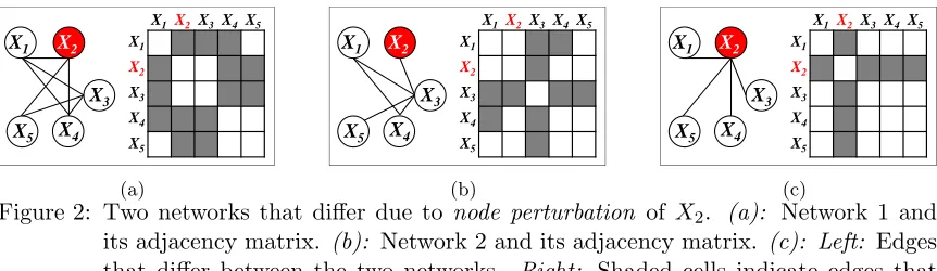
and CNJGL. We ran experiments with p = 100,200,500 and with n1 = n2 = p/2. We

generated synthetic data as described in Section 6. Results are displayed in Figures 4(a)-(d), where the panels depict the run-time and number of iterations required for the algorithm to terminate, as a function ofλ1, and withλ2 fixed. The number of iterations required for the algorithm to terminate is computed as the total number of inner loop iterations performed

in Algorithms 1 and 2. From Figures 4(b) and (d), we observe that aspincreases from 100

to 500, the run-times increase substantially, but never exceed several minutes.

Figure 4(a) indicates that for CNJGL, the total number of iterations required for

algo-rithm termination is small when λ1 is small. In contrast, for PNJGL, Figure 4(c) indicates

that the total number of iterations is large whenλ1 is small. This phenomenon results from

the use of the identity matrix to initialize the network estimates in the ADMM algorithms: when λ1 is small, the identity is a poor initialization for PNJGL, but a good initialization

for CNJGL (since for CNJGL,λ2 induces sparsity even when λ1 = 0).

10−5 10−4 10−3 10−2 10−1 100 50

100 150 200 250 300 350

λ

1

Total num. iterations

p = 100 p = 200 p = 500

(a) CNJGL

100−5 10−4 10−3 10−2 10−1 100 50

100 150 200 250

λ

1

Run time

p = 100 p = 200 p = 500

(b) CNJGL

10−5 10−4 10−3 10−2 10−1 100

0 200 400 600 800

λ

1

Total num. iterations

p = 100 p = 200 p = 500

(c) PNJGL

100−5 10−4 10−3 10−2 10−1 100 100

200 300 400 500

λ

1

Run time

p = 100 p = 200 p = 500

(d) PNJGL

Figure 4: (a): The total number of iterations for the CNJGL algorithm, as a function of

λ1. (b): Run-time (in seconds) of the CNJGL algorithm, as a function of λ1.

4.2.4 Convergence of the ADMM Algorithm

Problem (9) involves two (groups of) primal variables,XandY; in this setting, convergence of ADMM has been established (see, e.g., Boyd et al., 2010; Mota et al., 2011). However, the PNJGL and CNJGL optimization problems involve more than two groups of primal variables, and convergence of ADMM in this setting is an ongoing area of research. Indeed, as mentioned in Eckstein (2012), the standard analysis for ADMM with two groups does not extend in a straightforward way to ADMM with more than two groups of variables. Han and Yuan (2012) and Hong and Luo (2012) show convergence of ADMM with more than two groups of variables under assumptions that do not hold for CNJGL and PNJGL. Under very minimal assumptions, He et al. (2012) proved that a modified ADMM algorithm (with Gauss-Seidel updates) converges to the optimal solution for problems with any number of groups. More general conditions for convergence of the ADMM algorithm with more than two groups is left as a topic for future work. We also leave for future work a reformulation of the CNJGL and PNJGL problems as consensus problems, for which an ADMM algorithm involving two groups of primal variables can be obtained, and for which convergence would be guaranteed. Finally, note that despite the lack of convergence theory, ADMM with more than two groups has been used in practice and often observed to converge faster than other variants. As an example see Tao and Yuan (2011), where their ASALM algorithm (which is the same as ADMM with more than two groups) is reported to be significantly faster than a variant with theoretical convergence.

5. Algorithm-Independent Computational Speed-Ups

The ADMM algorithms presented in the previous section work well on problems of moder-ate size. In order to solve the PNJGL or CNJGL optimization problems when the number of variables is large, a faster approach is needed. We now describe conditions under which any algorithm for solving the PNJGL or CNJGL problems can be sped up substantially, for an appropriate range of tuning parameter values. Our approach mirrors previous results for the graphical lasso (Witten et al., 2011; Mazumder and Hastie, 2012), and FGL and GGL (Danaher et al., 2013). The idea is simple: if the solutions to the PNJGL or CNJGL opti-mization problem are block-diagonal (up to some permutation of the variables) with shared support, then we can obtain the global solution to the PNJGL or CNJGL optimization problem by solving the PNJGL or CNJGL problem separately on the variables within each block. This can lead to massive speed-ups. For instance, if the solutions are block-diagonal

with L blocks of equal size, then the complexity of our ADMM algorithm reduces from

O(p3) per iteration, to O((p/L)3) per iteration in each of L independent subproblems. Of course, this hinges upon knowing that the PNJGL or CNJGL solutions are block-diagonal, and knowing the partition of the variables into blocks.

In Sections 5.1-5.3 we derive necessary and sufficient conditions for the solutions to the PNJGL and CNJGL problems to be block-diagonal. Our conditions depend only on the sample covariance matrices S1, . . . , Sk and regularization parameters λ1, λ2. These

conditions can be applied in at most O(p2) operations. In Section 5.4, we demonstrate the speed-ups that can result from applying these sufficient conditions.

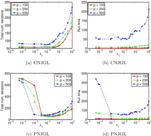
Figure 5: Ap×pmatrix is displayed, for whichI1, I2, I3 denote a partition of the index set

{1,2, . . . , p}. T =SL

i=1{Ii×Ii} is shown in red, and Tcis shown in gray.

and sufficient for the solution to be block diagonal. In contrast, in the results derived below, there is a gap between the necessary and sufficient conditions. Though only the sufficient conditions are required in order to obtain the computational speed-ups discussed in Section 5.4, knowing the necessary conditions allows us to get a handle on the tightness (and, consequently, the practical utility) of the sufficient conditions, for a particular value of the tuning parameters.

We now introduce some notation that will be used throughout this section. Let

(I1, I2, . . . , IL) be a partition of the index set {1,2, . . . , p}, and let T = SLi=1{Ii ×Ii}. Define thesupport of a matrix Θ, denoted by supp(Θ), as the set of indices of the non-zero

entries in Θ. We say Θ is supported onT if supp(Θ)⊆T . Note that any matrix supported

on T is block-diagonal subject to some permutation of its rows and columns. Let |T|

de-note the cardinality of the set T, and letTc denote the complement ofT. The scheme is

displayed in Figure 5. In what follows we use an `1/`q norm in the RCON penalty, with

q≥1, and let 1_s +1_q = 1.

5.1 Conditions for PNJGL Formulation to Have Block-Diagonal Solutions

In this section, we give necessary conditions and sufficient conditions on the regularization parametersλ1, λ2in the PNJGL problem (6) so that the resulting precision matrix estimates

ˆ

Θ1, . . . ,ΘˆK have a shared block-diagonal structure (up to a permutation of the variables). We first present a necessary condition for ˆΘ1 and ˆΘ2 that minimize (6) with K = 2 to be block-diagonal.

Theorem 4 Suppose that the matrices Θˆ1 and Θˆ2 that minimize (6) with K = 2 have support T. Then, if q≥1, it must hold that

nk|Sijk| ≤λ1+λ2/2 ∀(i, j)∈Tc, fork= 1,2, and (17)

|n1S_ij1 +n2S_ij2| ≤2λ1 ∀(i, j)∈Tc. (18)

Furthermore, ifq >1, then it must additionally hold that

nk |Tc_|

X

(i,j)∈Tc

|S_ijk| ≤λ1+ λ2

2

p

|Tc_| 1/s

, fork= 1,2. (19)

Remark 5 If|Tc|=O(pr)withr >1, then asp→ ∞, (19) simplifies to nk |Tc_|

P

We now present a sufficient condition for ˆΘ1, . . . ,ΘˆK that minimize (6) to be block-diagonal.

Theorem 6 For q ≥1, a sufficient condition for the matrices Θˆ1, . . . ,ΘˆK that minimize (6) to each have support T is that

nk|Sijk| ≤λ1 ∀(i, j)∈Tc, fork= 1, . . . , K.

Furthermore, if q = 1 and K = 2, then the necessary conditions (17) and (18) are also sufficient.

When q = 1 andK = 2, then the necessary and sufficient conditions in Theorems 4 and 6

are identical, as was previously reported in Danaher et al. (2013). In contrast, there is a

gap between the necessary and sufficient conditions in Theorems 4 and 6 when q > 1 and

λ2 >0. When λ2 = 0, the necessary and sufficient conditions in Theorems 4 and 6 reduce

to the results laid out in Witten et al. (2011) for the graphical lasso.

5.2 Conditions for CNJGL Formulation to Have Block-Diagonal Solutions

In this section, we give necessary and sufficient conditions on the regularization parame-ters λ1, λ2 in the CNJGL optimization problem (7) so that the resulting precision matrix

estimates ˆΘ1_{, . . . ,Θ}ˆK _{have a shared block-diagonal structure (up to a permutation of the} variables).

Theorem 7 Suppose that the matricesΘˆ1,Θˆ2, . . . ,ΘˆK that minimize (7) have support T. Then, if q≥1, it must hold that

nk|Sijk| ≤λ1+λ2/2 ∀(i, j)∈Tc, fork= 1, . . . , K. Furthermore, ifq >1, then it must additionally hold that

nk |Tc_|

X

(i,j)∈Tc

|S_ijk| ≤λ1+ λ2

2

p

|Tc_| 1/s

, fork= 1, . . . , K. (20)

Remark 8 If|Tc|=O(pr)withr >1, then asp→ ∞, (20) simplifies to nk |Tc_|

P

(i,j)∈Tc|Sk_ij| ≤λ1.

We now present a sufficient condition for ˆΘ1,Θˆ2, . . . ,ΘˆK that minimize (7) to be block-diagonal.

Theorem 9 A sufficient condition for Θˆ1,Θˆ2, . . . ,ΘˆK that minimize (7) to have support T is that

nk|Sijk| ≤λ1 ∀(i, j)∈Tc, fork= 1, . . . , K.

5.3 General Sufficient Conditions

In this section, we give sufficient conditions for the solution to a general class of optimization problems that include FGL, PNJGL, and CNJGL as special cases to be block-diagonal. Consider the optimization problem

minimize

Θ1_,...,ΘK_∈

Sp++

( _K

X

k=1

nk(−log det(Θk) +hΘk, Ski) + K X

k=1

λ1kΘkk1+λ2h(Θ1, . . . ,ΘK)

)

.

(21)

Once again, let T be the support of a p×p block-diagonal matrix. Let ΘT denote the

restriction of any p×p matrix Θ toT; that is, (ΘT)ij = (

Θij if (i, j)∈T

0 else . Assume that

the functionh satisfies

h(Θ1, . . . ,ΘK)> h(Θ1_U, . . . ,ΘK_U) for any matrices Θ1, . . . ,ΘK whose support strictly containsU.

Theorem 10 A sufficient condition for the matrices Θˆ1_{, . . . ,Θ}ˆK _{that solve (21) to have}

support T is that

nk|Sijk| ≤λ1 ∀(i, j)∈Tc, fork= 1, . . . , K.

Note that this sufficient condition applies to a broad class of regularizers h; indeed, the sufficient conditions for PNJGL and CNJGL given in Theorems 6 and 9 are special cases of Theorem 10. In contrast, the necessary conditions for PNJGL and CNJGL in Theorems 4 and 7 exploit the specific structure of the RCON penalty.

5.4 Evaluation of Speed-Ups on Synthetic Data

Theorems 6 and 9 provide sufficient conditions for the precision matrix estimates from PNJGL or CNJGL to be block-diagonal with a given support. How can these be used in

order to obtain computational speed-ups? We construct ap×pmatrix Awith elements

Aij = 

 

 

1 if i=j

1 if nk|Sijk|> λ1 for anyk= 1, . . . , K

0 else

.

We can then check, in O(p2) operations, whether A is (subject to some permutation of

the rows and columns) block-diagonal, and can also determine the partition of the rows and columns corresponding to the blocks (see, e.g., Tarjan, 1972). Then, by Theorems 6 and 9, we can conclude that the PNJGL or CNJGL estimates are block-diagonal, with the same partition of the variables into blocks. Inspection of the PNJGL and CNJGL optimization problems reveals that we can then solve the problems on the variables within each block separately, in order to obtain the global solution to the original PNJGL or CNJGL optimization problems.

We now investigate the speed-ups that result from applying this approach. We consider

the problem of estimating two networks of size p= 500. We create two inverse covariance

block. We then generate n1 = 250 observations from a multivariate normal distribution

with the first covariance matrix, and n2 = 250 observations from a multivariate normal

distribution with the second covariance matrix. These observations are used to generate

sample covariance matricesS1andS2. We then performed CNJGL and PNJGL withλ2 = 1

and a range of λ1 values, with and without the computational speed-ups just described.

Figure 6 displays the performance of the CNJGL and PNJGL formulations, averaged over 20 data sets generated in this way. In each panel, thex-axis shows the number of blocks into which the optimization problems were decomposed using the sufficient conditions; note

that this is a surrogate for the value ofλ1 in the CNJGL or PNJGL optimization problems.

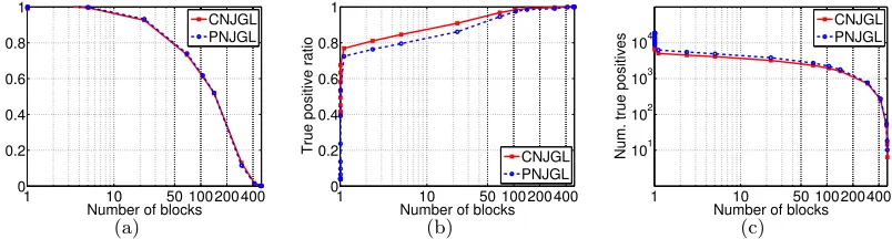
Figure 6(a) displays the ratio of the run-time taken by the ADMM algorithm when exploiting the sufficient conditions to the run-time when not using the sufficient conditions. Figure 6(b) displays the true-positive ratio—that is, the ratio of the number of true positive edges in the precision matrix estimates to the total number of edges in the precision matrix estimates. Figure 6(c) displays the total number of true positives for the CNJGL and PNJGL estimates. Figure 6 indicates that the sufficient conditions detailed in this section lead to substantial computational improvements.

1 10 50 100 200 400 0

0.2 0.4 0.6 0.8 1

Number of blocks

Ratio of run times

CNJGL PNJGL

(a)

1 10 50 100200400

0 0.2 0.4 0.6 0.8 1

Number of blocks

True positive ratio _CNJGL

PNJGL

(b)

1 10 50 100200400

101 102 103 104

Number of blocks

Num. true positives

CNJGL PNJGL

(c)

Figure 6: Speed-ups for CNJGL and PNJGL on a simulation set-up with p = 500 and

n1 = n2 = 250. The true inverse covariance matrices are block-diagonal with

two equally-sized sparse blocks. The x-axis in each panel displays the number

of blocks into which the CNJGL or PNJGL problems are decomposed using the sufficient conditions; this is a surrogate forλ1. The y-axes display(a): the ratio

of run-times with and without the sufficient conditions; (b): the true positive

ratio of the edges estimated; and (c): the total number of true positive edges

estimated.

6. Simulation Study

In this section, we present the results of a simulation study demonstrating the empirical performance of PNJGL and CNJGL.

6.1 Data Generation

In the simulation study, we generated two synthetic networks (either Erdos-Renyi,

were then modified in order to create two perturbed nodes and two co-hub nodes. Details are provided in Sections 6.1.1-6.1.3.

6.1.1 Data Generation for Erdos-Renyi Network

We generated the data as follows, for p= 100, and n∈ {25,50,100,200}:

Step 1: To generate an Erdos-Renyi network, we created ap×p symmetric matrix

A with elements

Aij ∼i.i.d.

0 with probability 0.98,

Unif([−0.6,−0.3]∪[0.3,0.6]) otherwise.

Step 2: We duplicated A into two matrices, A1 and A2. We selected two nodes at random, and for each node, we set the elements of the corresponding row and column of either A1 orA2 (chosen at random) to be i.i.d. draws from a Unif([−0.6,−0.3]∪ [0.3,0.6]) distribution. This results in two perturbed nodes.

Step 3: We randomly selected two nodes to serve as co-hub nodes, and set each element of the corresponding rows and columns in each network to be i.i.d. draws from a Unif([−0.6,−0.3]∪[0.3,0.6]) distribution. In other words, these co-hub nodes areidentical across the two networks.

Step 4: In order to make the matrices positive definite, we let c =

min(λmin(A1), λmin(A2)), whereλmin(·) indicates the smallest eigenvalue of the matrix.

We then set (Σ1₎−1 _{equal toA}1_{+ (0.1 +|c|)I and set (Σ}2₎−1 _{equal toA}2_{+ (0.1 +|c|)I,}

whereI is the p×p identity matrix.

Step 5: We generated n independent observations each from a N(0,Σ1) and a

N(0,Σ2_{) distribution, and used them to compute the sample covariance matrices}

S1 and S2.

6.1.2 Data Generation for Scale-free Network

The data generation proceeded as in Section 6.1.1, except that Step 1 was modified:

Step 1: We used the SFNG functions in Matlab (George, 2007) with parameters

mlinks=2and seed=1to generate a scale-free network withpnodes. We then created ap×psymmetric matrixAthat has non-zero elements only for the edges in the scale-free network. These non-zero elements were generated i.i.d. from a Unif([−0.6,−0.3]∪ [0.3,0.6]) distribution.

Steps 2-5 proceeded as in Section 6.1.1.

6.1.3 Data Generation for Community Network

Then A1 and A2 have non-zero entries concentrated in the top and bottom 60×60 principal submatrices. These two submatrices correspond to two communities. Twenty nodes overlap between the two communities.

6.2 Results

We now define several metrics used to measure algorithm performance. We wish to quantify each algorithm’s (1) recovery of the support of the true inverse covariance matrices, (2)

successful detection of co-hub and perturbed nodes, and (3) error in estimation of Θ1 =

(Σ1)−1 and Θ2 = (Σ2)−1. Details are given in Table 1. These metrics are discussed further

in Appendix G.

We compared the performance of PNJGL to its edge-based counterpart FGL, as well as to graphical lasso (GL). We compared the performance of CNJGL to GGL and GL. We expect CNJGL to be able to detect co-hub nodes (and, to a lesser extent, perturbed nodes), and we expect PNJGL to be able to detect perturbed nodes. (The co-hub nodes will not be detected by PNJGL, since they are identical across the networks.)

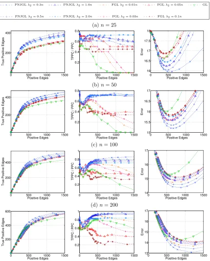
The simulation results for the set-up of Section 6.1.1 are displayed in Figures 7 and 8. Each row corresponds to a sample size while each column corresponds to a performance metric. In Figure 7, PNJGL, FGL, and GL are compared, and in Figure 8, CNJGL, GGL,

and GL are compared. Within each plot, each colored line corresponds to the results

obtained using a fixed value of λ2 (for either PNJGL, FGL, CNJGL, or GGL), as λ1 is

varied. Recall that GL corresponds to any of these four approaches withλ2 = 0. Note that

the number of positive edges (defined in Table 1) decreases approximately monotonically with the regularization parameterλ1, and so on the x-axis we plot the number of positive edges, rather than λ1, for ease of interpretation.

In Figure 7, we observe that PNJGL outperforms FGL and GL for a suitable range of the regularization parameter λ2, in the sense that for a fixed number of edges estimated,

PNJGL identifies more true positives, correctly identifies a greater ratio of perturbed nodes,

and yields a lower Frobenius error in the estimates of Θ1 and Θ2. In particular, PNJGL

performs best relative to FGL and GL when the number of samples is the smallest, that is, in the high-dimensional data setting. Unlike FGL, PNJGL fully exploits the fact that differences between Θ1 and Θ2 are due to node perturbation. Not surprisingly, GL performs worst among the three algorithms, since it does not borrow strength across the conditions in estimating Θ1 and Θ2.

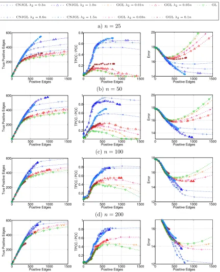
In Figure 8, we note that CNJGL outperforms GGL and GL for a suitable range of the

regularization parameter λ2. In particular, CNJGL outperforms GGL and GL by a larger

margin when the number of samples is the smallest. Once again, GL performs the worst since it does not borrow strength across the two networks; CNJGL performs the best since it fully exploits the presence of hub nodes in the data.

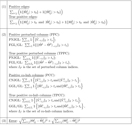
(1) Positive edges:

P i<j

1{|Θˆ1_ij|> t0}+1{|Θˆ2_ij|> t0} True positive edges:

P i<j

1{|Θ1_ij|> t0 and |Θˆ1ij|> t0}+1{|Θ2ij|> t0 and |Θˆ2ij|> t0}

(2) Positive perturbed columns (PPC):

PNJGL: Pp

i=11

n

kVˆ−i,ik2> ts o

;

FGL/GL: Pp

i=11{k( ˆΘ1−Θˆ2)−i,ik2 > ts} True positive perturbed columns (TPPC):

PNJGL: P

i∈Ip1{kVˆ−i,ik2> ts};

FGL/GL: P

i∈Ip1{k( ˆΘ

1_−Θˆ2₎

−i,ik2 > ts}, whereIP is the set of perturbed column indices.

Positive co-hub columns (PCC):

CNJGL: Pp

i=11

n

kVˆ_−i,i1 k₂ > tsandkVˆ−i,i2 k2 > ts o

;

GGL/GL:Pp

i=11

n

kΘˆ1_−i,ik2> tsandkΘˆ2−i,ik2> ts o

True positive co-hub columns (TPCC):

CNJGL: P

i∈Ic1

n

kVˆ_−i,i1 k₂> tsandkVˆ−i,i2 k2 > ts o

;

GGL/GL:P

i∈Ic1

n

kΘˆ1_−i,ik2 > tsandkΘˆ2−i,ik2> ts o

,

whereIC is the set of co-hub column indices.

(3) Error: q

P

i<j(Θ1ij−Θˆ1ij)2+ q

P

i<j(Θ2ij −Θˆ2ij)2

Table 1: Metrics used to quantify algorithm performance. Here Θ1 and Θ2 denote the

true inverse covariance matrices, and ˆΘ1 and ˆΘ2 denote the two estimated inverse

covariance matrices. Here 1{A} is an indicator variable that equals one if the

event A holds, and equals zero otherwise. (1) Metrics based on recovery of the

support of Θ1 and Θ2. Here t0 = 10−6. (2) Metrics based on identification of perturbed nodes and co-hub nodes. The metrics PPC and TPPC quantify node perturbation, and are applied to PNJGL, FGL, and GL. The metrics PCC and TPCC relate to co-hub detection, and are applied to CNJGL, GGL, and GL.

We let ts = µ+ 5.5σ, where µ is the mean and σ is the standard deviation of

{kVˆ−i,ik2}pi=1 (PPC or TPPC for PNJGL),{k( ˆΘ1−Θˆ2)−i,ik2}pi=1 (PPC or TPPC

for FGL/GL), {kVˆ_−i,i1 k₂}p_i=1 and {kVˆ_−i,i2 k₂}p_i=1 (PPC or TPPC for CNJGL), or {kΘˆ1_−i,ik2}p_i=1 and {kΘˆ2−i,ik2}p_i=1 (PPC or TPPC for GGL/GL). However, results

counterparts of CNJGL and PNJGL: when GGL is performed with a large value ofλ2 then

the network estimates are necessarily sparse, regardless of the value ofλ1. But the same is not true for FGL.

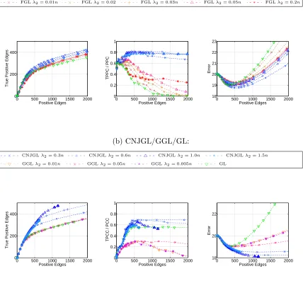
The simulation results for the set-ups of Sections 6.1.2 and 6.1.3 are displayed in Figures

9 and 10, respectively, for the case n= 50. The results show that once again, PNJGL and

CNJGL substantially outperform the edge-based approaches on the three metrics defined earlier.

7. Real Data Analysis

In this section, we present the results of PNJGL and CNJGL applied to two real data sets: gene expression data set and university webpage data set.

7.1 Gene Expression Data

In this experiment, we aim to reconstruct the gene regulatory networks of two subtypes of glioblastoma multiforme (GBM), as well as to identify genes that can improve our under-standing of the disease. Cancer is caused by somatic (cancer-specific) mutations in the genes involved in various cellular processes including cell cycle, cell growth, and DNA repair; such mutations can lead to uncontrolled cell growth. We will show that PNJGL and CNJGL can be used to identify genes that play central roles in the development and progression of cancer. PNJGL tries to identify genes whose interactions with other genes vary significantly between the subtypes. Such genes are likely to have deleterious somatic mutations. CNJGL tries to identify genes that have interactions with many other genes in all subtypes. Such genes are likely to play an important role in controlling other genes’ expression, and are typically calledregulators.

We applied the proposed methods to a publicly available gene expression data set that measures mRNA expression levels of 11,861 genes in 220 tissue samples from patients with

GBM (Verhaak et al., 2010). The raw gene expression data were generated using the

Affymetrix GeneChips technology. We downloaded the raw data in .CEL format from the The Caner Genome Atlas (TCGA) website. The raw data were normalized by using the

Affymetrix MAS5 algorithm, which has been shown to perform well in many studies (Lim

et al., 2007). The data were then log2 transformed and batch-effected corrected using the

softwareComBat(Johnson and Li, 2006). Each patient has one of four subtypes of GBM—

Proneural, Neural, Classical, or Mesenchymal. We selected two subtypes, Proneural (53 tissue samples) and Mesenchymal (56 tissue samples), that have the largest sample sizes. All analyses were restricted to the corresponding set of 109 tissue samples.

To evaluate PNJGL’s ability to identify genes with somatic mutations, we focused on the following 10 genes that have been suggested to be frequently mutated across the four GBM subtypes (Verhaak et al., 2010): TP53, PTEN, NF1, EGFR, IDH1, PIK3R1, RB1, ERBB2, PIK3CA, PDGFRA. We then considered inferring the regulatory network of a set of genes that is known to be involved in a single biological process, based on the Reactome database (Matthews et al., 2008). In particular, we focused our analysis on the “TCR signaling” gene set, which contains the largest number of mutated genes. This gene set contains 34 genes, of which three (PTEN, PIK3R1, and PIK3CA) are in the list of 10 genes suggested to be

- -×- - PNJGLλ2= 0.3n - -4- - PNJGLλ2= 1.0n ·-×-· FGLλ2= 0.01n ·-4-· FGLλ2= 0.05n ·-5-· GL

- -+- - PNJGLλ2= 0.5n - -∗- - PNJGLλ2= 2.0n ·-+-· FGLλ2= 0.03n ·-∗-· FGLλ2= 0.1n

(a)n= 25

0 500 1000 1500

200 400

Positive Edges

True Positive Edges

0 500 1000 1500 0.2

0.4 0.6 0.8

Positive Edges

TPPC / PPC

0 500 1000 1500

16 16.5 17 17.5 18

Positive Edges

Error

(b) n= 50

0 500 1000 1500

200 400

Positive Edges

True Positive Edges

0 500 1000 1500 0.2

0.4 0.6 0.8

Positive Edges

TPPC / PPC

0 500 1000 1500

15 15.5 16 16.5 17

Positive Edges

Error

(c) n= 100

0 500 1000 1500

200 400

Positive Edges

True Positive Edges

0 500 1000 1500 0.2

0.4 0.6 0.8 1

Positive Edges

TPPC / PPC

0 500 1000 1500

14 15 16 17

Positive Edges

Error

(d) n= 200

0 500 1000 1500

200 400 600

Positive Edges

True Positive Edges

0 500 1000 1500 0.2

0.4 0.6 0.8 1

Positive Edges

TPPC / PPC

0 500 1000 1500

13 14 15 16 17

Positive Edges

Error

Figure 7: Simulation results on Erdos-Renyi network (Section 6.1.1) for PNJGL withq= 2,

FGL, and GL, for(a): n = 25, (b): n= 50, (c): n= 100, (d): n= 200, when

p = 100. Each colored line corresponds to a fixed value of λ2, as λ1 is varied.

- -×- - CNJGLλ2= 0.3n - -4- - CNJGLλ2= 1.0n ·-×-· GGLλ2= 0.01n ·-4-· GGLλ2= 0.05n ·-5-· GL

- -+- - CNJGLλ2= 0.6n - -∗- - CNJGLλ2= 1.5n ·-+-· GGLλ2= 0.03n ·-∗-· GGLλ2= 0.1n

a)n= 25

0 500 1000 1500

200 400 600

Positive Edges

True Positive Edges

0 500 1000 1500 0.2

0.4 0.6 0.8

Positive Edges

TPCC / PCC

0 500 1000 1500

14 16 18 20

Positive Edges

Error

(b) n= 50

0 500 1000 1500

200 400 600

Positive Edges

True Positive Edges

0 500 1000 1500 0.2

0.4 0.6 0.8 1

Positive Edges

TPCC / PCC

0 500 1000 1500

14 16 18 20

Positive Edges

Error

(c) n= 100

0 500 1000 1500

200 400 600

Positive Edges

True Positive Edges

0 500 1000 1500 0.2

0.4 0.6 0.8 1

Positive Edges

TPCC / PCC

0 500 1000 1500

12 14 16 18

Positive Edges

Error

(d) n= 200

0 500 1000 1500

200 400 600

Positive Edges

True Positive Edges

0 500 1000 1500 0.2

0.4 0.6 0.8 1

Positive Edges

TPCC / PCC

0 500 1000 1500

12 14 16

Positive Edges

Error

Figure 8: Simulation results on Erdos-Renyi network (Section 6.1.1) for CNJGL withq= 2,

GGL, and GL, for(a): n = 25, (b): n= 50, (c): n= 100, (d): n= 200, when

p = 100. Each colored line corresponds to a fixed value of λ2, as λ1 is varied.

(a) PNJGL/FGL/GL:

- -×- - PNJGLλ2= 0.3n - -+- - PNJGLλ2= 0.5n - -4- - PNJGLλ2= 1.0n - -∗- - PNJGLλ2= 2.0n ·-5-· GL

·-×-· FGLλ2= 0.01n ·-×-· FGLλ2= 0.02 ·-+-· FGLλ2= 0.03n ·-4-· FGLλ2= 0.05n ·-∗-· FGLλ2= 0.2n

0 500 1000 1500 2000

0 200 400

Positive Edges

True Positive Edges

0 500 1000 1500 2000

0 0.2 0.4 0.6 0.8 1

Positive Edges

TPPC / PPC

0 500 1000 1500 2000

18 19 20 21 22 23

Positive Edges

Error

(b) CNJGL/GGL/GL:

- -×- - CNJGLλ2= 0.3n - -+- - CNJGLλ2= 0.6n - -4- - CNJGLλ2= 1.0n - -∗- - CNJGLλ2= 1.5n

·-5-· GGLλ2= 0.01n ·-×-· GGLλ2= 0.05n ·-∗-· GGLλ2= 0.005n ·-5-· GL

0 500 1000 1500 2000

0 200 400

Positive Edges

True Positive Edges

0 500 1000 1500 2000

0 0.2 0.4 0.6 0.8 1

Positive Edges

TPCC / PCC

0 500 1000 1500 2000

18 20 22

Positive Edges

Error

Figure 9: Simulation results on scale-free network (Section 6.1.2) for (a): PNJGL with

q= 2, FGL, and GL, and (b): CNJGL withq = 2, GGL, and GL, with p= 100

andn= 50. Each colored line corresponds to a fixed value ofλ2, asλ1 is varied.

(a) PNJGL/FGL/GL:

- -×- - PNJGLλ2= 0.3n - -+- - PNJGLλ2= 0.5n - -4- - PNJGLλ2= 1.0n - -∗- - PNJGLλ2= 2.0n ·-5-· GL

·-×-· FGLλ2= 0.01n ·-+-· FGLλ2= 0.03 ·-4-· FGLλ2= 0.05n ·-∗-· FGLλ2= 0.2n ·-5-· FGLλ2= 0.5n

0 500 1000 1500 2000

0 200 400

Positive Edges

True Positive Edges

0 500 1000 1500 2000

0 0.2 0.4 0.6 0.8 1

Positive Edges

TPPC / PPC

0 500 1000 1500 2000

19 20 21 22 23

Positive Edges

Error

(b) CNJGL/GGL/GL:

- -×- - CNJGLλ2= 0.3n - -+- - CNJGLλ2= 0.6n - -4- - CNJGLλ2= 1.0n - -∗- - CNJGLλ2= 1.5n

·-×-· GGLλ2= 0.01n ·-+-· GGLλ2= 0.03n ·-4-· GGLλ2= 0.05n ·-5-· GL

0 500 1000 1500 2000

0 200 400

Positive Edges

True Positive Edges

0 500 1000 1500 2000

0 0.2 0.4 0.6 0.8 1

Positive Edges

TPCC / PCC

0 500 1000 1500 2000

19 21 23

Positive Edges

Error

Figure 10: Simulation results on community network (Section 6.1.3) for(a): PNJGL with

q= 2, FGL, and GL, and(b): CNJGL withq= 2, GGL, and GL, withp= 100

andn= 50. Each colored line corresponds to a fixed value ofλ2, asλ1is varied.