http://www.sciencepublishinggroup.com/j/mcs doi: 10.11648/j.mcs.20170202.12
Calculation of the Riemann Zeta-function on a Relativistic
Computer
Yuriy N. Zayko
Department of Applied Informatics, Faculty of Public Administration, The Russian Presidential Academy of National Economy and Public, Administration, Saratov Branch, Saratov, Russia
Email address:
[email protected]To cite this article:
Yuriy N. Zayko. Calculation of the Riemann Zeta-function on a Relativistic Computer. Mathematics and Computer Science. Vol. 2, No. 2, 2017, pp. 20-26. doi: 10.11648/j.mcs.20170202.12
Received: May 10, 2017; Accepted: May 20, 2017; Published: July 6, 2017
Abstract:
The problem of calculating the sum of a divergent series for the Riemann ζ-function of a complex argument is considered in the paper, using the effects of the general theory of relativity. The parameters of the reference frame metric in which the calculation is performed are determined and solutions of the relativistic equations of motion of the material point realizing the calculation are found. The work lies at the junction of the direction known as "Beyond Turing", considering the application of the so-called "relativistic supercomputers" for solving non-computable problems and a direction devoted to the study of non-trivial zeros of the Riemann ζ-function. The formulation of the Riemann hypothesis concerning the distribution of nontrivial zeros of the ζ-function from the point of view of their computability on a relativistic computer is given. In view of the importance of the latter issue for studying the distribution of prime numbers, the results of the work may be of interest to specialists in the field of information security.Keywords:
Metric, Riemann zeta-function, General Theory of Relativity, Space-Time Curvature, Non-computable Problems, Singularity, Black Hole, Relativistic Computer1. Introduction
In this paper, an attempt is made to calculate the Riemann ζ-function using relativistic effects, or, more precisely, effects of the general theory of relativity (GRT). This idea was first used in the author's paper [1], where it was shown that by introducing the corresponding curved metric at the axis of real numbers, one can calculate the sum of a divergent series representing ζ (-1). The relative error obtained in [1] is ~ 3,5%. Note that the talking is about the calculation, and not about some or other methods of summing divergent series [2]. In the present paper, these ideas were used to calculate the ζ-function of a complex argument. To do this, we use the representation of the ζ-function in the form of a series
1
( ) s,
n
s n s u iv
ζ ∞ −
=
=
∑
= +which diverges for u<1 [2]. Calculations were performed foru=1/ 2.
Such an approach (known as "Beyond Turing") to solving
problems beyond the range of problems solved by the classical Turing machine develops in a number of works since the 1980s of the last century (see, for example, [3]). The corresponding computing devices received a name of "relativistic supercomputers". An unchanging attribute of the proposed projects is black holes, as the sources of the metric required for their implementation. The approach developed below, as in the author's previous paper [1], is free from this necessity. The calculation of the sum of a divergent series (a non-computable problem) is regarded as a physical problem about the motion of a material point in curved space-time, which is, in fact, the embodiment of the thesis, which is inverse to the well-known thesis, that any motion of a physical system can be treated as calculation [4]. In the book [4] the role of such a physical system plays the Universe.
2. Behavior of the ζ-function in the
Complex Plane
Consider the behavior on the complex plane of partial sums of the divergent series, representing the Riemann ζ -function (hereinafter, the ζ-function) of the complex argument
1
( )
m s m
n
s n
ζ −
=
=
∑
(1)where n, m are natural numbers, s is an argument. Figure 1 shows the results of calculating ζm。
Figure 1. Calculation results of ζm(s1); s1=0.5-14.134725i - first non-trivial zero of ζ-function [9]. The choice of zero with negative imaginary part is dictated
by considerations of convenience; (a): U = Re [ζm(s1)], V = Im [ζm(s1)]; (b): R=| ζm(s1)|, F= arg[ζm(s1)]; 1< m < 1001.
From Figure 1a it is seen that successive values of ζm for sufficiently large m lie on a curve describing the velocity
distribution of a flat vortex. This can be verified by calculating the dependence of the components of the vortex velocity ( ), ( )
r
V r V/ϕ r in the cylindrical coordinates (Figure 2a) on the distance to the center of the vortex r. Below we shall consider the realization of the calculation of the ζ-function in the form of the motion of a certain material particle along the trajectory of a vortex.
The components of the particle velocity shown in Figure 2, were calculated by the formulas
Figure 2. Dependence of the components of the vortex velocity Vϕ( )r (a) and V rr( )(b) on the distance from the vortex center r for the first non-trivial zero.
(
)
(
)
[
]
m
m m
m m φ
m m
rm
R r
s ζ s
ζ R V
s ζ s ζ V
=
− =
− =
− −
) ( arg ) ( arg
, ) ( )
(
1 1
(2)
From Figure 2 it is seen that the trajectory ζm (s)
The divergence of the series (1) at m → ∞ is manifested in the fact that
ζ
m( )s does not tend to zero, as would be the case for a convergent series.In view of the known symmetry of the ζ-function [9], its investigation in the complex plane s = u + iv can be
restricted to points of the right upper (or lower) quadrant, where u > ½. In the present paper we pay main attention to the investigation of the behavior of the ζ-function in the points of its zeroes.
Table 1. Dimensionless values of ω and δ for the first ten nontrivial zeros of the ζ- function.
Zero number 1 2 3 4 5 6 7 8 9 10 ω 0.071 0.048 0.04 0.033 0.03 0.027 0.025 0.023 0.021 0.02 δ 2.501E-3 1.131E-3 8.012E-4 5.388E-4 4.514E-4 3.433E-4 2.943E-4 2.658E-4 2.124E-4 1.993E-4
3. The Metric Associated with a Vortex
As was said above, the study of the behavior of the sum (1) can be regarded as a problem of the motion of a material particle along the trajectory of a vortex. In this case, as shown below, the analysis should be carried out in curved space-time, starting from the fact that any computation realized by a system of material bodies bends the metric of space-time. This was, in particular, shown in work [1].
In a fixed coordinate system r′ ′ ′ ′,ϕ, ,z t (in cylindrical spatial coordinates), the metric is given by the type of the interval
2 2 2 2 2 2 2
2 2
,
ds c dt dr r d dz
y
r x y arctg
x ϕ ϕ
′ = ′ − ′ − ′ ′ − ′
′= + ′= (3)
,
r′ ′ −ϕ are polar coordinates in the plane (x, y). Let's make the transformation to its own frame of reference, in which each point of the vortex is at rest
2
( , ) ,
,
,
dr r t dr dt
r
d d dt
r t t z z
δ α ω ϕ ϕ ′ = + ′ = + ′= ′= (4)
The first two expressions in (4) emphasize the locality of the transformation (4). The function α (r, t) introduced in order for the first expression (4) to be a total differential, must satisfy the equation 2
t r r r
α δ α δ α
∂ − ∂ = −
∂ ∂ . It can be chosen in the form α( )r =C r1 , where C1- is a constant, which we define later. It is easy to see that (4) is an analog of the transformation to a rotating coordinate system in the case of solid-state rotation [11]. In the new reference frame, the expression for the interval looks like
2
2 2 2 2 2 2 2 2 2 2
1 1
2
2 2
1
2 2
ds c С dt С r dr r d
r
C rdrdt d dt dz
ω δ ϕ
δ ω ϕ
= − − − − −
− − −
(5)
Thus, the vortex curves the metric of space-time in its
neighborhood. In what follows, omit the termdz2.
Let us transform expression (5) to a form convenient for investigation. For this, the obvious relations are used
2 2 2 2
1
, dr
d dt drdt r
r d
dr r d dl
ϕ ϕ ϕ ϕ ϕ ′ = = ′ + = (6)
where dl – is an element of length along a line that is the projection of the three-dimensional trajectory of the vortex on the plane z = const. This will allow getting rid of the term~ dφdt in the (5). In addition, to eliminate the term ~ drdt, one more coordinate transformation is performed
2
2 2 2 2
1 2 1
dt C r dr c C dt
rϕ r
ω ω
η δ δ
′′= − + + − −
′
(7)
where the parameter η is chosen from the condition that (7) is the total differential [12]. As a result,expressions for the integrating factor
η
=c A−2 −1and for the interval ds are received(
)
22 2 2
2 2 2 2 2 2 1 ( ) ( ) ,
( ) , 1 ,
( ) 1
ds A r cdt dl B r dr
r
A r b b
r
r r r
B r A
r r rϕ
δ ω δ ω − ′′ = − + = − = − = − − + ′ ɶ ɶ ɶ ɶ (8)
where C1=rɶ−1=c/
ω
was set. The metric tensor in the newframe of reference has the form
( ) 0 0
0 1 0
0 0 ( )
ik A r g B r = − (9)
The equations of motion 2
2 0
i l k i
kl
d x dx dx
ds ds
ds + Γ = , where
1 2
i kl
Γ = gim(gmk, l+gml, k - gkl, m) – are the Christoffel symbols
2 0 0
1 0
2
2
2
2 2
2 0
2
0, ,
0,
0;
2 2
r
r r
d x dx dr
A A x ct
ds ds ds
d l ds
A B
d r dx dr
B ds B ds
ds
− ′ ′′
+ = =
=
′ ′
− + =
(10)
The second equation in (10) is directly integrated and leads to the result: l s( )= +l0 l s l1 ,0,1−are constants, s – is a proper time. For convenience, by choice of units, we set l1 = 1.
Solving the first equation from (10), we find the relationship between the coordinate time and the proper one
1 2 0
0 1 r dx
ds r
−
= −
(11)
As r approaches the horizon, whose role is played by
0 /
r =r bɶ , time intervals dt′′ become longer, i.e. the
coordinate time slows down. In the fixed system, the horizon is reached in an infinite time.
The last equation in (10) can be reduced to the form
2 4
2
1 ( ) ( )
dr b
y C
ds A r B r
= = −
(12)
C2-is a constant. Note that equation (12) in form represents
the law of conservation of energy for a particle with a mass
( )
B r moving in a potential b A4 −1( ) / 2r , then C2/ 2
represents the total energy of the particle. In the last equation, it is necessary to express rϕ′ by means of rs′ by the formula
( )
2 1s s
rr r
r
ϕ′ = ± ′ ′ −
(13)
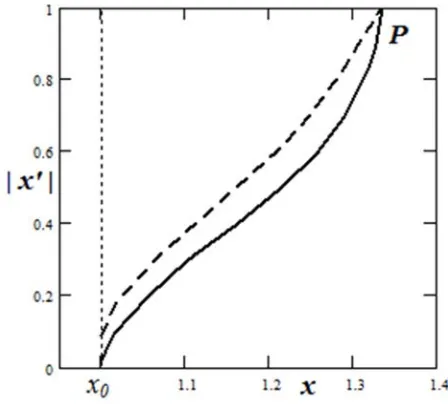
Figure 3 shows the phase portrait of the solution of equation (12). The qualitative behavior of the solution can be described as follows. In the moving system, the point representing the behavior of the particle begins to move along the branch, for which rs′ >0(dashed line in Figure 3), corresponding to an increase in the helix radius over time (Figure 1b). In the branch point P rs′ =1, what corresponds
( )
2rϕ′ → ∞ or dϕ →0, i.e. rotation is stopped. Then the point goes to another branch, for which rs′ <0 (solid line in the Figure 3) and, moving along this branch and rotating in the opposite direction, reaches the horizon r=r0 . More precisely, the motion of a point can be described on a two-dimensional surface embedded in a three-two-dimensional Euclidean space whose structure near the branch point resembles a torus. Point P corresponds to a transition from one side of the torus, on which the spiral is untwisting onto
the opposite side, where the spiral is twisting.
For the data in Figure 3, the horizonx0 =r0/rɶ=1.001. On
the horizon, the radial velocity of the point is
0
0 ( )
( )
dr r b
r ds
b r rϕ
δ ω
± =
− ′ɶ
(14)
The ± signs correspond to two branches of the solution, shown in Figure 3. Solving equation (14) with allowance for (13) we obtain the value r rs′( )0 ≈ ±δ ω/ in which the higher order terms with respect to the small parameter δ ω <</ 1 were omitted. Then, reaching the horizon, the point falls into a singularityr=0. This stage of the behavior of the point can not be described within the framework of the metric (8) and requires an additional investigation.
Figure 3. The phase portrait of the solution of equation (12);
0 2
/ , / ; 1.5
x=r rɶ>x x′=dr ds C = . The solid line and the dashed line show the two branches of the solution, dotted line – the horizon x ; 0 P−is the branch point. The calculations were performed for the first nontrivial zero of the ζ -function.
4. Metric in the Area Below the Horizon
As in the Schwarzschild case, the metric (8) is incomplete, because it is not applicable when r<r0[11]. Therefore, as well as solutions (10), it can be used only at distances exceeding r0.
To construct a metric suitable for r<r0, following [11], we perform the transformation of coordinates r t, →ρ τ, (omitting the strokes of t). Note, that a similar method was first applied by D. Finkelstein [11].
(
)
[
]
2
2 ,
1 ( ) 1 ( )
f d cd f d cd
dr cdt
f
A r B r
ρ τ ρ τ
⋅ ± ±
= =
−
where f(r) –is a function chosen from the condition that the fictitious singularity at r=r0of the metric (8) be eliminated. Performing the calculations, we find that this is achieved by choosing
[
]
1/ 2
2 2
1/ 2
( ) 1 ( ) r
f r A r
r δ ω = − = + ɶ (16)
The expression for the interval (8) in which we again introduce instead the variable l the angular variable φ, takes the form
( )
22 2 2 2 2
( )
ds = cd
τ
− f r dρ
−r dϕ
(17)The interval (17) has only the real singularity at the point r = 0. The metric (17) is synchronous (gττ =1) and is
nonstationary, as in the Schwarzschild case [11]. From (15) it follows the connection between the new and old coordinates
[
]
( ),
( ) 1 ( ) ( )
( )
c r
A r B r
r dr
f r
ρ τ± = Φ
−
Φ =
∫
(18)In variablesρ τ, , there is no singularity on the horizon 1
0 ( )
r= = Φr −
ρ τ
−c . The coordinate ρ is everywhere spatial, and τ− temporary. The given values of r are corresponded to the world linesρ τ−с =const. The world lines of a particle at rest relative to the reference frame described by coordinates ρ τ, are straight lines parallel to the axis τ. Moving along them, the particle enters the center of the field r=0 in a finite interval of proper time. As applied to our problem, this means that the series (1), divergent in a fixed coordinate system, converges in the moving system to the correct value ζ(s1)=0.Write out the system of equations of motion in the region below the horizon
2 2 2 2 2 2 2 2 2 0, 2 0, 1 0 d ds
d dr dr d
r d ds ds
ds
d df d r dr d
f d ds d ds
ds f
τ
ϕ ϕ
ρ
ρ ρ ϕ
ρ ρ = + = + − = (19)
where the expressions for the non-zero Christoffel symbols are used [11]. From the second equation of (19) we find the integral of system
[
]
( )
ln 2
( ) 1 ( )
d f r dr
const
ds r A r B r
ϕ± =
−
∫
(20)Taking into account that the integrand depends on dϕ/dr, the integral (20) allows in principle to find the solution of the
system (18) and calculate the time of the particle's fall into the singularity.
5. Consideration of the General Case
Let us apply our consideration to the general case when the argument of the ζ-function lies outside the critical line
Re 1 / 2
u= s= . We use to represent the partial sum (1) by the asymptotic Euler-Maclaurin formula [8] (one can find the proof in the textbooks on mathematics)
1
1 1
1
( ) , 1
1 , 0 1, 0
m m s s s m n m
s n n dn m
s
s u iv u v
ζ − − − +
=
−
= ≈ = >>
− = − < < >
∑
∫
(21)In the case m >> 1, one can neglect the unity in the numerator of the last expression. With the aid of (21) one can obtain asymptotically exact expressions for the quantities appearing in (2)
(
)
(
1)
1 1
arg m( ) arg m ( )
u m m m v s s m R e R
ζ ζ −
− +
− ≈
≈
(22)
and, hence, to obtain expressions for the components V Vr, ϕ of the velocity of the particle, which realizes the calculations
1
, ,
1
r
u v u
V V
u Crγ ϕ Crγ γ
−
= = =
− (23)
C is a constant. The case considered above corresponds 1/ 2
u= . For that case, we get the expressions used before
, 1 , 2 r V V r r v C C
ϕ
ω
δ
ω
δ
= =
= =
(24)
Hence we obtain a formula δ ω/ =1 / 2v, the validity of which with high precision is easily verified by means of Table 1.
It would be possible to develop the methodology described above with reference to the general case, but this is meaningless since the dependences of the velocities (23) do not correspond to the model of ideal liquid used to realize the relativistic computer proposed in this paper. To show this we use the so-called equation of dynamic motion possibility of A. A. Friedman [10] and which was used by Helmholtz for an incompressible fluid
( )
d
V divV dt
rotV
Ω = Ω⋅∇ −Ω Ω =
(25)
0
divV= . Writing it in cylindrical coordinates, we obtain condition
( )
111 2 1
0 1
u r
u
divV rV r
r u
− −
= = =
− (26)
which is valid only for u=1/ 2, i.e. on the critical line. A consequence of this is the possibility of giving the Riemann hypothesis the following formulation:
All the nontrivial zeros of the Riemann ζ-function are computable on a relativistic computer.
6. Discussions
The results of computing divergent series associated with the ζ-function can be clearly explained without using complicated calculations, using general physical considerations. Start with the result obtained in [1], devoted to the calculation of ζ (-1). In this case, we concentrate on the fact of obtaining a convergent series in a fixed system from the divergent series for ζ (-1) in the proper frame of reference, leaving aside getting specific value of the sum of the series - for this some calculations are needed, which are given in [1]. It was shown in [1] that as a moving system for calculating ζ (-1) one should take a system moving with respect to a rest system with constant acceleration, as long as the velocity of the moving system V << c (c is the speed of light). A naive (and solely right) way to represent the computation of a series for ζ (-1) is to sequentially attach segments on the real axis which length increases by 1 to the total segment corresponding to the next partial sum of the series
( 1) 1 2 3 ... n ...
ζ
− = + + + + + (27)where n -means the length of the n-th segment. This would look an attempt (unsuccessful) to calculate the sum of the series for ζ (-1) in a moving system relative to which the computational device is at rest. While observing the calculation of the initial series from the fixed system, with respect to which the computational device moves with acceleration, we obtain another scheme
(
)
1 2 2
2
( 1) 1 2 3 ... ...
1 /
n
n n
n
V c
ζ β β β β
β
− = + + + + +
= − (28)
where βn– is a Lorentz factor, and Vn– is the velocity of the
moving system at the moment of adding the n-th term of the series. Due to this, the series representing ζ (-1) converges and has a finite sum.
To explain the computation of the ζ-function of the complex argument, performed in the present paper, write the last equation (10) in the form
2 4
2 1
( ) ,
2 2 ( )
r
b A
d dr
B r y y
dr A r ds
′
= =
(29)
which represents the law of conservation of energy for a particle having velocity rs′ and mass B r( ). Integrating (29) with respect to r in the range from r1 to r2>r1>r0, we obtain
that the change in the kinetic energy By/ 2of the particle on the virtual displacement from r1 to r2 is equal to the work of
the force b A4 ′/ 2A2 on this displacement, which, as seen from expression (8), is positive. This means that the force is directed to the growth of r. However, the acceleration of the particle is directed in the opposite direction due to the negativity of the mass B for r > r0. This leads eventually to
the convergence of the series (1) in the moving system.
7. Conclusion
In this article the computation of the Riemann ζ-function represented by a divergent series in the plane of the complex argument is performed using the methods of the general theory of relativity. The calculation is realized by the motion of some material particle in a curved metric. It is shown that the non-computable (in the sense of Turing) problem of computation of the sum of a divergent series becomes computable in the transition to the moving system of reference. In this sense, the result of the work confirms the perspective of the direction associated with the so-called relativistic supercomputers [3], which received the conventional name "Beyond Turing". The difference of this work from the majority of works of the mentioned direction is the absence of the need to involve cosmological black holes for the realization of calculations. The curvature of the metric necessary for this purpose arises as a result of the motion of the computational particle (ensemble of particles), in accordance with the equations of hydrodynamics of an ideal fluid, which creates the corresponding singular metric. In fact, it is the implementation of the thesis, inverse to the well-known thesis on the computational nature of motions in the Universe [4].
The character of the mobile frame of reference and its metric has been determined; the equations of motion of a material particle in this metric are solved. The resulting metric, like the Schwarzschild metric, has a fictitious singularity separating the inner region under the horizon from the outer one. This metric can be extended to the inner area, which eliminates the fictitious singularity. The motion in the inner region looks like the drop of the particle to the center in a finite proper time, which proves the convergence of the series under consideration, i.e., solution of an initially incomputable problem.
The results concerning the properties of non-trivial zeros of ζ-functions, taking into account their connection with the distribution of primes, are of great importance in solving information security issues [13].
References
[2] G. H. Hardy, Divergent series, Oxford, 1949.
[3] I. Nemeti, G. David, Relativistic computers and the Turing barrier. Applied Mathematics and Computation, 178, 118-142, 2006.
[4] S. Lloyd, Programming the Universe. A Quantum Computer Scientist Takes on the Cosmos, Knopf, 2006.
[5] W. J. Cody, K. E. Hillstrom, Thacher, C. Henry, Jr, Chebyshev approximations for the Riemann zeta function. Math. Comp. -1971.-№25. С. 537–547.
[6] R. L. Graham, D. E. Knuth, O. Patashnick, Concrete Mathematics. A Foundation for Computer Science, 2nd Ed, Addison-Wesley, 1994.
[7] E. A. Karatsuba, Rapid computation of the Riemann zeta-function ζ (s) for integer values of the argument s, Problems of information transfer. -1995. -№31.-P. 69-80. (Russian).
[8] A. A. Karatsuba, Foundations of Analytic Number Theory. – Moscow, Science, 1983. (Russian).
[9] E. Janke, F. Emde, F. Lösch, Tafeln Höherer Funktionen, B. G. Teubner Verlagsgeselschaft, Stuttgart, 1960.
[10] L. G. Loitsyansky, Mechanics of Liquids and Gases, Moscow, Leningrad, GITTL, 1950 (Russian).
[11] L. D. Landau, E. M. Lifshitz, The Classical Theory of Fields, (4th ed.), Butterworth-Heinemann, 1975.
[12] R. C. Tolman, Relativity Thermodynamics and Cosmology, Clarendon Press, Oxford, 1969.
![Figure 1. Calculation results of ζm(s1); s1=0.5-14.134725i - first non-trivial zero of ζ-function [9]](https://thumb-us.123doks.com/thumbv2/123dok_us/9900453.1977487/2.595.114.482.470.657/figure-calculation-results-zm-non-trivial-zero-function.webp)